Many-Body Density Matrices On a Two-Dimensional Square Lattice:
Noninteracting and Strongly Interacting Spinless Fermions

Abstract

The reduced density matrix of an interacting system can be used as the basis for a truncation scheme, or in an unbiased method to discover the strongest kind of correlation in the ground state. In this paper, we investigate the structure of the many-body fermion density matrix of a small cluster in a square lattice. The cluster density matrix is evaluated numerically over a set of finite systems, subject to non-square periodic boundary conditions given by the lattice vectors $\mathbf{R}_{1}\equiv(R_{1x},R_{1y})$ and $\mathbf{R}_{2}\equiv(R_{2x},R_{2y})$. We then approximate the infinite-system cluster density-matrix spectrum, by averaging the finite-system cluster density matrix (i) over degeneracies in the ground state, and orientations of the system relative to the cluster, to ensure it has the proper point-group symmetry; and (ii) over various twist boundary conditions to reduce finite size effects. We then compare the eigenvalue structure of the averaged cluster density matrix for noninteracting and strongly-interacting spinless fermions, as a function of the filling fraction $\bar{n}$, and discuss whether it can be approximated as being built up from a truncated set of single-particle operators.

I Introduction

The density matrix is a very useful tool in the numerical study of interacting systems. Besides being used in the Density-Matrix Renormalization Group (DMRG)white92 and its higher-dimensional generalizations,verstraete04 the density matrix is also used as a diagnostic tool in the Contractor Renormalization (CORE) method for numerical renormalization group in two dimensions,core and forms the basis of a method to identify the order parameter related to a quasi-degeneracy of ground states.furukawa05

In previous work,cheong04a we extended the results of Chung and Peschelchung01 to write the density matrix (DM) of a cluster of $N_{C}$ sites cut out from a system of noninteracting spinless fermions in $d$ dimensions as the exponential of a quadratic operator, called the pseudo-Hamiltonian, as it resembles the Hamiltonian of a noninteracting system. That result was then applied in numerical studies of noninteracting spinless fermions in one dimension, to better understand how the distribution of cluster DM eigenvalues scale with $N_{C}$, and to explore the possibility of designing truncation schemes based on the pseudo-Hamiltonian.cheong04b We believe truncation schemes such as that described in Ref. cheong04b, will be helpful to the choice of basis states in renormalization groups such as CORE.

Thus, some questions motivating the present paper were: (i) does the density matrix of an interacting Fermi-liquid system resembles that of a noninteracting one? (ii) can we apply our exact result in Ref. cheong04a, to two dimensions as well as for one dimension? (iii) is it numerically practical to compute this sort of density matrix in a fermion system. To answer these questions, we investigated a spinless analog of the extended Hubbard model, given by the Hamiltonian

$$H=-t\sum_{\braket{i,j}}{c_{i}^{\dagger}}{c_{j}^{\phantom{\dagger}}}+V\sum_{\braket{i,j}}n_{i}n_{j},$$ (1)

in the limit of $V\to\infty$, so that fermions are not allowed to be nearest neighbors of each other. This model is chosen for two reasons: (i) for a given number of particles, the $V\to\infty$ Hilbert space is significantly smaller than the $V<\infty$ Hilbert space, and we can work numerically with larger system sizes; and (ii) the model, in spite of its simplicity, has a rich zero-temperature phase diagram,zhang01 ; zhang03 ; zhang04 where we find practically free fermions in the limit $\bar{n}\ll 1$, and an inert solid at half-filling $\bar{n}=\frac{1}{2}$. As the filling fraction approaches quarter-filling from below, $\bar{n}\to\frac{1}{4}^{-}$, the system becomes congested, highly correlated, but is nonetheless a Fermi liquid, perhaps with additional orders that are not clear in small systems. Slightly above quarter-filling, the dense fluid and inert solid coexists, while slightly below half-filling, the system is expected to support stable arrays of stripes.

To probe this rich variety of structures in the ground state at different filling fraction $\bar{n}$, we describe in Section II how the reduced DM of a small cluster, with the appropriate symmetry properties, can be calculated from a finite non-square system subject to twist boundary conditions. Then in Section III, we investigate in great details the cluster DM spectra of the noninteracting system, particularly on how to handle finite size effects in the numerics, for comparison with the cluster DM spectra of a strongly-interacting system, presented in Section IV. Finally, in Section V, we summarized our findings, and discuss the prospects of designing an Operator-Based DM Truncation Scheme for interacting systems, at some, if not at all, filling fractions.

II Formulation

In this section, we give the theoretical formulations and describe the numerical tools needed to investigate the cluster DM spectra of noninteracting and strongly-interacting systems of spinless fermions in two dimensions. In Section II.1, we give the matrix elements of the DM of a small cluster embedded within a larger, but still finite, system. These matrix elements are obtained by tracing out degrees of freedom external to the cluster, starting from the ground-state wave function of the system, obtained through exact diagonalization. In Section II.2, we describe how our finite systems can be defined with nonsquare periodic boundary conditions, and how we make use of the translational invariance of both noninteracting and strongly-interacting models to reduce the computational efforts in exact diagonalization. In Section II.3, we describe several averaging apparatus required to obtain a handle on the infinite-system spectra of the cluster DM, and then in Section II.4, we describe a classification scheme for the one-particle and multi-particle eigenstates of the cluster DM that makes the symmetry of the underlying square lattice explicit.

II.1 Cluster Density Matrix

The DM $\rho_{C}$ of a cluster cut out from a larger system is a density operator which gives the expectation

$$\braket{\Psi}{A}{\Psi}=\braket{A}=\operatorname{Tr}_{C}\rho_{C}A$$ (2)

for any observable $A$ local to the cluster, when the larger system is in its ground state $\ket{\Psi}$. The cluster DM $\rho_{C}$ can be calculated from the ground-state DM

$$\rho=\ket{\Psi}\bra{\Psi}$$ (3)

of the system, by tracing out degrees of freedom outside of the cluster. We write this as

$$\rho_{C}=\operatorname{Tr}_{E}\rho,$$ (4)

where the subscript $E$ denotes a trace over environmental degrees of freedom.

Since a cluster is a collection of sites identified in real space, it is natural to choose as a many-body basis the real-space configurations. For a finite two-dimensional system with $N$ sites, we label the sites $j=1$ through $j=N$, so that for any pair of sites $(x_{j_{1}},y_{j_{1}})$ and $(x_{j_{2}},y_{j_{2}})$, we have $x_{j_{1}}\leq x_{j_{2}}$ and $y_{j_{1}}<y_{j_{2}}$ if $j_{1}<j_{2}$. We then distinguish between sites within the cluster, of which there are $N_{C}$ of them, $(x_{j_{1}^{C}},y_{j_{1}^{C}})$, $(x_{j_{2}^{C}},y_{j_{2}^{C}})$, …, $(x_{j_{N_{C}}^{C}},y_{j_{N_{C}}^{C}})$, and sites outside of the cluster, of which there are $N_{E}=N-N_{C}$ of them, $(x_{j_{1}^{E}},y_{j_{1}^{E}})$, $(x_{j_{2}^{E}},y_{j_{2}^{E}})$, …, $(x_{j_{N_{E}}^{E}},y_{j_{N_{E}}^{E}})$. We think of the $N_{E}$ sites outside the cluster as constituting the environment to the cluster.

We work with the configuration basis states $\ket{\mathbf{j}}=\ket{j_{1}j_{2}\cdots j_{P}}$, where $j_{1}<\cdots<j_{P}$ are the $P$ occupied sites in the system. These can be thought of as a direct product of the configuration basis states of the cluster $\ket{\mathbf{l}}=\ket{l_{1}l_{2}\cdots l_{P_{C}}}$, where $l_{1}<\cdots<l_{P_{C}}$ are the $P_{C}$ occupied sites within the cluster, and the configuration basis states of the environment $\ket{\bm{missing}}=\ket{m_{1}m_{2}\cdots m_{P_{E}}}$, where $m_{1}<\cdots<m_{P_{E}}$ are the $P_{E}=P-P_{C}$ occupied sites in the environment. Here, we have the occupied sites of the system $\{j_{1},\dots,j_{P}\}=\{l_{1},\dots,l_{P_{C}}\}\cup\{m_{1},\dots,m_{P_{E}}\}$ being the union of the occupied sites in the cluster and in the environment, with the site indices $l$ and $m$ resorted in ascending order to give the site indices $j$.

In terms of the configuration basis of the system, the ground-state wave function of the system can be written as

$$\ket{\Psi}=\sum_{\mathbf{j}}\Psi_{\mathbf{j}}\ket{\mathbf{j}}=\sum_{\mathbf{j}}\Psi_{\mathbf{j}}{c_{j_{1}}^{\dagger}}\cdots{c_{j_{P}}^{\dagger}}\ket{0},$$ (5)

where $\Psi_{\mathbf{j}}$ is the amplitude associated with configuration $\ket{\mathbf{j}}$, and ${c_{j}^{\phantom{\dagger}}}$, ${c_{j}^{\dagger}}$ are fermion annihilation and creation operators acting on the site $(x_{j},y_{j})$. We can also write the ground-state wave function as

$$\begin{split}\ket{\Psi}&=\sum_{\mathbf{l}}\sum_{\bm{}}(-1)^{f(\mathbf{j};\mathbf{l},\bm{)}}\Psi_{\mathbf{l},\bm{}}\ket{\mathbf{l}}\ket{\bm{missing}}\\ &=\sum_{\mathbf{l}}\sum_{\bm{}}(-1)^{f(\mathbf{j};\mathbf{l},\bm{)}}\Psi_{\mathbf{l},\bm{}}\times{}\\ &\qquad\qquad\qquad{c_{m_{1}}^{\dagger}}\cdots{c_{m_{P_{E}}}^{\dagger}}{c_{l_{1}}^{\dagger}}\cdots{c_{l_{P_{C}}}^{\dagger}}\ket{0},\end{split}$$ (6)

in terms of the direct product of configuration bases of the cluster and the environment, where ${c_{l}^{\phantom{\dagger}}}$ and ${c_{l}^{\dagger}}$ are fermion annihilation and creation operators acting on site $(x_{l},y_{l})$ within the cluster, and ${c_{m}^{\phantom{\dagger}}}$ and ${c_{m}^{\dagger}}$ are fermion annihilation and creation operators acting on site $(x_{m},y_{m})$ within the environment. In (6), the amplitude $\Psi_{\mathbf{l},\bm{}}=\Psi_{\mathbf{j}}$ is taken directly from the expansion in (5), while the factor $(-1)^{f(\mathbf{j};\mathbf{l},\bm{)}}$ accounts for the fermion sign incurred when we reorder the operator product ${c_{m_{1}}^{\dagger}}\cdots{c_{m_{P_{E}}}^{\dagger}}{c_{l_{1}}^{\dagger}}\cdots{c_{l_{P_{C}}}^{\dagger}}$ to get the operator product ${c_{j_{1}}^{\dagger}}\cdots{c_{j_{P}}^{\dagger}}$.

Similarly, the ground-state DM in (3) can be written as

$$\rho=\sum_{\mathbf{j}}\sum_{\mathbf{j}^{\prime}}\Psi_{\mathbf{j}}\Psi_{\mathbf{j}^{\prime}}^{*}{c_{j_{1}}^{\dagger}}\cdots{c_{j_{P}}^{\dagger}}\ket{0}\bra{0}{c_{j^{\prime}_{P}}^{\phantom{\dagger}}}\cdots{c_{j^{\prime}_{1}}^{\phantom{\dagger}}},$$ (7)

using the system-wide configuration basis, or as

$$\rho=\sum_{\mathbf{l},\bm{}}\sum_{\mathbf{l}^{\prime},\bm{{}^{\prime}}}(-1)^{f(\mathbf{j};\mathbf{l},\bm{)}+f(\mathbf{j}^{\prime};\mathbf{l}^{\prime},\bm{{}^{\prime}})}\Psi_{\mathbf{l},\bm{}}\Psi_{\mathbf{l}^{\prime},\bm{{}^{\prime}}}^{*}\times{}\\ {c_{m_{1}}^{\dagger}}\cdots{c_{m_{P_{E}}}^{\dagger}}{c_{l_{1}}^{\dagger}}\cdots{c_{l_{P_{C}}}^{\dagger}}\ket{0}\times{}\\ \bra{0}{c_{l^{\prime}_{P^{\prime}_{C}}}^{\phantom{\dagger}}}\cdots{c_{l^{\prime}_{1}}^{\phantom{\dagger}}}{c_{m^{\prime}_{P^{\prime}_{E}}}^{\phantom{\dagger}}}\cdots{c_{m^{\prime}_{1}}^{\phantom{\dagger}}},$$ (8)

using the direct-product basis between cluster configurations and environment configurations.

Performing the trace over the environment as prescribed in (4), we find the fermion cluster DM $\rho_{C}$ to be

$$\rho_{C}=\sum_{\mathbf{l},\mathbf{l}^{\prime}}\sum_{\bm{,}\bm{{}^{\prime}}}(-1)^{f(\mathbf{j};\mathbf{l},\bm{)}+f(\mathbf{j}^{\prime};\mathbf{l}^{\prime},\bm{{}^{\prime}})}\times{}\\ \Psi_{\mathbf{l},\bm{}}\Psi_{\mathbf{l}^{\prime},\bm{{}^{\prime}}}^{*}\delta_{\bm{,}\bm{{}^{\prime}}}\times{}\\ {c_{l_{1}}^{\dagger}}\cdots{c_{l_{P_{C}}}^{\dagger}}\ket{0}\bra{0}{c_{l^{\prime}_{P^{\prime}_{C}}}^{\phantom{\dagger}}}\cdots{c_{l^{\prime}_{1}}^{\phantom{\dagger}}}.$$ (9)

Its matrix elements are

$$\braket{\mathbf{l}}{\rho_{C}}{\mathbf{l}^{\prime}}=\sum_{\bm{}}\sum_{\bm{{}^{\prime}}}(-1)^{f(\mathbf{j};\mathbf{l},\bm{)}+f(\mathbf{j}^{\prime};\mathbf{l}^{\prime},\bm{{}^{\prime}})}\times{}\\ \Psi_{\mathbf{l},\bm{}}\Psi_{\mathbf{l}^{\prime},\bm{{}^{\prime}}}^{*}\delta_{\bm{,}\bm{{}^{\prime}}}.$$ (10)

These matrix elements can be computed naively by running over all possible pairs of cluster states $\ket{\mathbf{l}}$ and $\ket{\mathbf{l}^{\prime}}$, and performing the sums over $\bm{$}and$’$astheyappearin\eqref{eqn:detailrhocmatrixelements},lookingupthefermion-signfactors$(-1)^f(j;l,)$andamplitudes$Ψ_l,$asandwhentheyareneeded.Wecallthisthe\emph{naive algorithm}.Alternatively,wecanalsoreorganizethefermion-sign-factor-adjustedamplitudes$(-1)^f(j;l,)Ψ_l,$intoamatrix$~Ψ$,whoserowsareassociatedwiththeclusterconfigurations$—l⟩$,andwhosecolumnsareassociatedwiththeenvironmentconfigurations$—missing⟩$,thematrix$ρ_C$canbecomputeddirectlybymatrixmultiplicationas\begin{equation}\rho_{C}=\tilde{\boldsymbol{\Psi}}\tilde{\boldsymbol{\Psi}}^{\dagger},\end{equation}representingacollectionofinnerproducts.Wecallthisthe\emph{pre-sorted inner-product algorithm}.WecompareandanalyzethecomputationalcomplexityofthesetwoalgorithmsinAppendix\ref{appendix:computational}.InthenumericalstudiespresentedinSection\ref{sect:strong},weusethepre-sortedinner-productalgorithmexclusively.\par From\eqref{eqn:presortinnerproduct},weseethattheclusterDM$ρ_C$ismanifestlyhermitian,andthusallitseigenvalues${w}$arereal(andinfactnonnegative).Whenobtainedfromthewavefunctionofastatewithdefiniteparticlenumber,$ρ_C$hasnomatrixelementsbetweenclusterstatescontainingdifferentnumberofparticles,andthustheeigenstates$—w⟩$of$ρ_C$canbeorganizedinto\emph{sectors},correspondingto$P_C = 0, 1, …, P_C,max$particleswithinthecluster.Fortherestofthispaper,wewouldrefertotheeigenvaluesof$ρ_C$genericallyasits\emph{weights},sincethesehaveanaturalprobabilisticinterpretation.A$P_C$-particleweightof$ρ_C$isthereforeaneigenvaluecorrespondingtoaneigenstatecontaining$P_C$particleswithinthecluster.\par$

II.2 System Definition and Translational Invariance

For noninteracting spinless fermions on an infinite square lattice, it is possible to compute the cluster DM $\rho_{C}$ starting from the Fermi sea ground state, through the evaluation and diagonalization of $G_{C}$. For an interacting system, we need to compute $\rho_{C}$ starting from $\rho$ in (3), the latter we obtain through exact diagonalization on a finite system. We define the a finite system relative to the infinite square lattice in terms of the lattice vectors $\mathbf{R}_{1}$ and $\mathbf{R}_{2}$, as shown in Fig. 1, such that $N=\hat{\mathbf{z}}\cdot(\mathbf{R}_{1}\times\mathbf{R}_{2})=R_{1x}R_{2y}-R_{2x}R_{1y}>0$ is the number of lattice sites within the system.

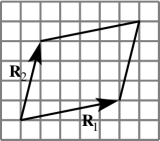
Figure 1: Definition of system to be exactly diagonalized in terms of the lattice vectors $\mathbf{R}_{1}$ and $\mathbf{R}_{2}$. We shall denote such a system as $\mathbf{R}_{1}\times\mathbf{R}_{2}$. In this example shown, the system is $(5,1)\times(1,4)$.

If we impose periodic boundary condition such that $\mathbf{R}+m\mathbf{R}_{1}+n\mathbf{R}_{2}\equiv\mathbf{R}$, then in the exact diagonalization to obtain $\ket{\Psi}$ we can take advantage of translational invariance through the use of the Bloch states

$$\ket{\mathbf{j}_{0},\mathbf{k}}=\frac{1}{\sqrt{N}}\sum_{\mathbf{R}}e^{-\mathrm{i}\mathbf{k}\cdot\mathbf{R}}T_{\mathbf{R}}\ket{\mathbf{j}_{0}}$$ (12)

as our computational basiszhang03 . In this Bloch state, the configurations $\{T_{\mathbf{R}}\ket{\mathbf{j}_{0}}\}$ are all related to the generating configuration $\ket{\mathbf{j}_{0}}$ by the lattice translations $T_{\mathbf{R}}$ associated with displacement $\mathbf{R}$, while $\mathbf{k}$ are wave vectors allowed by the boundary conditions. Any configuration within the collection of translationally-related configurations $\{T_{\mathbf{R}}\ket{\mathbf{j}_{0}}\}$ can serve as the generating configuration, but we pick the one with the least sum of indices of occupied sites.

Working with finite non-square systems introduces several complications. First of all, we sometimes end up with degenerate ground states which suffer from symmetry-breaking not found in the true infinite-system ground state. However, because the point symmetry group of our non-square finite system is only a subgroup of the square lattice point symmetry group, the finite-system ground-state manifold is not invariant under all square lattice symmetry operations. Thirdly, when working with finite systems, we introduce systematic deviations which are collectively known as finite size effects. We identify the three primary sources of finite size effects as (i) finite domain effect, which has to do with the fact that the small set of discrete wave vectors allowed are not adequately representative of the continuous set of wave vectors on the infinite square lattice; (ii) shell effect, which has to do with the fact that the set of discrete wave vectors allowed are organized by symmetry into shells in reciprocal space, each of which can be partially or fully filled in the many-body ground state; and (iii) shape effect, which has to do with the detailed shape of the non-square system we introduced.

II.3 Averaging

II.3.1 Degeneracy Averaging

To eliminate these numerical artefacts, we adopted three averaging devices. First, we average over the $D_{0}$-fold degenerate ground-state manifold. Our first motivation for doing so is as follows: if $\mathscr{G}$ is the point symmetry group of the square lattice, and its subgroup $G$ is the point symmetry group of the $\mathbf{R}_{1}\times\mathbf{R}_{2}$ system, then we will find that the cluster density matrices

$$\rho_{C,i}=\operatorname{Tr}_{E}\ket{\Psi_{i}}\bra{\Psi_{i}},$$ (13)

one for each wave function $\Psi_{i}$ within the $D_{0}$-fold degenerate ground-state manifold, are not invariant under $G$, much less $\mathscr{G}$. We remove this artificial symmetry breaking by calculating the degeneracy-averaged cluster DM

$$\rho_{C}=\frac{1}{D_{0}}\sum_{i=1}^{D_{0}}\rho_{C,i}$$ (14)

over the cluster density matrices $\rho_{C,i}$ within the ground-state manifold. This degeneracy-averaged cluster DM is invariant under $G$.

A second motivation for such a mode of averaging over the degenerate ground-state manifold of the finite system is that thermodynamically, given the pure state density matrices $\rho_{C,i}$, with energy eigenvalue $E_{i}$, we typically construct the canonical ensemble DM as

$$\rho_{C}(\beta)=Z^{-1}(\beta)\sum_{i}e^{-\beta E_{i}}\,\rho_{C,i},$$ (15)

where $Z(\beta)=\sum_{i}e^{-\beta E_{i}}$ is the canonical partition function. States within a degenerate manifold have the same energy, and therefore contribute equally to the thermodynamic DM $\rho_{C}(\beta)$. In the limit of $\beta\to\infty$, the usual thermodynamic argument is that pure states decouple from one another, and we treat their respective density matrices independently, except for those states which are degenerate. Because they appear with the same Boltzmann weight whatever the inverse temperature is, we should still treat the uniform combination instead of the individual density matrices in the limit of $\beta\to\infty$,

II.3.2 Orientation Averaging

The second averaging device involves an average over the orientation of the finite non-square system relative to the underlying square lattice. This averaging restores the $\mathscr{G}$-symmetry to the averaged ground state. In principle, this requires us to compute $\rho_{C}$ for a group of four systems: $(R_{1x},R_{1y})\times(R_{2x},R_{2y})$, $(R_{2y},R_{2x})\times(R_{1y},R_{1x})$, $(R_{1x},-R_{1y})\times(-R_{2x},R_{2y})$ and $(R_{2y},-R_{2x})\times(-R_{1y},R_{1x})$.

However, if the cluster whose DM we are calculating is invariant under the action of $\mathscr{G}$, this averaging can be achieved by computing

$$\bar{\rho}_{C}=\frac{1}{D(\mathscr{G})}\sum_{g\in\mathscr{G}}U_{g}\rho_{C}U_{g}^{\dagger},$$ (16)

where $g\in G$ is a point group transformation of the square lattice, $U_{g}$ is the unitary transformation of the cluster Hilbert space associated with $g$, and $D(\mathscr{G})$ is the order of $\mathscr{G}$.

II.3.3 Twist Boundary Conditions Averaging

After these two averagings, the cluster DM has the full symmetry (including translations) of the underlying square lattice, but finite size effects remain. We eliminate these as much as we cancheong05 with the third averaging device, twist boundary conditions averaging.twist The usual way to implement twist boundary conditions is to work in the boundary gauge, keeping the Hamiltonian unchanged, and demanding that

$${c_{\mathbf{R}+\mathbf{R}_{1}}^{\phantom{\dagger}}}=e^{-\mathrm{i}\boldsymbol{\phi}\cdot\mathbf{R}_{1}}\,{c_{\mathbf{R}}^{\phantom{\dagger}}},\quad{c_{\mathbf{R}+\mathbf{R}_{2}}^{\phantom{\dagger}}}=e^{-\mathrm{i}\boldsymbol{\phi}\cdot\mathbf{R}_{2}}\,{c_{\mathbf{R}}^{\phantom{\dagger}}},$$ (17)

where $\mathbf{R}_{1}$ and $\mathbf{R}_{2}$ are the lattice vectors defining our finite system, $\mathbf{R}=(R_{x},R_{y})$ is a site within the system, and $\boldsymbol{\phi}=(\phi_{x},\phi_{y})$ is the twist vector parametrizing the twist boundary conditions.

In choice of gauge (17), the Hamiltonian (1) is not manifestly invariant under translations. However, we can continue to block-diagonalize it using the Bloch basis states defined in (12), provided the set of allowed wave vectors $\mathbf{k}$ are shifted relative to $\mathbf{k}_{0}$ for the usual periodic boundary conditions by the twist vector $\boldsymbol{\phi}$, i.e.

$$\mathbf{k}=\mathbf{k}_{0}+\boldsymbol{\phi}.$$ (18)

The other natural way to implement twist boundary conditions is in the bond gauge, where we make the substitution

$${c_{\mathbf{R}}^{\phantom{\dagger}}}\to e^{-\mathrm{i}\mathbf{R}\cdot\boldsymbol{\phi}}{c_{\mathbf{R}}^{\phantom{\dagger}}}$$ (19)

in the Hamiltonian, but demand that

$${c_{\mathbf{R}+\mathbf{R}_{1}}^{\phantom{\dagger}}}={c_{\mathbf{R}}^{\phantom{\dagger}}},\quad{c_{\mathbf{R}+\mathbf{R}_{2}}^{\phantom{\dagger}}}={c_{\mathbf{R}}^{\phantom{\dagger}}},$$ (20)

where $\mathbf{R}_{1}$ and $\mathbf{R}_{2}$ are the lattice vectors defining our finite system. Now the Hamiltonian (1) is manifestly invariant under translations, and we can bloch-diagonalize it using the Bloch basis states defined in (12), with the same set of allowed wave vectors $\mathbf{k}=\mathbf{k}_{0}$ as for the usual periodic boundary conditions.

Exact diagonalization can be performed in any gauge, but we chose to do it in the bond gauge, because in this gauge, the Bloch basis states $\ket{\mathbf{j}_{0},\mathbf{k}}$ defined in (12) can be used as is to block diagonalize the Hamiltonian at all twist vectors $\boldsymbol{\phi}$. This gives us the ground-state wave function $\ket{\Psi(\text{bond})}$ in the bond gauge. In the boundary gauge, or any other gauges, appropriate gauge transformations must be applied to $\ket{\mathbf{j}_{0},\mathbf{k}}$ before we can use this Bloch basis to block diagonalize the Hamiltonian. Because of this, the computational cost for exact diagonalization incurred in the bond gauge is fractionally lower than in other gauges.

We can also calculate the correlation functions $\braket{\tilde{O}(\mathbf{R})\tilde{O}^{\prime}(\mathbf{R}+\Delta\mathbf{R})}$ (of which the cluster DM is a function of) in any gauge, with appropriately-defined covariant observables $\tilde{O}=UOU^{\dagger}$, where $O$ are the ‘physical’ observables we would use when there is no twist in the boundary conditions. In the boundary gauge, these covariant observables $\tilde{O}=O$ and $\tilde{O}^{\prime}=O^{\prime}$ are particularly simple, except when the displacement vector $\Delta\mathbf{R}$ crosses the boundaries of our system. For our purpose of calculating the cluster DM, this situation occurs only when the cluster itself straddle the system boundaries. Therefore, with the cluster properly nested within the system, we chose to perform twist boundary conditions averaging in the boundary gauge.

In the boundary gauge, the cluster DM is obtained by tracing down the ground-state wave function $\ket{\Psi(\text{boundary})}$. We can get this wave function from $\ket{\Psi(\text{bond})}$ by applying the gauge transformation

$$\varphi:\ket{\mathbf{n}}\to e^{-i\sum_{\mathbf{R}}n_{\mathbf{R}}\mathbf{R}\cdot\boldsymbol{\phi}}\ket{\mathbf{n}},$$ (21)

where $\ket{\mathbf{n}}$ is an occupation number basis state, with occupation $n_{\mathbf{R}}$ on site $\mathbf{R}$.

Now, averaging over twist vectors $\boldsymbol{\phi}$ is the same as integrating over the Brillouin Zone, so we perform twist boundary conditions averaging over a uniform grid of Monkhorst-Pack points with order $q$.monkhorst76 For rectangular systems $(L_{x},0)\times(0,L_{y})$, the First Brillouin Zone is sampled by varying the two independent twist angles between $-\pi/L_{x}\leq\phi_{x}<+\pi/L_{x}$ and $-\pi/L_{y}\leq\phi_{y}<+\pi/L_{y}$. For non-square systems, the two independent twist angles $\phi_{1}$ and $\phi_{2}$ are defined by

$$e^{i\boldsymbol{\phi}\cdot\mathbf{R}_{1}}=e^{i\phi_{1}},\quad e^{i\boldsymbol{\phi}\cdot\mathbf{R}_{2}}=e^{i\phi_{2}}.$$ (22)

The twist vector $\boldsymbol{\phi}$ is then related to the independent twist angles $-\pi\leq\phi_{1}<+\pi$ and $-\pi\leq\phi_{2}<+\pi$ by

$$\boldsymbol{\phi}=\frac{\phi_{1}}{2\pi}\,\mathbf{Q}_{1}+\frac{\phi_{2}}{2\pi}\,\mathbf{Q}_{2},$$ (23)

where

$$\mathbf{Q}_{1}=\frac{2\pi}{N}(R_{2y},-R_{2x}),\quad\mathbf{Q}_{2}=\frac{2\pi}{N}(-R_{1y},R_{1x})$$ (24)

are the primitive reciprocal lattice vectors of our non-square system. For such systems, the First Brillouin Zone is a parallelogram on the $\phi_{x}$-$\phi_{y}$ plane, so the uniform grid of Monkhorst-Pack points are imposed on the square domain $(-\pi,+\pi)\times(-\pi,+\pi)$ on the $\phi_{1}$-$\phi_{2}$ plane instead.

II.4 Classifying States of the Cluster

The point symmetry group of the square lattice is the dihedral group $D_{4}$, which has eight elements.dihedral The five irreducible representations of this group are $A_{1}$, $A_{2}$, $B_{1}$, $B_{2}$ and $E$. For the cross-shaped cluster shown in Fig. 2, there is a one-to-one correspondence between these five irreducible representations and the one-particle states, but instead of labeling these one-particle states as $\ket{A_{1}}$, $\ket{A_{2}}$, $\ket{B_{1}}$, $\ket{B_{2}}$ and $\ket{E}$, we adopt an angular momentum-like notation,

$$\ket{s_{+}} =\ket{A_{1}}=\tfrac{1}{\sqrt{5}}(1,1,1,1,1),$$ (25)

$$\ket{s_{-}} =\ket{A_{2}}=\tfrac{1}{\sqrt{5}}(1,1,-1,1,1),$$

$$\ket{p_{x}} =\ket{B_{1}}=\tfrac{1}{\sqrt{2}}(1,0,0,0,-1),$$

$$\ket{p_{y}} =\ket{B_{2}}=\tfrac{1}{\sqrt{2}}(0,1,0,-1,0),$$

$$\ket{d} =\ket{E}=\tfrac{1}{2}(1,-1,0,-1,1).$$

that would make clear the structure of these one-particle states. We find it more convenient to work with the one-particle states

$$\ket{s} =\tfrac{1}{\sqrt{2}}\ket{s_{+}}+\tfrac{1}{\sqrt{2}}\ket{s_{-}}=\tfrac{1}{2}(1,1,0,1,1),$$ (26)

$$\ket{\bar{s}} =(0,0,1,0,0),$$

$$\ket{p_{+}} =\tfrac{1}{\sqrt{2}}\ket{p_{x}}+\tfrac{i}{\sqrt{2}}\ket{p_{y}}=\tfrac{1}{2}(1,i,0,-i,-1),$$

$$\ket{p_{-}} =\tfrac{1}{\sqrt{2}}\ket{p_{x}}-\tfrac{i}{\sqrt{2}}\ket{p_{y}}=\tfrac{1}{2}(1,-i,0,i,-1).$$

Figure 2: The five-site, cross-shaped cluster whose cluster DM we are interested in calculating for both a system of noninteracting, as well as strongly-interacting spinless fermions.

For a cluster DM possessing the full point group symmetry of the square lattice, the one-particle state $\ket{d}$ is constrained by symmetry to always be an eigenstate of $\rho_{C}$. We call the associated eigenvalue $w_{d}$ the weight of $\ket{d}$. Furthermore, the one-particle states $\ket{p_{x}}$ and $\ket{p_{y}}$ are also equivalent under the square lattice symmetry, and hence their weights $w_{p_{x}}$ and $w_{p_{y}}$ are equal. We call this doubly-degenerate one-particle weight $w_{p}$. On the other hand, the $s$ one-particle eigenstates of $\rho_{C}$ are in general not $\ket{s_{+}}$, $\ket{s_{-}}$ or $\ket{s}$, $\ket{\bar{s}}$, but some admixture of the form

$$\ket{s_{1}} =\cos\theta\ket{s}+\sin\theta\ket{\bar{s}},$$ (27)

$$\ket{s_{2}} =-\sin\theta\ket{s}+\cos\theta\ket{\bar{s}}.$$

We call their corresponding weights $w_{s_{1}}$ and $w_{s_{2}}$ respectively.

We can then extend this angular-momentum-like notation to multi-particle states of the cluster. Though the quantum numbers used to label the one-particle states are, strictly speaking, not angular momentum quantum numbers, we apply the rules of angular momenta addition as if they were to write down the angular-momentum-like quantum numbers for the multi-particle states. For example, for the two-particle states of the cluster, we have

$$\begin{gathered}\ket{S}=\ket{p_{+}p_{-}},\quad\ket{S^{\prime}}=\ket{s\bar{s}},\\ \ket{P_{+}}=\ket{sp_{+}},\quad\ket{P^{\prime}_{+}}=\ket{\bar{s}p_{+}},\quad\ket{P^{\prime\prime}_{+}}=\ket{p_{-}d},\\ \ket{P_{-}}=\ket{sp_{-}},\quad\ket{P^{\prime}_{-}}=\ket{\bar{s}p_{-}},\quad\ket{P^{\prime\prime}_{-}}=\ket{p_{+}d},\\ \ket{D}=\ket{sd},\quad\ket{D^{\prime}}=\ket{\bar{s}d}.\end{gathered}$$ (28)

III Noninteracting System

In preparation for our main calculations on the strongly-interacting system, we investigated in great details the cluster DM spectra of a system of noninteracting spinless fermions described by the Hamiltonian

$$H=-t\sum_{\braket{i,j}}{c_{i}^{\dagger}}{c_{j}^{\phantom{\dagger}}}.$$ (29)

An analytical formula for the cluster DM $\rho_{C}$ is known for this system,cheong04a using which we can obtain the spectrum of $\rho_{C}$ for any system size. We take advantage of this analytical formula to calculate $\rho_{C}$ for an infinite system of noninteracting spinless fermions.

However, our goal in calculating the cluster DM spectrum of noninteracting spinless fermions is to compare it against the cluster DM spectrum of interacting spinless fermions. For the latter system, we can only calculate — sans approximations — the cluster DM from the exactly-diagonalized ground-state wave function of finite systems. To make this comparison between noninteracting and interacting spinless fermions more meaningful, we compute their cluster DMs for the same series of finite systems. In Section III.1, we describe how the infinite-system and finite-system cluster DMs for noninteracting spinless fermions are calculated.

In Section III.2, we observe that the noninteracting finite-system cluster DM spectra are contaminated by various finite-size effects. These finite-size effects also arise when we compute the interacting finite-system cluster DM spectra, so we want to learn how to deal with them. Clearly, the effectiveness of various techniques in reducing finite-size effects can be best gauged by applying them to finite systems of noninteracting spinless fermions, since we will then be able to compare the results from the various techniques against the infinite-system limit. The simplest antidote to the various finite-size effects is to use a larger finite system. As expected, finite-size effects do become less and less important as the size of the system is increased. Unfortunately, based on comparisons of the finite-system cluster DM spectra with the infinite-system cluster DM spectrum, we realized that we would need to go to system sizes of a few hundred sites in order for the finite-system cluster DM spectra to be decent approximations of the infinite-system cluster DM spectrum.

Since such system sizes are not practical for exactly diagonalizing the strongly-interacting system given by (1), we look into the method of twist boundary conditions averaging in Section III.3. This method involves averaging the cluster DM spectra over various phase twists introduced into the periodic boundary conditions imposed on a given finite system. For noninteracting spinless fermions, we find that twist boundary conditions averaging reduces finite domain and shell effects in the cluster DM spectra, which then approximate the infinite-system cluster DM very well. As a matter of standardization, we apply the method of twist boundary conditions averaging to both noninteracting and interacting spinless fermions, and compare their twist boundary conditions-averaged cluster DM spectra.

III.1 Calculating the Noninteracting Cluster DM

Instead of the general formalism presented in Section II.1, for the system of noninteracting spinless fermions we calculate the cluster DM weights using the exact formula

$$\rho_{C}=\det(\openone-G_{C})\exp\biggl{\{}\sum_{i,j}\log_{e}\left[G_{C}(\openone-G_{C})\right]_{ij}{c_{i}^{\dagger}}{c_{j}^{\phantom{\dagger}}}\biggr{\}}$$ (30)

obtained in Ref.icheong04a, , which relates the DM $\rho_{C}$ of a cluster of sites and the cluster Green-function matrix $G_{C}$. The matrix elements of $G_{C}$ are given by

$$G_{C}(\mathbf{R},\mathbf{R}^{\prime})=\braket{\Psi}{{c_{\mathbf{R}}^{\dagger}}{c_{\mathbf{R}^{\prime}}^{\phantom{\dagger}}}}{\Psi}=\frac{1}{N}\sum_{\text{$\mathbf{k}$ filled}}e^{\mathrm{i}\mathbf{k}\cdot(\mathbf{R}-\mathbf{R}^{\prime})},$$ (31)

where $\ket{\Psi}$ is the ground state of the system, and $\mathbf{R}$, $\mathbf{R}^{\prime}$ are sites within the cluster. The corollary of (30) is that, if $\lambda_{l}$ is an eigenvalue of the cluster Green-function matrix $G_{C}$, the corresponding one-particle weight of $\rho_{C}$ is

$$w_{l}=\lambda_{l}\prod_{l^{\prime}\neq l}(1-\lambda_{l^{\prime}}).$$ (32)

To calculate the infinite-system spectra of $\rho_{C}$, we convert the sum over $\mathbf{k}_{n}$ in (31) into an integral

$$G_{C}(\mathbf{R}-\mathbf{R}^{\prime})=\int_{\epsilon(\mathbf{k})\leq\epsilon_{F}}\frac{d^{2}\mathbf{k}}{(2\pi)^{2}}\,e^{\mathrm{i}\mathbf{k}\cdot(\mathbf{R}-\mathbf{R}^{\prime})}$$ (33)

over those wave vectors $\mathbf{k}$ bounded by the Fermi surface $\epsilon(\mathbf{k})=\epsilon_{F}$, where $\epsilon_{F}$ is the Fermi energy. On an infinite square lattice with unit lattice constant, the dispersion relation is given by

$$\epsilon(\mathbf{k})=-2\left(\cos k_{x}+\cos k_{y}\right).$$ (34)

We then obtain the infinite-system cluster Green-function matrix eigenvalues $\lambda_{s_{1}}(\epsilon_{F})$, $\lambda_{p}(\epsilon_{F})$, $\lambda_{d}(\epsilon_{F})$ and $\lambda_{s_{2}}(\epsilon_{F})$ as functions of the Fermi energy $\epsilon_{F}$ by numerically integrating (33), and diagonalizing the resulting infinite-system cluster Green-function matrix $G_{C}(\epsilon_{F})$. For the same set of Fermi energies, we also integrate

$$\bar{n}(\epsilon_{F})=\int_{\epsilon(\mathbf{k})\leq\epsilon_{F}}\frac{d^{2}\mathbf{k}}{(2\pi)^{2}},$$ (35)

over the Fermi surfaces to find the corresponding filling fractions. The one-particle infinite-system cluster DM weights $w_{s_{1}}(\epsilon_{F})$, $w_{p}(\epsilon_{F})$, $w_{d}(\epsilon_{F})$, and $w_{s_{2}}(\epsilon_{F})$ are then calculated using (32).

To calculate the cluster DM spectra for a finite system of $N$ sites with $P$ noninteracting particles, we determine the set of wave vectors $\{\mathbf{k}_{n}\}_{n=1}^{P}$ with the lowest single-particle energies

$$\epsilon_{\mathbf{k}_{n}}=-2(\cos k_{n,x}+\cos k_{n,y}).$$ (36)

We then evaluate the finite-system cluster Green-function matrix elements in (31) by summing over these occupied wave vectors $\{\mathbf{k}_{n}\}_{n=1}^{P}$. Following this, we diagonalize the finite-system cluster Green-function matrix $G_{C}(P)$ to obtain the eigenvalues $\lambda_{s_{1}}(P)$, $\lambda_{p}(P)$, $\lambda_{d}(P)$, and $\lambda_{s_{2}}(P)$, and therefrom the one-particle finite-system cluster DM weights $w_{s_{1}}(P)$, $w_{p}(P)$, $w_{d}(P)$, and $w_{s_{2}}(P)$ using (32). By varying the number $P$ of noninteracting particles in the finite $N$-site system, we determined the finite-system cluster DM one-particle spectra for the filling fractions $\bar{n}=P/N$ accessible to the finite system.

III.2 Finite Size Effects and the Infinite-System Limit

Imposing the usual periodic boundary conditions, we calculated the finite-system spectra of $\rho_{C}$ for several small systems ranging from $N=13$ to $N=20$ sites. For these small systems sizes, we find that it is impossible to say anything meaningful about the dependence on the filling fraction $\bar{n}=P/N$ for the cluster DM weights because of the finite size effects. Using the relation (30) for noninteracting systems, we investigated the effect of system size on the spectrum of $\rho_{C}$ for a series of system $(4p,-p)\times(p,4p)$, $1\leq p\leq 8$, with the same shape. As the system size is increased, we find that the cluster DM spectrum approaches the infinite-system limit, as shown in Figure 3.

For this series of systems, the infinite-system limit is more or less reached at around $p=4$ (272 sites), based on comparison with the infinite-system limit itself. We can also arrive at this estimate by looking at the convergence of the one-particle weights alone. More importantly, we find that the shell effect affects weights of different symmetry differently: $w_{s_{1}}$ is almost unaffected, while $w_{d}$ is the most severely affected. Shell effect persists in $w_{d}$ even up to a system size of 1088 sites (for $p=8$).

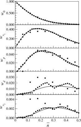
Figure 3: Zero- and one-particle weights of the cluster DM of a 5-site, cross-shaped cluster for systems of noninteracting spinless fermions with periodic boundary conditions imposed. The finite $(4,-1)\times(1,4)$ (●) and $(8,-2)\times(2,8)$ ($\blacksquare$) systems have the same shape but different sizes. The solid curves are the zero- and one-particle weights for the infinite system. For $w_{s_{1}}$, we see the finite domain effect deviations for the $(4,-1)\times(1,4)$ system is practically gone by the time we get to the $(8,-2)\times(2,8)$ system. For the rest of the one-particle weights, the finite domain effect is largely removed in the $(8,-2)\times(2,8)$ system, but shell effect persists. In fact, shell effect in $w_{d}$ is still visible when we go to the $(32,-8)\times(8,32)$ system (not shown), which has $N=1088$ sites.

We also looked at $w_{s_{1}}(\bar{n})$, which is almost unaffected by shell effect, for several systems with between 200 to 300 sites of different shapes. For systems of these sizes, the finite domain effect is negligible, but we find $w_{s_{1}}(\bar{n})$ from finite systems of different shapes differing very slightly from the infinite-system limit, and also from each other. Since we expect systems of different shapes to all approach the same infinite-system limit, we attribute these very small deviations to the shape effect. Based on more extensive numerical studies (see Chapter 4 of Ref. cheong05, ) not reported in this paper, we know that shape effect deviations are not effectively removed by the three averaging devices we have introduced in Section II.3, but fortunately these deviations are very small.

III.3 Twist Boundary Conditions Averaging

For a system of interacting spinless fermions, we cannot directly compute the exact infinite-system cluster DM. We can, however, choose to work with (i) an approximate ground-state wave function of an infinite system, or (ii) the exact ground-state wave function of a finite system, or (iii) an approximate ground-state wave function of a finite system. As reported in Section IV, we chose option (ii), where the exact ground-state wave function is obtained through numerical exact diagonalization.

Exact diagonalization severely limits the sizes of the finite systems we can work with (see Appendix of Ref. zhang03, for formula on size of Hilbert space for the strongly-interacting model given by (1)). With aggressive memory reduction measures, it is possible (but not necessarily feasible) to exactly diagonlize finite systems with up to 30 sites for all filling fractions. However, as we have illustrated in Section III.2, for systems so small, the numerical cluster DM spectra would be plagued by strong finite size effects, most notably by the shell effect. This is where twist boundary conditions averaging comes in.

Very crudely speaking, we can think of averaging numerical observables over $M$ twist boundary conditions for a finite system with $N$ sites as being equivalent to computing these numerical observables for a single finite system of $N^{*}>N$ sites, subject to only periodic boundary conditions. In the best-case scenario, the effective system size $N^{*}$ might be as large as $MN$, though $N^{*}$ will typically grow slower than $O(M)$. The computational cost of performing exact diagonalization for a system with $N$ sites over $M$ twist boundary conditions is on the order of $O(MN^{3})$, whereas the computational cost of performing exact diagonalization just once for a system with $N^{*}>N$ sites is $O({N^{*}}^{3})$. So long as the effective system size $N^{*}$ grows faster than $O(M^{1/3})$, it would be computational cheaper to employ the method of twist boundary conditions averaging, instead of exactly diagonalizing a single large finite system, to reduce finite size effects. The detail dependence of $N^{*}$ on $M$ will of course depend on the nature of the observable of interest.

From the detailed study undertaken in Appendix D of Ref. cheong05, , we know that there are cuts and cusps on the twist surface $\braket{\Psi(\phi_{x},\phi_{y})}{O}{\Psi(\phi_{x},\phi_{y})}$ of a generic observable $O$, where $\ket{\Psi(\phi_{x},\phi_{y})}$ is the many-body ground state of a finite $N$-site system subject to twist boundary conditions with twist vector $\boldsymbol{\phi}=(\phi_{x},\phi_{y})$. For non-square systems, these cusps and cuts demarcate features with a hierarchy of sizes on the twist surface. The ‘typical’ twist surface feature has a linear dimension of $2\pi/\sqrt{N}$. These are decorated by fine structures with linear dimension $2\pi/N$, which are in turn decorated by hyperfine structures with linear dimensions $2\pi/N^{2}$. The number of integration points we must use is therefore determined by what feature size we want to integrate faithfully.

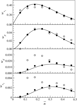
Figure 4: One-particle weights of the cluster DM of a 5-site, cross-shaped cluster within systems of noninteracting spinless fermions. The performance of twist boundary conditions averaging, using $q=16$ Monkhorst-Pack special-point integration, in reducing finite size effects for the $(4,-1)\times(1,4)$ system (●) is checked against the $(4,-1)\times(1,4)$ (○) system with periodic boundary conditions imposed. The solid curves are the cluster DM weights from the infinite system.

For the purpose of this study, we decided to integrate the fine structure on the twist surface faithfully. Therefore, we chose to average the spectrum of $\rho_{C}$ over a $q=16$ Monkhorst-Pack grid (which consists of 256 integration points in the First Brillouin Zone) for the $(4,-1)\times(1,4)$ system with $N=17$ sites. We find that twist boundary conditions averaging does indeed result in an averaged spectrum which approximates the infinite-system limit well (see Fig. 4). This averaging device, however, does not completely eliminate shell effects, as can be seen from the twist boundary conditions-averaged $w_{d}(\bar{n})$. To reduce the bias this creates for one particular choice of finite system, we combined the twist boundary conditions-averaged spectrum of $\rho_{C}$ for various finite systems. This is shown in Fig. 5. We will overlay the cluster DM spectra from several finite systems in the same way, to derive a twist boundary conditions-averaged approximation to the infinite-system cluster DM spectrum of strongly-interacting spinless fermions.

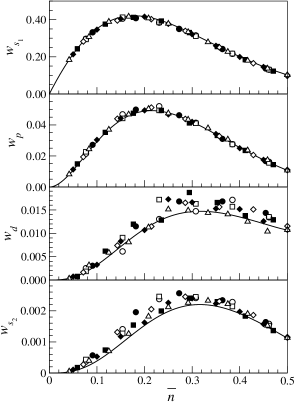
Figure 5: One-particle weights of the cluster DM of a 5-site, cross-shaped cluster, for the $(3,-2)\times(2,3)$ (●), $(4,1)\times(1,3)$ (○), $(4,-1)\times(1,3)$ ($\square$), $(4,-1)\times(1,4)$ ($\blacksquare$), $(4,-1)\times(2,3)$ ($\lozenge$), $(4,-2)\times(2,4)$ ($\blacklozenge$) and $(5,1)\times(1,5)$ ($\bigtriangleup$) systems of noninteracting spinless fermions subject to twist boundary conditions averaging, using $q=16$ Monkhorst-Pack special-point integration. Also shown are the cluster DM weights of the infinite system.

IV Strongly-Interacting System

In this section, we compute the cluster DM for interacting spinless fermions. As with the case of noninteracting spinless fermions, the cluster DM evaluated directly from the ED of various finite systems are severely affected by finite size effects. In Section III, we saw how finite size effects can be significantly reduced when the cluster DM is averaged over various twist boundary conditions, in the sense that the averaged cluster DM weights from different finite systems at various filling fractions fall close to their respective infinite-system limits. Applying twist boundary conditions averaging onto the interacting cluster DM, we find that finite size effects are reduced, but not as dramatically as for the noninteracting cluster DM. Nevertheless, the averaged cluster DM weights from different finite systems with different number of particles are sufficiently consistent with each other that we can plot a smooth curve interpolating the averaged cluster DM weights.

As explained in Section I, our interest in studying the strongly-interacting model (1) of spinless fermions with infinite nearest-neighbor repulsion is to understand how the cluster DM evolves with filling, given that we expect in this model crossovers between regimes of qualitatively different states. Furthermore, we had proposed an operator-based method of truncation which was justified by the fact that the noninteracting cluster DM is generated from a set of single-particle operators. Since we proposed the use of this truncation scheme for interacting systems, we are interested to know whether the structure of the interacting cluster DM is such that it can also be generated, perhaps approximately, from a set of single-particle operators.

To this end, we present in Sections IV.1, IV.2 and IV.3, the zero-, one- and two-particle cluster DM weights of the strongly-interacting system of spinless fermions. We check whether it is possible to: (i) write the two-particle eigenstates as the product of one-particle eigenstates; and (ii) predict the relative ordering of the two-particle weights based on the relative ordering of the one-particle weights. We then discuss in Section IV.4 whether these two criteria are met, and whether it is feasible to design an operator-based DM truncation scheme, similar to the one described in Ref. cheong04b, , for the strongly-interacting system.

IV.1 Zero-Particle Cluster DM Weight

The zero-particle cluster DM weight calculated for various finite strongly-interacting systems is shown in Fig. 6. Also shown in the figure is the zero-particle cluster DM weight of the infinite system of noninteracting spinless fermions. As we can see, the zero-particle weights of the respective systems only start differing significantly from each other for $\bar{n}>0.1$. With repulsive interacting between spinless fermions, it is more difficult in a congested system ($\bar{n}>0.2$) to form an empty cluster of sites from quantum fluctuations. As a result, the strongly-interacting $w_{0}$ falls below the noninteracting $w_{0}$. However, this fact alone does not tell us anything more about the correlations in the strongly-interacting ground state, and so we move on to consider the one-particle cluster DM weights.

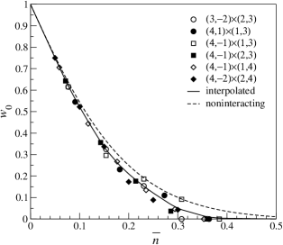
Figure 6: Zero-particle weight of the cluster DM of a 5-site, cross-shaped cluster, for the $(3,-2)\times(2,3)$ (●), $(4,1)\times(1,3)$ (○), $(4,-1)\times(1,3)$ ($\square$), $(4,-1)\times(1,4)$ ($\blacksquare$), $(4,-1)\times(2,3)$ ($\lozenge$) and $(4,-2)\times(2,4)$ ($\blacklozenge$) systems of strongly-interacting spinless fermions subject to twist boundary conditions averaging, using $q=8$ Monkhorst-Pack special-point integration. At $\bar{n}=0$ and $\bar{n}=\frac{1}{2}$, we know analytically that $w_{0}=1$ and $w_{0}=0$ respectively, and the solid ‘curve’ interpolates between these two known limits and the equally weighted data points at finite filling fractions $0<\bar{n}<\frac{1}{2}$. Also shown as the dashed curve is the zero-particle weight of the infinite system of noninteracting spinless fermions.

IV.2 One-Particle Cluster DM Eigenstates and Their Weights

In our Operator-Based DM Truncation Scheme developed in Ref. cheong04b, for a noninteracting system, the one-particle cluster DM weights play a very important role, since we select which one-particle operators to keep or discard based on the negative logarithm of these numbers. We expect the one-particle cluster DM weights, though not entirely sufficient by themselves, would also play an important role in defining an operator-based truncation scheme. Therefore, in this section, we present results for a series of calculations to determine the infinite-system limit of the one-particle cluster DM spectra for our strongly-interacting system as a function of filling fraction $\bar{n}$, and discuss their implications for an operator-based DM truncation scheme.

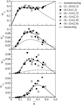
Figure 7: One-particle weights of the cluster DM of a 5-site, cross-shaped cluster within a system of strongly-interacting spinless fermions.

Though we really do need to worry about the evolution of the structure of $\ket{s_{1}}$ and $\ket{s_{2}}$ as a function of $\bar{n}$ in both the noninteracting and strongly-interacting systems, the one-particle weights are ordered by their magnitudes as $w_{s_{1}}>w_{p}>w_{d}>w_{s_{2}}$ for both systems. But while the noninteracting one-particle weights go down by roughly one order of magnitude as we go through the sequence $w_{s_{1}}\to w_{p}\to w_{d}\to w_{s_{2}}$, we see from Fig. 7 that the interacting one-particle weights decay more slowly along this same sequence.

We studied the finite $(3,-2)\times(2,3)$ (●), $(4,1)\times(1,3)$ (○), $(4,-1)\times(1,3)$ ($\square$), $(4,-1)\times(1,4)$ ($\blacksquare$), $(4,-1)\times(2,3)$ ($\lozenge$) and $(4,-2)\times(2,4)$ ($\blacklozenge$) systems subject to twist boundary conditions averaging, using $q=8$ Monkhorst-Pack special-point integration. At a filling fraction of $\bar{n}=0$, the system approaches the noninteracting limit, and thus all the one-particle weights are zero. At half-filling $\bar{n}=\frac{1}{2}$, the two-fold degenerate checker-board ground state is unaffected by twist boundary conditions averaging. We can thus perform degeneracy averaging analytically, to find that $w_{s_{1}}=\frac{1}{2}$ and $w_{p}=w_{d}=w_{s_{2}}=0$. The solid ‘curves’ in Figure 7 interpolate between these two known limits and the equally weighted data points at finite filling fractions $0<\bar{n}<\frac{1}{2}$. Also shown in Figure 7 as the dashed curves are the one-particle weights of the infinite system of noninteracting spinless fermions.

When only periodic boundary conditions are imposed, there is significantly more ‘scatter’ in the one-particle weights as a function of filling fraction $\bar{n}$, for interacting systems of different sizes, than for noninteracting systems of different sizes. Averaging the one-particle weights of the interacting systems over various twist boundary conditions visibly reduces this ‘scatter’, even though the remnant ‘scatter’ seen in Figure 7 is still rather large, compared to case for the noninteracting system (Figure 5). From our own detailed study of the method of twist boundary conditions averaging for noninteracting systems,cheong05 we know that twist boundary conditions averaging effectively removes finite size effects from some observables, but not for others. We have no reason to expect twist boundary conditions averaging to apply equally effectively over the same set of observables, when we go from noninteracting systems to interacting systems. Conversely, observables for which twist boundary conditions averaging is ineffective in noninteracting systems, might be effectively twist-boundary-conditions-averaged in interacting systems. With only input from the exact diagonalization of finite systems, and without employing system-size extrapolations, the method of twist boundary conditions averaging offers us the best hope of gaining insight into the infinite-system properties we seek.

We expect that the remnant ‘scatter’ in the twist-boundary-conditions-averaged one-particle weights will be reduced, if we had not made the nearest-neighbor repulsion infinite. There are two reasons why we did not also study the case of $t\ll V<\infty$. First, for a fixed system size $N$ and particle number $P$, the Hilbert space for the $V<\infty$ system would be much larger than that of the $V\to\infty$ system. A parallel study for $V<\infty$ of the $V\to\infty$ system sizes and particle numbers reported in this paper, with twist boundary conditions averaging, will require unacceptably long total computation time. Second, and more importantly, we believe that as long as $V/t<\infty$ is large, the qualitative implications on the Operator-Based DM Truncation Scheme would be similar to the case where $V/t\to\infty$, and therefore it suffices to examine the latter case, which is computationally much more manageable. In any case, we do not believe the remnant ‘scatter’ in the twist-boundary-conditions-averaged DM weights will hamper our efforts in drawing qualitative conclusions regarding the applicability, or otherwise, of the Operator-Based DM Truncation Scheme for interacting Fermi liquids.

In the Operator-Based DM Truncation Scheme described in Ref. cheong04b, , we discard one-particle cluster DM eigenstates with very small weights, and keep only the many-particle cluster DM eigenstates built from the retained one-particle eigenstates. The sum of weights of the truncated set of cluster DM eigenstates will then be very nearly one, if the discarded one-particle weights are all very small compared to the maximum one-particle weight. As we can see from Fig. 7, the ratio of the largest one-particle weight, $w_{s_{1}}$, to the smallest one-particle weight, $w_{s_{2}}$, is not large enough for us to justify keeping $\ket{s_{1}}$ and discarding $\ket{s_{2}}$, except when the system is very close to half-filled.

We believe that the one-particle cluster DM weights are so close to each other in magnitude, because of the net ‘strength’ of interactions straddling the cluster and its environment is strong compared to the net ‘strength’ of interactions strictly within the cluster. Unfortunately for our five-site cluster, which was chosen because it is the smallest non-trivial cluster having the full point group symmetry of the underlying square lattice, the sites within the cluster are poorly connected, i.e. a cluster site is on average connected to more environmental sites than to other cluster sites. To have more of the total interactions of the cluster with the system be confined within the cluster, a cluster significantly larger than the five-site cluster studied in this paper will be needed. This large cluster must then be embedded in a finite system that is larger still, making exact diagonalization studies unfeasible.

IV.3 Two-Particle Cluster DM Eigenstates and Their Weights

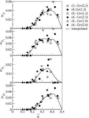
Figure 8: Two-particle weights of the cluster DM of a 5-site, cross-shaped cluster within a system of strongly-interacting spinless fermions.

While it is desirable to have a broader distribution of one-particle weights, our more important task is to examine how closely the many-particle cluster DM eigenstates can be approximated as products of one-particle cluster DM eigenstates. In particular, we look at the two-particle cluster DM eigenstates, and find that of the two-particle states listed in (28), the only states which are allowed by the no-nearest-neighbor constraint to appear in the cluster Hilbert space are $\ket{S}$, $\ket{P_{\pm}}$, $\ket{P^{\prime\prime}_{\pm}}$ and $\ket{D}$. We know therefore that the two-particle sector of $\rho_{C}$ comprises a $1\times 1$ $S$-diagonal block (with weight $w_{S}$), a $1\times 1$ $D$-diagonal block (with weight $w_{D}$), and two degenerate $2\times 2$ $P$-diagonal blocks (with weights $w_{P_{1}}$ and $w_{P_{2}}$). The two-particle weights are shown as a function of filling $\bar{n}$ in Fig. 8.

For the finite $(3,-2)\times(2,3)$ (●), $(4,1)\times(1,3)$ (○), $(4,-1)\times(1,3)$ ($\square$), $(4,-1)\times(1,4)$ ($\blacksquare$), $(4,-1)\times(2,3)$ ($\lozenge$) and $(4,-2)\times(2,4)$ ($\blacklozenge$) systems studied, subject to twist boundary conditions averaging, using $q=8$ Monkhorst-Pack special-point integration, all the two-particle weights are zero at $\bar{n}=0$ as the systems approach the noninteracting limit. At half-filling $\bar{n}=\frac{1}{2}$, we again perform degeneracy averaging analytically on the two-fold degenerate checker-board ground state to find that all the two-particle weights are zero. In Figure 8, the solid ‘curves’ interpolates between these two known limits and the equally weighted data points at finite filling fractions $0<\bar{n}<\frac{1}{2}$.

We realized that there are significantly fewer nontrivial two-particle eigenstates of $\rho_{C}$ than predicted from the combination of one-particle eigenstates. From the point of view of implementing the Operator-Based DM Truncation Scheme, this poses no problem if the non-occurring two-particle states are predicted to have small enough weights that they will be excluded by the truncation scheme. However, we find that this is not the case. For example, the two-particle state $\ket{S^{\prime}}$, which does not occur, is predicted by simple combination of the one-particle states $\ket{s}$ and $\ket{\bar{s}}$ to have a weight comparable to that of the two-particle state $\ket{S}$, which does occur.

Of the two-particle weights that are allowed by the no-nearest-neighbor constraint, we expect their weights to follow the sequence $w_{P_{1}}\gtrsim w_{D}>w_{S}$, if they can indeed to thought of products of one-particle states. From Fig. 8, we indeed observe this sequence of two-particle weights, even though their actual magnitudes (calculated as the product of one-particle weights divided by the zero-particle weight) do not come out right. This observation is encouraging, because we might yet be able to push a variant of the Operator-Based DM Truncation Scheme through, by introducing constraints on how many-particle cluster DM states can be built up from one-particle cluster DM states.

IV.4 Signatures of Fermi-Liquid Behaviour in the Cluster DM

Over broad ranges of filling fractions, the ground state of our strongly-interacting model (1) of spinless fermions is expected to be an interacting Fermi liquid. While we understand the cluster DM structure of a noninteracting Fermi liquid completely, we do not yet understand how an interacting Fermi liquid will manifest itself in the structure of its cluster DM. Unlike a noninteracting Fermi liquid, the ground-state DM of an interacting Fermi liquid will not simply be the exponential of a noninteracting pseudo-Hamiltonian. Nevertheless, we expect that the interacting pseudo-Hamiltonian $\tilde{H}$ appearing in the interacting Fermi-liquid ground-state DM $\rho=\exp(\tilde{H})$ can be made to look like the sum of a noninteracting pseudo-Hamiltonian $\tilde{H}_{0}$, and a much weaker interaction term $\tilde{H}_{1}$, by a canonical transformation. From Landau’s Fermi liquid theory, we know that such a canonical transformation (similar to the one which relates Landau quasi-particles to bare fermions) works by burying much of the bare interactions within the quasi-particles.

In tracing down the ground-state DM, our hope then is that the cluster DM can also be written, after a canonical transformation local to the cluster, as the exponential of the sum of a noninteracting pseudo-Hamiltonian $\tilde{H}_{C,0}$ (which is perhaps related to $\tilde{H}_{0}$ in the same way as for the noninteracting Fermi liquid), and a weak interaction term $\tilde{H}_{C,1}$. We suspect that the criterion for this to be possible is that we must be able to construct approximate quasi-particles using only cluster states to absorb the bare interactions. However, we also believe that the requirement that the canonical transformation act strictly within the cluster will fail to completely incorporate interactions that straddle the cluster and its environment.

In Section IV.3, we found that for our strongly-interacting system, the two-particle cluster DM eigenstates look nothing like simple products of two one-particle cluster DM eigenstates each. In fact, many combinations of two one-particle cluster DM eigenstates give invalid two-particle cluster states that violate the condition of no-nearest-neighbor occupation. It is tempting, based on this observation, to say then that the cluster DM is not the exponential of an approximately noninteracting pseudo-Hamiltonian. However, it must be remembered that in an interacting Fermi liquid, the quasi-particles are also not single bare particles. Instead, they are superpositions of states containing different number of bare particles, which leads us to think of a quasi-particle as a bare particle being screened by other bare particles in its vicinity.

With this in mind, we realized that to identify the quasi-particle structure of the cluster DM, we need to construct appropriate linear combinations of the $P$-particle cluster DM eigenstates, so that the cluster DM, when written in terms of these ‘quasi-particles’, look like the exponential of a noninteracting pseudo-Hamiltonian $\tilde{H}_{C,0}$ plus a weak interaction term $\tilde{H}_{C,1}$. This involves writing the pseudo-Hamiltonian $\tilde{H}_{C}$ as a sum of terms, representing the independent quantum fluctuations associated with each of the quasiparticles. This can be accomplished by defining an operator singular value decomposition of the cluster DM with respect to an appropriate operator norm, which forms the basis for judging whether the quantum fluctuations associated with two linear combination of bare operators are independent. Details of such an operator singular value decomposition will be reported in a future paper.cheong07

V Summary & Discussions

To summarize, we have calculated numerically the cluster DM for a cross-shaped cluster of five sites within both a system of noninteracting spinless fermions described by the Hamiltonian (29), and a system of strongly-interacting spinless fermions described by the Hamiltonian (1). For the noninteracting system, the cluster DM was obtained from the cluster Green-function matrix using the exact formula (30) obtained in Ref. cheong04a, , whereas for the interacting system, the cluster DM was obtained from the exact-diagonalization ground-state wave function by tracing down degrees of freedom outside of the cluster. For the purpose of making the comparison of the cluster DM spectra more straightforward, we worked with the same collection of finite non-square systems for interacting and noninteracting spinless fermions.

To make the results of this comparison less dependent on the geometry of the finite systems chosen, degeneracy averaging followed by orientation averaging of the cluster DM spectra were carried out. When combined, these two averaging apparatus has the effect of restoring full square-lattice symmetry to the cluster DM. We also analyzed in detail the finite size effects not removed by degeneracy and orientation averaging, by inspecting the numerical cluster DM spectra coming from finite noninteracting systems of various sizes. By increasing the system size systematically, we find visually that the infinite-system limit of the cluster DM is ‘attained’ when the system size reaches a couple of hundred sites.

Noting that these are forbiddingly large system sizes to work with for interacting systems, where the ground-state wave functions have to be obtained via exact diagonalization, we then tested the apparatus of twist boundary conditions averaging on finite systems with between 10 and 20 sites. For noninteracting spinless fermions, we find that the twist boundary conditions-averaged cluster DM weights for different finite systems and different filling fractions indeed fall close to the various infinite-system limits. Since we do not perform system-size extrapolations, we interpolate between the degeneracy-, orientation-, and twist boundary conditions-averaged cluster DM weights for the various finite interacting systems and their respective accessible filling fractions, and take the result curves to be our best approximation of the cluster DM spectrum of the infinite interacting system.

Comparing the twist boundary conditions-averaged cluster DM spectra for the noninteracting and strongly-interacting systems, we find similar qualitative behavior in the zero-particle weights as functions of filling fraction, and qualitatively different behaviours in the one-particle weights as functions of filling fraction. However, the relative ordering $w_{s_{1}}>w_{p}>w_{d}>w_{s_{2}}$ is the same at all $\bar{n}<\frac{1}{2}$ for both systems. Quantitatively, we find for noninteracting spinless fermions that the one-particle weights go down by roughly one order of magnitude each time as we go through the sequence $w_{s_{1}}\to w_{p}\to w_{d}\to w_{s_{2}}$. For strongly-interacting spinless fermions, the one-particle weights decay much more slowly along the sequence.

The implications this observation have for the Operator-Base DM Truncation Scheme developed in Ref. cheong04b, is that, for a small fixed fraction of one-particle eigenstates retained, the total cluster DM weight of eigenstates retained would be much smaller for the strongly-interacting system compared to the noninteracting system, since the ratio of the smallest to the largest one-particle weights, $w_{s_{2}}/w_{s_{1}}$, is not very much smaller than one. This narrow distribution of one-particle cluster DM weights aside, we observed that the relative ordering $w_{P_{1}}\gtrsim w_{D}>w_{S}$ of the two-particle cluster DM weights, predicted based on the combination of one-particle cluster DM weights, is confirmed numerically — even though the predicted weights are off. This suggests that we might be able to push a variant of the naive Operator-Based DM Truncation Scheme through, by introducing additional rules on how one-particle cluster DM eigenstates can be combined to give only the valid many-particle cluster DM eigenstates. We did not attempt to implement such a truncation scheme, and test how badly its numerical accuracy is affected by the ratio $w_{s_{2}}/w_{s_{1}}$ (by calculating the dispersion relation, for example, as was done in Ref. cheong04b, ), because we feel that such a naive scheme was not in the spirit of finding an appropriate ‘quasi-particle’ description for the low-energy excitations of our system of interacting spinless fermions given by (1).

Finally, we realized that our numerical studies do not allow us to conclude whether the cluster DM of the interacting system furnishes a good ‘quasi-particle’ description for the strongly-interacting system. To be able to check this, we must be able to construct appropriate superpositions of cluster DM eigenstates with different particle numbers, so that the pseudo-Hamiltonian $\tilde{H}_{C}\sim\log\rho_{C}$ looks like the sum of a noninteracting pseudo-Hamiltonian $\tilde{H}_{C,0}$ and a weak interacting pseudo-Hamiltonian $\tilde{H}_{C,1}$. Instead of a simple eigenvalue problem for the cluster DM, the problem of discovering what ‘quasi-particle’ operators make up the cluster DM is an operator singular value decomposition problem. We will carefully define this operator singular value decomposition in a future paper, and describe how it can be applied to the density matrix of two disjoint clusters to systematically extract operators associated with independent quantum fluctuations within each cluster, and their inter-cluster correlations.cheong07

Appendix A Computational Complexity of Cluster Density-Matrix Calculation

In this appendix we compare the naive algorithm and the pre-sorted inner product algorithm, based on (10) and (11) respectively, for numerically computing the cluster density matrix, and determine their computational complexities. To begin, we denote by $D(P)$ the size of the system Hilbert space with $P$ particles, $D_{C}(P_{C})$ the size of the cluster Hilbert space with $P_{C}$ particles, and $D_{E}(P_{C})$ the size of the environment Hilbert space with $P_{E}=P-P_{C}$ particles. Noting that there can be no matrix elements between cluster configurations with different number of particles, we calculate each $P_{C}$ sector of the cluster DM separately. To keep our notations compact, let us drop the $P$ and $P_{C}$ dependences in $D(P)$, and $D_{C,E}(P_{C})$ respectively from this point onwards, and reinstate these dependences only when necessary. Readers are referred to Appendix A in Ref. cheong05, for more technical details on the computational implementation of this trace-down calculation of the cluster DM.

In the naive algorithm based on (10), the cluster DM matrix elements are computed by starting nested ‘for’ loops in $\mathbf{l}$ and $\mathbf{l}^{\prime}$, each running over $D_{C}$ indices. For each pair of cluster configurations $\ket{\mathbf{l}}$ and $\ket{\mathbf{l}^{\prime}}$, one would need to then determine which of the $P$-particle configurations $\ket{\mathbf{j}}$ contain the two cluster configurations. This involves running through the $D$ configurations in the system Hilbert space, and for each configuration, comparing the $P$ occupied sites with the $P_{C}$ occupied sites in the cluster configurations $\ket{\mathbf{l}}$ and $\ket{\mathbf{l}^{\prime}}$. The computational effort incurred for this matching is thus $O(DP)$. Two vectors of indices, $\mathbf{i}$, whose entries are the indices of system configurations $\ket{\mathbf{j}}$ giving cluster configuration $\ket{\mathbf{l}}$, and $\mathbf{i}^{\prime}$, whose entries are the indices of system configurations $\ket{\mathbf{j}}$ giving cluster configuration $\ket{\mathbf{l}^{\prime}}$, are obtained. The lengths of these index vectors vary, but are of $O(D_{E})$. One can then compare the two index vectors, at a computational cost of $O(D_{E}^{2})$, to find which pairs of system configurations giving cluster configurations $\ket{\mathbf{l}}$ and $\ket{\mathbf{l}^{\prime}}$ share the same environment configuration. Following this, one can sum over the amplitude of such pairs, at a computational cost of $O(D_{E})$, to obtain the cluster DM matrix element $\braket{\mathbf{l}}{\rho_{C}}{\mathbf{l}^{\prime}}$. For this naive algorithm, the net computational effort is on the order of $D_{C}^{2}(DP+D_{E}^{2}+D_{E})\sim D_{C}^{2}(DP+D_{E}^{2})$.

In the pre-sorted inner-product algorithm based on (11), we need to first run through $D$ system configurations to pre-sort the amplitudes in the ground-state wave function. For each system configuration $\ket{\mathbf{j}}$, we determine at a computational cost of $P$ comparisons what cluster configuration $\ket{\mathbf{l}}$ and environment configuration $\ket{\bm{missing}}$ it contains. We then search through the cluster and environment Hilbert spaces to determine what the indices of $\ket{\mathbf{l}}$ and $\ket{\bm{missing}}$ are in their respective Hilbert spaces, which incurs a computational effort on the order of $D_{C}P_{C}$ and $D_{E}P_{E}$ respectively. Once these indices are determined, the amplitudes in the ground-state wave function are organized into a $D_{C}\times D_{E}$ matrix. The net computational expenditure is thus on the order of $D(P+D_{C}P_{C}+D_{E}P_{E})\sim D(D_{C}P_{C}+D_{E}P_{E})$. After sorting the ground-state wave function, we can then start nested for loops in $\mathbf{l}$ and $\mathbf{l}^{\prime}$, each running over $D_{C}$ indices, to evaluate the matrix element $\braket{\mathbf{l}}{\rho_{C}}{\mathbf{l}^{\prime}}$ as the inner product between two vectors of length $D_{E}$. This trace-down stage incurs a computational cost of $O(D_{C}^{2}D_{E})$. Overall, the computational cost is on the order of $D(D_{C}P_{C}+D_{E}P_{E})+D_{C}^{2}D_{E}$.

For models allowing nearest-neighbor occupation, the system Hilbert space is the direct product of the cluster Hilbert space and the environment Hilbert space, i.e. $D=D_{C}D_{E}$. Since the number $P$ of particles is small in any reasonable exact diagonalization, we can treat it as a $O(1)$ constant. For small clusters, the size $D_{C}$ of the cluster Hilbert space will also be small, so that the size $D_{E}$ of the environment Hilbert space will be comparable in magnitude to $D$. With these considerations, we find that the computational cost for the naive algorithm is $O(DD_{C}^{2}+D_{C}^{2}D_{E}^{2})\sim O(D^{2})$, while the computational cost for the inner-product algorithm with pre-sorting is $O(D+DD_{E}+D_{E})\sim O(D^{2})$. The efficiency of the two algorithms therefore depend on the prefactors, the estimation of which requires more thorough analyses of the two algorithms.

For a model such as (1), where nearest-neighbor occupation is forbidden, the system Hilbert space is smaller than the direct product of the cluster Hilbert space and the environment Hilbert space, i.e. $D<D_{C}D_{E}$. Given again that $P$ and $D_{C}$ are small numbers, the computational cost for the two algorithms are essentially determined by the ratio $D_{C}D_{E}/D$. This ratio is strongly dependent on the dimensionality of the problem: the superfluous configurations generated by the direct product of the cluster Hilbert space and the environment Hilbert space are invalid because they contain nearest-neighbor sites, right at the boundary between the cluster and its environment, which are occupied. In one dimension, the number of superfluous configurations is small, because the boundary between the cluster and its environment consists only of two bonds, whatever the size $N_{C}$ of the cluster. In two dimensions, the boundary between the cluster and its environment is a line cutting roughly $\sqrt{N_{C}}$ bonds. The number of superfluous configurations is then proportional to $\exp(\alpha_{2}\sqrt{N_{C}})$, where $\alpha_{2}$ is a constant prefactor which depends on the shape of the cluster. In $d$ dimensions, the number of boundary bonds is on the order of $N_{C}^{(d-1)/d}$, and the number of superfluous states is proportional to $\exp(\alpha_{d}N_{C}^{(d-1)/d})$. Therefore, in dimensions greater than one, $D_{C}D_{E}$ become increasingly larger than $D$ as $N_{C}$ is increased, and the inner-product algorithm with pre-sorting, which involves only one power of $D_{C}D_{E}$, is more efficient than the naive algorithm, which involves $(D_{C}D_{E})^{2}$.

References

- (1) S. R. White, Phys. Rev. Lett. 69, 2863 (1992); Phys. Rev. B 48, 10345 (1993).
- (2) F. Verstraete, D. Porras, and J. I. Cirac, Phys. Rev. Lett. 93, 227205 (2004); F. Verstraete and J. I. Cirac, cond-mat/0407066 (2004).
- (3) C. Morningstar and M. Weinstein, Phys. Rev. D 54, 4131 (1996); E. Altman and A. Auerbach, Phys. Rev. B 65, 104508 (2002); E. Berg, E. Altman, and A. Auerbach, Phys. Rev. Lett. 90, 147204 (2003); R. Budnik and A. Auerbach, Phys. Rev. Lett. 93, 187205 (2004); S. Capponi, A. Läuchli, and M. Mambrini, Phys. Rev. B 70, 104424 (2004).
- (4) S. Furukawa, G. Misguich, and M. Oshikawa, cond-mat/0508469 (2005).
- (5) S.-A. Cheong and C. L. Henley, Phys. Rev. B 69, 075111 (2004).
- (6) M. C. Chung and I. Peschel, Phys. Rev. B 64, 064412 (2001).
- (7) S.-A. Cheong and C. L. Henley, Phys. Rev. B 69, 075112 (2004).
- (8) C. L. Henley and N. G. Zhang, Phys. Rev. B 63, 233107 (2001).
- (9) N. G. Zhang and C. L. Henley, Phys. Rev. B 68, 014506 (2003).
- (10) N. G. Zhang and C. L. Henley, Eur. Phys. J. B 38, 409 (2004).
- (11) S.-A. Cheong, Ph.D. thesis, Cornell University, 2006.
- (12) G. Spronken, R. Jullien and M. Avignon, Phys. Rev. B 24, 5356 (1981); X. Zotos, P. Prelovšek and I. Sega, Phys. Rev. B 42, 8445 (1990); D. Poilblanc and E. Dagotto, Phys. Rev. B 44, R466 (1991); D. Poilblanc, Phys. Rev. B 44, 9562 (1991); C. Gros, Z. Phys. B – Condensed Matter 86, 339 (1992); J. T. Gammel, D. K. Campbell and E. Y. Loh, Jr., Synth. Met. 57, 4437 (1993); C. Lin, F. H. Zong, and D. M. Ceperley, Phys. Rev. E 64, 016702 (2001).
- (13) H. J. Monkhorst and J. D. Pack, Phys. Rev. B 13, 5188 (1976); D. J. Chadi, Phys. Rev. B 16, 1746 (1977); J. D. Pack and H. J. Monkhorst, Phys. Rev. B 16, 1748 (1977).
- (14) Eric W. Weisstein. “Dihedral Group D4.” From MathWorld — A Wolfram Web Resource, http://mathworld.wolfram.com/DihedralGroupD4.html; M. Lax, Symmetry Principles in Solid State and Molecular Physics (Dover (Mineola, New York), 2001); J. M. Hollas, Modern Spectroscopy, Third Edition (John Wiley & Sons (Chichester), 1996).
- (15) S.-A. Cheong and C. L. Henley, in preparation.