Non-perturbative behavior of the quantum phase transition to a nematic Fermi fluid

Abstract

We discuss shape (Pomeranchuk) instabilities of the Fermi surface of a two-dimensional Fermi system using bosonization. We consider in detail the quantum critical behavior of the transition of a two dimensional Fermi fluid to a nematic state which breaks spontaneously the rotational invariance of the Fermi liquid. We show that higher dimensional bosonization reproduces the quantum critical behavior expected from the Hertz-Millis analysis, and verify that this theory has dynamic critical exponent $z=3$. Going beyond this framework, we study the behavior of the fermion degrees of freedom directly, and show that at quantum criticality as well as in the the quantum nematic phase (except along a set of measure zero of symmetry-dictated directions) the quasi-particles of the normal Fermi liquid are generally wiped out. Instead, they exhibit short ranged spatial correlations that decay faster than any power-law, with the law $|x|^{-1}\exp(-\textrm{const.}\;|x|^{1/3})$ and we verify explicitely the vanishing of the fermion residue utilizing this expression. In contrast, the fermion auto-correlation function has the behavior $|t|^{-1}\exp(-{\rm const}.\;|t|^{-2/3})$. In this regime we also find that, at low frequency, the single-particle fermion density-of-states behaves as $N^{*}(\omega)=N^{*}(0)+B\;\omega^{2/3}\log\omega+\ldots$, where $N^{*}(0)$ is larger than the free Fermi value, $N(0)$, and $B$ is a constant. These results confirm the non-Fermi liquid nature of both the quantum critical theory and of the nematic phase.

I Introduction

The behavior of interacting Fermi systems near continuous quantum phase transitions is a central problem in the physics of strongly correlated systems. Although much work has been done on this subject, there are still many open and as yet unresolved questions. At present the standard theory of quantum phase transitionsHertz (1976); Millis (1993); Sachdev (1999) relies primarily on an analysis on the effects of fluctuations perturbatively about the results of Hartree-Fock theory. This analysis proceeds in almost complete analogy with the theory of classical critical phenomena about its upper critical dimension, and its straightforward extension to quantum phase transitions. In practice it consists of an effective theory for a suitable order parameter field while other degrees of freedom, including fermions, are often integrated out at the outset.

In many cases of interest the systems are metallic and have gapless fermionic excitations. In the standard approach, their net effect is to introduce damping in the collective modes associated with the order parameter field. In practice this results in the introduction of dissipative terms in the effective action. While much of this is certainly correct, this approach implicitly assumes that the fermions are largely unaffected by quantum criticality. Why this should be the case is far from obvious.

The assumptions of the Landau theory of the Fermi liquidPines and Nozières (1966,1989); Abrikosov et al. (1963); Baym and Pethick (1991) are self-consistent and well justified within the Landau phase which has a sizable basin of stability, except in one dimensional systemsShankar (1994); Polchinski (1994); Luther (1979); Haldane (1992, 1994); Castro Neto and Fradkin (1994a, b); Castro Neto and Fradkin (1995); Houghton and Marston (1993); Houghton et al. (2000). However, there is no reason for these assumptions to hold outside the Landau phase. However, there is also mounting evidence that these assumptions may also not hold in a number of phases (and not just at quantum critical points), including ferromagnetic metalsChubukov (2005) and nematic phases of Fermi fluidsOganesyan et al. (2001); Metzner et al. (2003). The possibility that quantum criticality may lead to non-Fermi liquid behavior has been a focus of research in recent years, primarily (but not only) in connection with the physics of the “normal phase” of high temperature superconductorsChubukov et al. (1994); Sachdev (1999); Varma (1996); Chakravarty et al. (2001), and with heavy-fermion systemshea .

The simplest example where the Landau assumptions on the behavior of the quasiparticles are violated is the quantum phase transition from a normal (Landau) Fermi liquid phase to a nematic Fermi fluid Oganesyan et al. (2001). A nematic Fermi fluid is a uniform phase of a system of interacting fermions in which the shape of the Fermi surface is distorted spontaneously, thus breaking rotational invariance.com (a) This state is an example of the fate of a Fermi liquid beyond a Pomeranchuk instabilityPomeranchuk (1958). In this case, the Landau assumptions appear to be violated throughout this phase, and not just at the quantum critical point.Oganesyan et al. (2001); Metzner et al. (2003)

The clearest experimental evidence to date of a nematic Fermi fluid phase has been found in very clean two-dimensional electron gases in magnetic fields in ultra-clean samples.Lilly et al. (1999); Du et al. (1999) The striking resistivity anisotropies that are observed in these experiments can be explained by the onset of nematic order at low temperatures.Fradkin and Kivelson (1999) It has also been proposed that phases of this type may play a central role on the physics of high temperature superconductors.Kivelson et al. (1998, 2003) This charge-ordered state of a strongly correlated system of fermions is the simplest example of an electronic liquid crystal phaseKivelson et al. (1998).

The problem of the fate of the fermions at quantum criticality, and in the “non-Fermi liquid” phases mentioned above, so far has only been considered within perturbative corrections to Hartree-Fock/RPA theory. Oganesyan, Kivelson and FradkinOganesyan et al. (2001) found that the quasiparticles are wiped out as well defined quantum states. This is due to the large fluctuations of (overdamped) quadrupolar collective modes. These authors found, within a Hartree-Fock and RPA theory, an overdamped collective mode with $z=3$ at the critical point. They also found that the fermion self-energy acquires, at the quantum critical point, an imaginary part with a frequency dependence following the law $\omega^{2/3}$. A similar behavior has been found in the case of the Stoner transition and in the antiferromagnetic phaseVekhter and Chubukov (2004); Chubukov (2005). Oganesyan and coworkers also found that this behavior holds inside the nematic phase, except along a set of measure zero of directions determined by the symmetry breaking.com (b) However, it seems quite likely that such leading order behaviorOganesyan et al. (2001); Metzner et al. (2003) may actually signal the complete failure of the Landau theory of the Fermi liquid. It is clear that to better understand this problem a non-perturbative analysis of the behavior of the fermions at the quantum phase transitions (and beyond) is needed. ChubukovChubukov (2005) has given arguments which, in the context of the ferromagnetic metallic transition, suggest that this behavior may persist beyond the lowest order in perturbation theory.

In this paper we will consider the nematic quantum phase transition in Fermi fluids using the non-perturbative approach of higher dimensional bosonizationHaldane (1992); Castro Neto and Fradkin (1994a); Houghton and Marston (1993). We will not discuss the (important) lattice effects here. Bosonization is a powerful tool to study the non-perturbative behavior of one-dimensional gapless Fermi systems, the best understood fermionic quantum critical systemsEmery (1979). As it is well known, the kinematics of one-dimensional systems is so constrained that the bosonic collective modes completely exhaust the spectrum of these fermionic systems, allowing even for a full reconstruction of the fermionic operators entirely in terms of bosons. A striking result if one-dimensional system is that the electron acquires a non-trivial anomalous dimension and it is no longer the quasiparticle of these systems, even for arbitrarily weak interactions. For these reasons one-dimensional gapless Fermi systems have been termed ‘Luttinger liquids’. The actual quasiparticles are non-trivial solitons which are orthogonal to a bare electron.Haldane (1981)

In dimensions higher than one the physics (and the kinematics) is quite different than in one dimension. Nevertheless bosonization methods still yield the physics of the Landau theory of the Fermi liquid correctly.Haldane (1992); Castro Neto and Fradkin (1994a); Houghton and Marston (1993) Superficially this may seem surprising since in dimensions higher than one there are no longer strong kinematic constraints, and consequently the bosonic collective modes cannot exhaust the spectrum of an interacting Fermi system. Instead, except for narrow regimes in which the collective modes are stable quantum states, they exhibit Landau damping, reflecting their decay into particle-hole pairs. It is a key check of the validity of higher dimensional bosonization that it gets the physics of Landau damping.Castro Neto and Fradkin (1994b)

One appealing feature of higher dimensional bosonization is that it is actually a theory of the quantum fluctuations of the shape of the Fermi surface. It is thus a natural approach to study quantum phase transitions associated with Pomeranchuk instabilities, and in particular the nematic state.Barci and Oxman (2003) More specifically, we focus on the nematic case for spinless fermions and compare with the work of Oganesyan and coworkersOganesyan et al. (2001) based on RPA and Hartree-Fock. We find that the physics of the bosonic collective modes is the same in bosonization and in RPA, and thus our results agree with those of Ref.[Oganesyan et al., 2001] in the Landau phase, in the nematic phase and at the quantum critical point. Perhaps, this is not so surprising since at long wavelengths RPA becomes asymptotically exact and this is the regime in which bosonization is correct (for a more thorough discussion, see Metzner et. al., 2005). In particular we derive the effective action near the quantum critical point and find that it does have a Hertz-Millis form with dynamic critical exponent $z=3$, consistent with the findings Oganesyan and coworkersOganesyan et al. (2001), and by Nilsson and Castro NetoNilsson and Castro Neto (2005), but in disagreement with the results of K. YangYang (2005).

We further use bosonization methods to obtain the fermion propagator. This result is well beyond the Hartree-Fock/RPA theory and thus it allows us to study the fate of the fermions non-perturbatively. We find striking violations of the Landau assumptions for Fermi liquids. Thus, the equal-time behavior of the fermion propagator at the quantum critical point (at zero temperature) is found to fall off faster than any power, decaying instead with a law $\frac{1}{|x|}\;\exp(-{\rm const}.\;|x|^{1/3})$ as a function of distance. The same behavior is found in the nematic phase except along symmetry-determined directions. We also verify explicitely from this expression the vanishing of the fermion residue as expected from this kind of behavior. In contrast to the equal-time behavior, at quantum criticality the fermion auto-correlation function behaves as $\frac{1}{|t|}\;\exp(-{\rm const}.\;|t|^{-{2/3}})$, with a similar albeit anisotropic law in the nematic phase as well. We also find that the low energy behavior of the one-particle density of states $N^{*}(\omega)$ exhibits an enhancement to a zero frequency value $N^{*}(0)$ which we find to be larger than $N(0)$, its non-interacting value. At finite but low frequency we further find that this one-particle density of states behaves as $N^{*}(\omega)=N^{*}(0)+B\;\omega^{2/3}\ln\omega$ ($B$ is a constant), i.e. a cusp at $\omega=0$.

Thus, our bosonization results confirm that the nematic phase of a Fermi fluid is a non-Fermi liquid. However, its behavior is more complex than the predictions of the Hartree-Fock/RPA theory. Recently ChubukovChubukov (2005) has examined the behavior of the fermion self-energy in perturbation theory at the ferromagnetic quantum critical point and found that the frequency-dependence is not changed by higher order corrections. Our results for the auto-correlation function are consistent with his results, as well as with Refs.[Oganesyan et al., 2001] and [Metzner et al., 2003; Dell’Anna and Metzner, 2005]. However we also find that the equal-time propagator (the “one-particle density matrix”) has a very different behavior than what is predicted from these diagrammatic methods.

The paper is organized as follows: In section II we derive a theory of the nematic QCP via higher dimensional bosonization. Here we present a theory of the quantum phase transition to the nematic Fermi fluid, section II.1, and show that it reproduces the analog of Hertz-Millis theory for this problem. In particular we give a detailed analysis of the spectral functions of the collective modes, section II.2, and derive the effective action valid in the vicinity of the quantum phase transition, section II.3. In section III we use bosonization methods to calculate the fermion propagator. Here we extract the full diagrammatic perturbation theory of the fermion Green function from bosonization, and use it to calculate the fermion self-energy. Here we check that the bosonization formulas reproduce correctly the non-Fermi liquid behavior found within the Hartree-Fock/RPA theoryOganesyan et al. (2001). We then use the full bosonized expression for the fermion propagator. Here we find large violations to Fermi liquid theory both at quantum criticality and in the nematic Fermi fluid phase. As an application we give a calculation of the fermion one-particle density of states. Finally, in section IV we draw our conclusions. To help keep this paper self contained, in Appendix A we give a short review the extension of bosonization to $D$-dimensional Fermi systems. (For a more in depth review, see Ref.[Houghton et al., 2000]). In Appendix B we summarize details of the effective quadrupolar interactions, including fermion screening and Landau damping effects. In Appendix C we discuss the effects of the (uncondensed) s-wave channel on the effective theory for the nematic. The details of the calculation of the boson propagators are given in Appendix D.

II The nematic quantum phase transition and the order parameter

In this section, we consider the boson theory, obtained via an extension of bosonization to greater than one dimension, near a nematic (Pomeranchuk) instability of a translationally invariant fermion system. In the notation of Appendix A, we take the following action for the bosons

$$S_{0}=\frac{N(0)}{2}\sum_{S}\!\int d^{2}xdt\bigg{[}-\partial_{t}\varphi_{S}{\bf v}_{S}\cdot\nabla\varphi_{S}-\big{(}{\bf v}_{S}\cdot\nabla\varphi_{S}\big{)}^{2}\bigg{]}$$ (1)

and forward scattering interactions

$$S_{\rm int}=\frac{N(0)}{2}\sum_{S,T}\int d^{2}xd^{2}x^{\prime}dt\;F_{S-T}({\bf x-x^{\prime}}){\bf v}_{S}\cdot\nabla\varphi_{S}({\bf x}){\bf v}_{T}\cdot\nabla\varphi_{T}({\bf x^{\prime}})$$ (2)

Here, $S$ labels the patch defined by coarse graining the Fermi surface, and the density of quasiparticles in a patch may be obtained from the boson field $\varphi_{S}({\bf x},t)$ via the relation $\delta n_{S}({\bf x},t)=N(0){\bf v}_{S}\cdot\nabla\varphi_{S}({\bf x},t)$. $F_{S-T}({\bf x}-{\bf x}^{\prime})$ is therefore the interaction between particle-hole pairs in patches $S$ and $T$.

We begin by analyzing our bosonized theory for a constant field configuration and reproduce Pomeranchuk’s result. Consider configurations such that $\delta n_{S}$ is constant in space and time over some particular range of time T. The resulting action is:

$$S_{\text{shape}}=-\frac{VT}{N(0)}\left(1+F_{0}\right)\left(m_{0}^{+}\right)^{2}\\ -\frac{VT}{2N(0)}\sum_{\ell>0}^{N/2}\left(1+F_{\ell}\right)\left(\left(m_{\ell}^{+}\right)^{2}+\left(m_{\ell}^{-}\right)^{2}\right)$$ (3)

where we have expanded $\delta n_{S}$ as:

$$\delta n_{S}=\sqrt{\frac{2}{N}}\sum_{\ell=0}^{N/2}\left[m_{\ell}^{+}\cos(\ell\theta_{S})+m_{\ell}^{-}\sin(\ell\theta_{S})\right]$$ (4)

and introduced the Fermi liquid parameters via

$$F_{S-T}=\frac{1}{N}F_{0}+\frac{2}{N}\sum_{\ell>0}F_{\ell}\cos\ell\left(\theta_{S}-\theta_{T}\right)$$ (5)

Hence, for arbitrary $m_{\ell}^{\pm}$, we find that any $F_{\ell}<-1$ will destabilize the Fermi liquid. The point $F_{\ell}=-1$ we shall call the Pomeranchuk (nematic for $\ell=2$) quantum critical point (QCP). Though Fermi liquid theory breaks down at this point, Luttinger’s theorem is still obeyed.

It should also be noted that in the above analysis we could have included interactions involving large angle scattering (which may lead to charge density / spin density wave instabilities), corrections to the linearized dispersion, three- or four-body interactions and BCS processes in the bosonized theory. However, except for BCS processes, these effects are irrelevant in the Fermi liquid phase though some become important near the the nematic critical point to be discussed below.

For simplicity, in the rest of this section, we shall specialize to the $\ell=2$ instability in two-spatial dimensions, the 2D quantum nematic liquid crystal, though the results generalize easily.

II.1 Saddle point expansion near the nematic QCP

To study the nematic QCP, originally considered by Oganesyan, Kivelson and FradkinOganesyan et al. (2001), we set all $F_{\ell}$ to zero for $\ell\neq 2$. This is reasonable since these other modes are not critical and their effect is only to introduce finite renormalizations of the parameters in the effective theory of the critical (quadrupolar) modes (see below).

On the broken symmetry side (i. e. $F_{2}<-1$), the quadratic action is no longer stable. So, in order to make the theory consistent, we need (at least) a quartic term in the bosonized action. Here, as a specific example, we consider the quartic interaction that arises from corrections to the linearized dispersion in the bosonized form given in Ref.[Barci and Oxman, 2003],

$$S_{4}=\frac{\gamma N(0)}{4!}\sum_{S}\int d^{2}rdt\big{(}\mathbf{v}_{S}\cdot\nabla\varphi_{S}\big{)}^{4}$$ (6)

This term can be found by a direct extension of our $\epsilon_{n}$ expansion of (92) to third order, noticing that it is an exponential series in $i\delta n_{S}\epsilon_{n}/(N(0)\hbar v_{F})$. An estimate of $\gamma$ may therefore naturally be obtained from the equations of motion of either the boson or fermion pictures. However, this is not the only quartic contribution to the action since an 8-fermion interaction term (that is quartic in densities) also contributes at this level with a more general form similar to the Fermi liquid interactions. Nevertheless, this will give us a flavor of the broken symmetry phase.

Since this effective theory is no longer quadratic in the bosonic fields, we will examine its behavior within a semiclassical approximation, which means that we will first find the extremal configuration and then expand about it. Thus, we write

$$\delta n_{S}=N(0){\bf v}_{S}\cdot\nabla\varphi=\delta n^{cl}_{S}+\xi_{S}$$ (7)

where $\delta n_{S}^{cl}$ is the solution of the classical equations of motion at a uniform, mean field level:

$$\delta n^{cl}_{S}+\frac{2}{N}F_{2}(0)\sum_{T}\cos\big{(}2(\theta_{S}-\theta_{T})\big{)}\delta n^{cl}_{T}\\ +\frac{\gamma}{3!N(0)^{2}}\big{(}\delta n^{cl}_{S}\big{)}^{3}=0$$ (8)

where as stated earlier, we set $F_{\ell}(0)=0$ for $\ell\neq 2$. Because the non-linear term is cubic, we seek solutions of the type

$$\delta n^{cl}_{S}=\frac{1}{\sqrt{N}}\sum_{\ell=-N/2}^{+N/2}m_{\ell}e^{i\ell\theta_{S}}$$ (9)

where $m_{\ell}\neq 0$ for $\ell=\{\pm 2,\pm 6,\pm 10,\ldots\}$. In terms of the $m_{\ell}$’s, the equation of motion becomes

$$m_{\ell}+F_{2}(m_{2}\delta_{\ell,2}+m_{-2}\delta_{\ell,-2})+\\ \frac{\gamma}{3!N(0)^{2}N}\sum_{\ell_{1},\ell_{2}}m_{\ell_{1}}m_{\ell_{2}}m_{\ell-\ell_{1}-\ell_{2}}=0$$ (10)

We first observe that for $F_{2}\geq-1$, the only possible solution is $m_{\ell}=0$ for all $\ell$, as expected for the isotropic case. If $F_{2}<-1$, there exits a whole set of non trivial solutions involving, in general, all harmonics $\ell=\{\pm 2,\pm 6,\pm 10,\ldots\}$ obeying particle hole symmetry. Nevertheless, when we are near the phase transition, i. e. $F_{2}\lesssim-1$, one can find the set of solutions analytically with:

$$m_{2}m_{-2}=\frac{1}{2}\left(\left(m_{2}^{+}\right)^{2}+\left(m_{2}^{-}\right)^{2}\right)=\frac{2}{\gamma}N(0)^{2}N\mid 1+F_{2}(0)\mid$$ (11)

using the notation of (4) and for the higher harmonics

$$\mid m_{4k+2}\mid^{2}\propto N(0)^{2}N\left(\frac{2}{\gamma}\mid 1+F_{2}(0)\mid\right)^{2k+1}$$ (12)

so that in the limit $F_{2}\to-1$ we can neglect the higher harmonics.

From this calculation, we conclude that near the     $F_{2}=-1$ nematic QCP, the Fermi surface takes the simple shape:

$$\delta n_{S}^{cl}=N(0)\sqrt{\frac{2|1+F_{2}(0)|}{\gamma}}\cos(2\theta_{s}-\alpha)$$ (13)

where $\alpha$ picks out the major axis of the ellipse that is spontaneously chosen. Without loss of generality, from now on we will set $\alpha=0$. We also conclude that further away from the critical point, the anharmonic quartic terms generically introduce higher harmonics to this shape. From this point of view for example, the Fermi surface in the nematic phase may become increasingly flatter away from the critical point leading to an additional instability towards a smectic phase breaking translational order in one direction. However, this phase transition cannot be seen within our Forward scattering only model and all that happens deeper into the phase here is that the shape becomes more anharmonic. It should also be noted that the other harmonics, $\ell=\{0,\pm 4,\pm 8,\ldots\}$, appear when particle hole symmetry is broken, e. g. when a cubic term in the action is introduced ($S_{3}$) corresponding to the addition of quadratic terms to the fermion dispersion.

II.2 Theory of the Quadrupole Moment Density

The next step beyond mean field theory is to formulate an order parameter theory. To that end, in this section we are interested in focusing on describing the behavior of the quadrupole moment density, $m_{2}^{\pm}({\bf q},\omega)$. Again, for our present purposes we shall keep only $F_{2}(q)$. However, in Appendix C we show that by keeping also $F_{0}(q)$, the additional effects of the non-critical modes do not change our results in any essential way.

Now, our goal here is to obtain an action entirely in terms of $m^{\pm}_{2}$. This can be easily accomplished by following Ref.[Houghton et al., 2000] and using a Hubbard-Stratonovich transformation to aid the diagonalization. In the end, however, both the auxiliary fields and $m^{\pm}_{\ell}$ for $\ell\neq 2$ shall be integrated out.

In momentum space, our free action can be written as

$$S_{0}=\frac{1}{2}\sum_{S}\int\frac{d^{2}qd\omega}{(2\pi)^{3}}\big{(}\chi^{0}_{S}\big{)}^{-1}(q,\omega)\delta n_{S}({\bf q},\omega)\delta n_{S}(-{\bf q},-\omega)$$ (14)

where

$$\chi^{0}_{S}({\bf q},\omega)=N(0)\frac{{\bf v_{S}}\cdot{\bf q}}{\omega-{\bf v_{S}}\cdot{\bf q}}=N(0)\frac{\cos\theta_{S}}{s-\cos\theta_{S}}$$ (15)

is the density-density response function in the “small q” limit of patch $S$ with $s=\omega/qv_{F}$. (Note: when needed, we regularize the denominator by letting $s\to s+i\epsilon\,\mathrm{sign}\,(s)$ according to the usual time ordering prescription.)

The interactions, described by the quadratic action $S_{\rm int}$, c.f. Eq.(2), become diagonal in the angular momentum basis, i.e. in terms of the multipole densities $m_{\ell}^{\pm}(q,\omega)$. In particular, the contribution to $S_{\rm int}$ from the $\ell=2$ (quadrupolar) densities, is

$$S_{\rm int}=\frac{1}{2}\int\frac{d^{2}qd\omega}{(2\pi)^{3}}f_{2}(q)\bigg{[}\mid m_{2}^{+}(q,\omega)\mid^{2}+\mid m_{2}^{-}(q,\omega)\mid^{2}\bigg{]}$$ (16)

with $f_{2}(q)$ defined as usual in Fermi liquid theory through $F_{2}(q)=N(0)f_{2}(q)$. The contributions from the other angular momentum channels have a similar form (in terms of the respective Landau parameters.)

To aid the diagonalization, we split up the free part of the action, $S_{0}$, using the Hubbard-Stratonovich transformation:

$$S_{0}=-\frac{1}{2}\sum_{S}\int\frac{d^{2}qd\omega}{(2\pi)^{3}}\bigg{[}\chi^{0}_{S}(q,\omega)\sigma_{S}(q,\omega)\sigma_{S}(-q,-\omega)+\\ \big{(}\sigma_{S}(q,\omega)\delta n_{S}(-q,-\omega)+\sigma_{S}(-q,-\omega)\delta n_{S}(q,\omega)\big{)}\bigg{]}$$ (17)

and then switch over to the angular momentum basis:

$$S_{0}=-\frac{1}{2}\sum_{\eta=\pm}\sum_{\ell,\ell^{\prime}}\int\frac{d^{2}qd\omega}{(2\pi)^{3}}\\ \bigg{[}\big{(}\chi^{0}_{\ell-\ell^{\prime}}+\eta\chi^{0}_{\ell+\ell^{\prime}}\big{)}\sigma_{\ell}^{\eta}\sigma_{\ell^{\prime}}^{\eta}+2(\delta_{\ell-\ell^{\prime},0}+\eta\delta_{\ell+\ell^{\prime},0})\big{(}\sigma_{\ell}^{\eta}m_{\ell}^{\eta}\big{)}\bigg{]}$$ (18)

In the large-$N$ limit, we have

$$\chi^{0}_{\ell}=N(0)\int_{0}^{2\pi}\frac{d\theta}{2\pi}\frac{\cos\theta}{s-\cos\theta}e^{i\ell\theta}$$ (19)

Here we have Fourier transformed with respect to $\hat{\bf q}=(\cos\phi,\sin\phi)$, that is, $\theta=\theta_{S}-\phi$.

Now, we will integrate out all the $m_{\ell}^{\pm}$ densities, except for $\ell=2$. This can be easily done since $S_{0}$ is a linear function of these fields, while they are absent in $S_{\rm int}$. This is so for this model with only a quadrupolar interaction , i.e. we have set their corresponding Fermi liquid parameters to zero. (In the vicinity of the nematic transition it is straightforward to include the effects of the $\ell\neq 0$ channels. Their net effect is to give rise to simple renormalizations of the effective theory we are about to derive. A detailed analysis is given Appendix C). The result is a delta function for the $\sigma_{\ell}$ fields, allowing us to also integrate them out with the net result to simply set $\sigma_{\ell}^{\pm}=0$ for all $\ell$ except $\ell=2$. This gives us the following simple expression for the effective free action:

$$S_{0}=-\frac{1}{2}\sum_{\eta=\pm}\int\frac{d^{2}qd\omega}{(2\pi)^{3}}\bigg{[}\big{(}\chi^{0}_{0}+\eta\chi^{0}_{4}\big{)}\big{|}\sigma_{2}^{\eta}\big{|}^{2}+2\big{(}\sigma_{2}^{\eta}m_{2}^{\eta}\big{)}\bigg{]}\\$$ (20)

and we now have an action entirely in terms of the quadrupole moment density.

The final step is to integrate out the $\sigma^{\pm}_{2}$ fields. This is easily accomplished and we obtain the Gaussian level of the order parameter theory, including the effects of the interactions $S_{\rm int}$. The action of the effective theory is:

$$S_{2}[m_{2}^{+},m_{2}^{-}]=\frac{1}{2}\int\frac{d^{2}qd\omega}{(2\pi)^{3}}\left[\frac{1}{\chi_{2}^{+}}\big{|}m_{2}^{+}\big{|}^{2}+\frac{1}{\chi_{2}^{-}}\big{|}m_{2}^{-}\big{|}^{2}\right]$$ (21)

where $\chi_{2}^{\pm}(s,q)$ is the dynamical correlation function (susceptibility) of the quadrupolar densities:

$$\chi_{2}^{\pm}(s,q)=\frac{\chi^{0}_{0}(s)\pm\chi^{0}_{4}(s)}{1-f_{2}(q)\big{(}\chi^{0}_{0}(s)\pm\chi^{0}_{4}(s)\big{)}}$$ (22)

and

$$\chi^{0}_{2\ell}=N(0)\bigg{[}-\delta_{\ell,0}+K_{0}(s)\bigg{(}\frac{1-K_{0}(s)}{1+K_{0}(s)}\bigg{)}^{\ell}\bigg{]}$$ (23)

with

$$K_{0}(s)=\frac{s}{\sqrt{s-1}\;\sqrt{s+1}}$$ (24)

Naturally, this is just RPA quadrupolar susceptibility of Ref. [Oganesyan et al., 2001].

We should stress that the effective action $S_{2}$ of Eq.(21) does not include the effects of the non-linear interactions represented in $S_{4}$, c.f. Eq.(6), which are crucial to stabilize the nematic state past the nematic QCP (for $F_{2}(0)<-1$). As we discussed above, these non-linear terms do mix the different angular momentum channels. However, provided there is no condensation for $\ell\neq 2$ it is still possible to integrate out these degrees of freedom, at least perturbatively. Thus, sufficiently close to the nematic QCP, the effects of the higher angular momentum channels will remain perturbatively small.

Furthermore, should we have decided to integrate out the density fields, $m_{2}^{\pm}$ in favor of the auxiliary fields $\sigma_{2}^{\pm}$, we would have found the propagators of the $\sigma_{\ell}^{\pm}$ fields to be the RPA effective interaction:

$$V^{\pm}_{2}(s,q) =\frac{f_{2}(q)}{1-f_{2}(q)\big{(}\chi^{0}_{0}(s)\pm\chi^{0}_{4}(s)\big{)}}$$ (25)

The action of the $\sigma_{\ell}^{\pm}$ fields is precisely that found by Oganesyan and coworkersOganesyan et al. (2001) also obtained through a Hubbard-Stratonovich transformation but performed directly in the fermion theory. We shall find that understanding this interaction is the key to understanding the physics of the nematic QCP.

II.3 Order parameter theory of the nematic QCP

The theory with the action given by Eqs.(1) and (2) seemingly describes the quantum mechanics of a fluctuating surface. This suggests that the effective degrees of freedom ought to be long-lived bosonic modes of the fluctuations of the shape of the Fermi surface. In other terms, this bosonized theory would seem to be entirely described by stable collective modes. However, these bosonic excitations are not generally stable due to Landau damping effects, represented by the branch cut singularities in (23)Oganesyan et al. (2001); Chubukov et al. (2004).

We will examine this problem more closely. It is useful to introduce the quadrupole density spectral functions:

$$\begin{split}S_{2}^{\pm}(q,s)&\equiv-2\,\mathrm{sign}\,(s){\mathcal{I}m}\chi_{2}^{\pm}(q,s)\\ &=-\frac{2\,\mathrm{sign}\,(s){\mathcal{I}m}V_{2}^{\pm}(q,s)}{f_{2}(q)^{2}}\equiv\frac{B_{2}^{\pm}(q,s)}{f_{2}(q)^{2}}\end{split}$$ (26)

where $B_{2}^{\pm}(q,s)$ denotes the spectral function of $V_{2}^{\pm}(q,s)$, the correlation function of the $\sigma_{2}^{\pm}$ fields.

The analysis is greatly simplified upon recognizing that $V_{2}^{\pm}(q,s)$ is a polynomial function of $K_{0}(s)$. For $\ell=2$ the denominator of $V_{2}^{+}(q,s)$ is a cubic function of $K_{0}$, whereas for $V_{2}^{-}(q,s)$ it is quadratic in $K_{0}$. In Appendix B we show that $V_{2}^{\pm}(q,s)$ have the partial fraction expansions:

$$V_{2}^{\pm}(q,s)=\frac{1}{N(0)}\sum_{\beta}\frac{{\mathcal{Z}}^{\pm}_{\beta}(q)}{\delta^{\pm}_{\beta}(q)-K_{0}(s)}$$ (27)

where $\beta=a,b,c$ for $V_{2}^{+}$, and $\beta=a,b$ for $V_{2}^{-}$. We can therefore view $V_{2}^{\pm}(q,s)$ as a sum of terms each of the form of the RPA s-wave channel effective interaction, renormalized by a residue ${\mathcal{Z}}_{\beta}^{\pm}$ and with an effective interaction $f_{\beta}^{\pm}(q)=(1-\delta^{\pm}_{\beta}(q))^{-1}$. Details of these expansions are given in Appendix B.

\psfrag{S}{$\!\!\!\!\!\!\!\!\!\!\!\!\!\!\!\!\!\!\!\widetilde{S}_{2}^{+}(q,s)$}\psfrag{s}{$s$}\psfrag{30}{}\psfrag{25}{}\psfrag{20}{}\psfrag{15}{}\psfrag{10}{\tiny$\!\!\!\!\!\!10$}\psfrag{5}{}\psfrag{0.2}{}\psfrag{0.4}{}\psfrag{0.6}{}\psfrag{0.8}{}\psfrag{1}{\tiny$\!\!\!\!\!\!1$}\includegraphics[width=195.12767pt]{Smasd=-0.03.eps}

Figure 1: The (normalized) quadrupole density spectral function ${\widetilde{S}_{2}^{+}}(q,s)=S_{2}^{+}(q,s)/N(0)$, Eq. (26) and Eq.(29) for $q\neq 0$, very close to the nematic quantum phase transition from the Fermi liquid phase, $F_{2}(0)\to-1^{+}$. As the QCP is approached, there is a large increase of spectral weight in the the $z=3$ overdamped quadrupolar mode at very low frequency. Notice the delta function contribution of the propagating mode with $z=1$ discussed in the text. The propagating mode with $z=2$ gives a similar delta function contribution (with smaller spectral weight) to $S_{2}^{-}(q,s)$.

Near the nematic QCP, where $|F_{2}(0)+1|\ll 1$, upon defining the quantity $\delta_{2}(q)$

$$\delta_{2}(q)=\frac{1+F_{2}(q)}{F_{2}(q)}=1+\frac{1}{F_{2}(0)}-\kappa q^{2},$$ (28)

the effective interactions $V_{2}^{\pm}(q,s)$ become simple and we obtain:

$$\!\!\!\!\!\!\!\!\!\!\!\!\!\!\!\!\!\!\!\!\!\!\!\!V_{2}^{+}(q,s)\approx\frac{1}{2N(0)}\bigg{[}\frac{1}{\frac{\delta_{2}(q)}{2}-K_{0}(s)}-\frac{1/4}{s^{2}-1/2}\bigg{]}$$ (29)

$$\!\!\!\!\!\!\!\!\!\!\!\!\!\!\!\!\!\!\!\!\!\!\!\!V_{2}^{-}(q,s)\approx\frac{1}{4N(0)}\frac{1}{s^{2}+\frac{\delta_{2}(q)}{4}}$$ (30)

Thus, near the critical point we find a propagating mode with dispersion $\omega_{q}=\left(1/\sqrt{2}\right)qv_{F}$ (a $z=1$ mode), represented by the pole in the second term for $V_{2}^{+}$ (see Eq.(29)), and another one with dispersion $\omega_{q}=\left(\sqrt{\delta_{2}(q)}/2\right)qv_{F}$ (a $z=2$ mode), given by the pole in $V_{2}^{-}$ (see Eq.(30)). Furthermore, we also find an overdamped mode, given by the pole in first term of $V_{2}^{+}$ (see Eq.(29)), with a dispersion relation of $s=-i\delta_{2}(q)/2$, and dynamic critical exponent $z=3$. For $q$ sufficiently small, and asymptotically close to the nematic quantum critical point, we find that this overdamped mode dominates the spectral function over the other two (propagating) modes.

In Fig. 1 we present a plot the spectral function    $B_{2}^{+}(q,s)=-2\,\mathrm{sign}\,(s){\mathcal{I}m}V_{2}^{+}(q,s)$. It shows that, as the QCP is approached from the Fermi liquid side, there is a large transfer of spectral weight in the quadrupolar spectral function to the low frequency end of the spectrum, associated with the emergence of the overdamped $z=3$ mode. This mode thus controls the quantum critical behavior.

Conversely, normal Fermi-liquid behavior is obtained if $\delta_{2}(0)$ is finite so that $z=1$. On the other hand, if the overdamped mode were to be absent, the dynamic critical behavior would be controlled by propagating mode with $z=2$ discussed above. The trend is thus opposite to what one might naively expect: the higher the $z$, the higher the effective dimension $D+z$, the stronger the divergence of the overdamped mode. Recently, YangYang (2005) proposed that the transition to the quantum nematic state should have dynamic critical exponent $z=2$. The analysis we just presented shows that this is not the case.

As a result of the above analysis, we obtain the following effective action for the quadrupole density near the nematic QCP:

$$S_{\rm QCP}=\frac{1}{2N(0)}\int\frac{d^{2}qd\omega}{(2\pi)^{3}}\bigg{[}\big{(}2i|s|-1-F_{2}(q)\big{)}|m^{+}_{2}|^{2}\\ +\big{(}4s^{2}-1-F_{2}(q)\big{)}|m^{-}_{2}|^{2}]\bigg{]}\\ -\frac{\gamma}{8N(0)^{3}N}\int d^{2}xdt\big{(}{m^{+}_{2}}^{2}+{m^{-}_{2}}^{2}\big{)}^{2}$$ (31)

The order parameter field is

$$\begin{split}m^{+}_{2}({\bf q},\omega)&=\sqrt{\frac{2}{N}}\sum_{S}\delta n_{S}({\bf q},\omega)\cos 2(\theta_{S}-\phi)\\ m^{-}_{2}({\bf q},\omega)&=\sqrt{\frac{2}{N}}\sum_{S}\delta n_{S}({\bf q},\omega)\sin 2(\theta_{S}-\phi)\end{split}$$ (32)

where, again, $\phi$ is the direction of ${\bf q}=q(\cos\phi,\sin\phi)$. This action is therefore very similar to Hertz’s action for the ferromagnetic quantum phase transition in itinerant fermionic systemsHertz (1976), but here within the context of the formation of nematic order (and similar actions may also be obtained for higher $\ell$). Recently, Nilsson and Castro Neto Nilsson and Castro Neto (2005) derived this action using Fermi liquid theory methods.

Now, let us look on the broken symmetry side, in the nematic phase. As in an in any theory with an $O(2)$ symmetry, here we will find that the order parameter will spontaneously pick a direction. As a result, it is no longer useful to Fourier transform with respect to $\phi$ in Eq. (32). Rotating back and after the saddle point expansion about the classical configuration (13), we find the quadratic action on the nematic side:

$$S_{\rm QCP}^{\rm nematic}=\frac{1}{2N(0)}\int\frac{d^{2}qd\omega}{(2\pi)^{3}}{\bf m}_{2}({\bf q},\omega)\cdot{\bf\chi}_{2}^{-1}\cdot{\bf m}_{2}(-{\bf q},-\omega)$$ (33)

where $\textbf{m}_{2}(\textbf{q},\omega)=(m_{2}^{+}(\textbf{q},\omega),m_{2}^{-}(\textbf{q},\omega))$ and

$${\bf\chi}_{2}^{-1}=(i|s|-\kappa q^{2}-|1+F_{2}(0)|)\begin{pmatrix}1&0\\ 0&1\end{pmatrix}\\ +i|s|\begin{pmatrix}\cos 4\phi&\sin 4\phi\\ \sin 4\phi&-\cos 4\phi\end{pmatrix}-|1+F_{2}(0)|\begin{pmatrix}1&0\\ 0&-1\end{pmatrix}$$ (34)

in the reference frame in which the nematic order parameter is diagonal, i.e. its principal axes, whose orientation is determined spontaneously. The difference between this action and the previous one discussed above for the symmetric phase, is the emergence of the last term which originates from the non-linear (quartic) term in the effective action. This term ruins our ability to rotate $\phi$ out of the action.

Noting that the off-diagonal terms are higher order in $s$, we may write this in the simplified form:

$$S_{\rm QCP}^{\rm nematic}=\frac{1}{2N(0)}\int\frac{d^{2}q}{(2\pi)^{2}}\int\frac{d\omega}{2\pi}\bigg{[}\big{(}2i|s|\cos^{2}(2\phi)-2|1+F_{2}(0)|-\kappa q^{2}\big{)}|m^{+}_{2}|^{2}+\big{(}2i|s|\sin^{2}(2\phi)-\kappa q^{2}\big{)}|m^{-}_{2}|^{2}\bigg{]}$$ (35)

We see that now $m_{2}^{+}$ is the amplitude mode, which has $z=1$, while $m_{2}^{-}$ is the nematic Goldstone mode which continues to have dynamic critical exponent $z=3$ even in the nematic phase.Oganesyan et al. (2001)

The last point is to discuss how this affects the original boson theory. If we bring back all the integrated out angular momentum channels, we find that the free action on the broken symmetry side has:

$$\widetilde{\chi}^{0}_{S}({\bf q},\omega)=N(0)\frac{{\bf v_{S}}\cdot{\bf q}}{\omega-{\bf\widetilde{v}_{S}}\cdot{\bf q}}$$ (36)

with a weakly renormalized Fermi velocity

$${\bf\widetilde{v}}_{S}=\big{(}1+4|1+F_{2}(0)|\cos^{2}(2\theta_{S})\big{)}{\bf v}_{S}$$ (37)

Hence, spontaneous symmetry breaking essentially produces a Goldstone mode that continues the critical, $z=3$ behavior into the nematic phase while leaving the rest of the theory virtually untouched until deep into the broken symmetry phase.

III fermions in the critical regime

In the past sections we discussed the behavior of the collective modes near the nematic quantum phase transition. Much of what we discussed in the previous section on the behavior of the collective modes is indeed in complete agreement with the RPA treatment of this theoryOganesyan et al. (2001). This should not be a surprise since RPA is asymptotically exact at low energies and at low frequencies. This is also the reason while bosonization works in the same regime.

We will now turn our attention to the behavior of the fermionic degrees of freedom near the nematic QCP and and in the nematic phase. This is very different problem. In Ref.[Oganesyan et al., 2001] the behavior of the fermion Green function was studied perturbatively and a startling non-Fermi liquid behavior was found already at the lowest (“Fock”) order. However, this very finding raises questions on the applicability of perturbation theory for the fermion propagator. In this section we will use bosonization methods to address this problem.

Here we will use bosonization to compute the fermion propagator. Within this approach one has a theory for the bosonized degrees of freedom and a set of operator identities relating observables of the fermionic theory to those of the bosonic theory. For a summary see Appendix A. There are two important issues to keep in mind. One is that the bosonized theory is exact for a fermionic theory with a linearized dispersion and forward scattering interactions (i.e. those described by Landau parameters). The other is that one has, within this theory, an operator to represent the fermion. Corrections to the linear dispersion as well as other (non-forward scattering) interactions are represented by non-linear terms in the action of the bosonized theory. The expressions that we will derive below apply strictly speaking to the fixed point theory, in which these perturbations are not included. It turns out that corrections due to the non-linearities of the fermion dispersion and other such terms are irrelevant (both in the Landau phase and at the quantum critical point). As such they will affect the results at high energies and at momenta but their effects become negligible in the low energy limit. Please note that one such operator, discussed in the previous section, stabilizes the nematic phase, i.e. it is a prototypical dangerous irrelevant operator.

The boson Green function may be found from our action in a similar way as we found the above density-density correlation functions, that is, using a Hubbard-Stratonovich approach. The result is:

$$G_{B(S,T)}({\bf x},t)=G_{B(S,T)}^{0}({\bf x},t)+i\int\frac{d^{2}kd\varepsilon}{(2\pi)^{3}}G^{0}_{F(S)}(k,\varepsilon)V_{S,T}(k,\varepsilon)G^{0}_{F(T)}(k,\varepsilon)\left(e^{i({\bf k}\cdot{\bf x}-\varepsilon t)}-1\right)$$ (38)

where $G_{B(S,T)}^{0}$ is infrared divergent unless ${\bf x}\parallel{\bf v}_{S}$ and $S=T$. On the same patch, $G_{B(S,S)}^{0}({\bf x},t)$ is given by the standard expression

$$G_{B(S,S)}^{0}({\bf x},t) =\langle\varphi_{S}({\bf x},t)\varphi_{S}({\bf 0},0)\rangle-\langle\varphi_{S}({\bf 0},0)^{2}\rangle$$

$$=-\ln\left(\frac{\hat{n}_{S}\cdot{\bf x}+iv_{F}t+ia\,\mathrm{sign}\,t}{ia}\right)$$

where $a$ is a short-distance cutoff. In Eq.(38) we have denoted by $V_{S,T}(q,\omega)$ the effective interaction

$$V_{S,T}(q,\omega)=\\ \displaystyle{\frac{1}{N(0)}}\sum_{\ell,\ell^{\prime}}e^{i(\ell(\theta_{S}-\phi)+\ell^{\prime}(\theta_{T}-\phi))}\langle\sigma_{\ell}(q,\omega)\sigma_{\ell^{\prime}}(-q,-\omega)\rangle\\$$ (40)

which for the quadrupolar case, becomes simply

$$V_{S,T}(q,\omega)=V^{+}_{2}(q,\omega)\cos 2(\theta_{S}-\phi)\cos 2(\theta_{T}-\phi)\\ +V^{-}_{2}(q,\omega)\sin 2(\theta_{S}-\phi)\sin 2(\theta_{T}-\phi)\\$$ (41)

where the relative angle, $\theta_{S}-\phi$ appears here (see Eq. (18)). We also have used in (38) the free fermion Green function:

$$G^{0}_{F(S)}(q,\omega)=\frac{1}{\omega-{\bf v}_{S}\cdot{\bf q}+i\epsilon\,\mathrm{sign}\,(\omega)}$$ (42)

We will now use the bosonized form of the fermion operator (see Eq. (100) of Appendix A) to give us the fermion Green function of the form:

$$G_{F}({\bf x},t) =\sum_{S,T}\;\left(\frac{-i}{N}\right)\;\langle T\;\psi_{S}({\bf x},t)\psi_{T}^{\dagger}({\bf 0},0)\rangle e^{i{\bf k}_{S}\cdot{\bf x}}$$ (43)

$$\equiv\frac{1}{N}\sum_{S}G_{F(S)}({\bf x},t)e^{i{\bf k}_{S}\cdot{\bf x}}$$ (44)

for which we find the explicit expression

$$G_{F(S)}({\bf x},t)=G_{F(S)}^{0}({\bf x},t)\exp\bigg{[}i\int\frac{d^{2}kd\varepsilon}{(2\pi)^{3}}G^{0}_{F(S)}(k,\varepsilon)V_{S,S}(k,\varepsilon)G^{0}_{F(S)}(k,\varepsilon)\left(e^{i({\bf k}\cdot{\bf x}-\varepsilon t)}-1\right)\bigg{]}$$ (45)

This expression has many similarities with the bosonization formulas usually obtained in one dimension. In particular, the free-fermion pre-factor also arises there. However, the exponential factor, which in one dimension yields an anomalous dimension for the fermion operator, plays a very different role in dimensions higher than one.

III.1 Diagrammatic expansion for the bosonized theory

We will first show that the bosonized formula of Eq.(45) is consistent with the perturbative results of Ref.[Oganesyan et al., 2001]. To do that we will expand the exponential and Fourier transform to momentum space to find its diagrammatic expansion. The result will be a series of convolutions since in real space they are products. The first order term is:

$$\delta G_{F}^{(1)}({\bf q},\omega)=i\int\frac{d^{2}kd\varepsilon}{(2\pi)^{3}}\bigg{(}G_{F(S)}^{0}({\bf q-k},\omega-\varepsilon)-G_{F(S)}^{0}({\bf q},\omega)\bigg{)}\left[G_{F(S)}^{0}({\bf k},\varepsilon)\right]^{2}V_{S,S}(k,\varepsilon)$$ (46)

which does not look like it obeys the Feynman rules for the perturbation theory of non-relativistic fermions. However, we may utilize the following identity

$$\big{(}G_{F(S)}^{0}({\bf q-k},\omega-\varepsilon)-G_{F(S)}^{0}({\bf q},\omega)\big{)}G_{F(S)}^{0}({\bf k},\varepsilon)\\ =G_{F(S)}^{0}({\bf q-k},\omega-\varepsilon)G_{F(S)}^{0}({\bf q},\omega)$$ (47)

and use it again through

$$G_{F(S)}^{0}({\bf q-k},\omega-\varepsilon)=\\ G_{F(S)}^{0}({\bf q-k},\omega-\varepsilon)-G_{F(S)}^{0}({\bf q},\omega)+G_{F(S)}^{0}({\bf q},\omega)\\$$ (48)

To obtain

$$\delta G_{F}^{(1)}({\bf q},\omega)=i\left[G_{F(S)}^{0}(q,\omega)\right]^{2}\times\\ \int\frac{d^{2}kd\varepsilon}{(2\pi)^{3}}\bigg{(}G_{F(S)}^{0}({\bf q-k},\omega-\varepsilon)+G_{F(S)}^{0}({\bf k},\varepsilon)\bigg{)}V_{S,S}(k,\varepsilon)\\$$ (49)

The second term is actually the shift in the chemical potential, $\Sigma(k_{F},0)$, and is zero by the effective particle-hole symmetry of this theory (with a linearized fermion dispersion). We therefore obtain,

$$\delta G_{F}^{(1)}({\bf q},\omega)=i\left[G_{F(S)}^{0}(q,\omega)\right]^{2}\times\\ \int\frac{d^{2}kd\varepsilon}{(2\pi)^{3}}G_{F(S)}^{0}({\bf q-k},\omega-\varepsilon)V_{S,S}(k,\varepsilon)$$ (50)

which is the correct result since, as usual, the Hartree term vanishes.

Using the same tricks and assumptions, the second order contribution can also be worked out (though it is much more work). The series to second order is shown in Fig. 2, please keep in mind that the interaction, $V_{S,S}$ is the full bubble summed RPA interaction. Higher dimensional bosonization therefore keeps all diagrams in perturbation theory that contain up to simple bubbles while neglecting more complicated bubbles as is usual in the RPA (in the Landau theory of the Fermi liquid, these irrelevant operators contribute subdominant potentially non-analytic temperature and frequency dependent terms to physical quantitiesChubukov and Maslov (2004)).

Some time ago, Kopietz and CastillaKopietz and Castilla (1996, 1997) used a somewhat different (and in principle equivalent) form of bosonization and discussed the effects of a quadratic term in the fermion energy dispersion. However, instead of using an operator identity (and thus not exploiting the non-perturbative character of bosonization) they chose to make contact with perturbation theory, and proceeded to propose a modified form for the fermion propagator directly. It gave an exponential factor similar to the one appearing here except the fermion Green functions that appear in the exponential include the quadratic terms in ther energy dispersion. However, these Green functions don’t satisfy the criterion $\Sigma(k_{F},0)=0$ so that in addition to the exponential, they include a pre-exponential factor that is necessary, for example, to cancel the second term of eq. (49). As a result, order-by-order in $V_{S,S}$, one needs to keep precisely the right pre-exponential factor to cancel the additional terms. A calculation with their method can therefore only be carried out to a small finite order, and one can no longer think of the exponential factor as separate from the pre-exponential factor. In contrast, we have seen here that the bosonized expressions, when treated consistently, yield exact results which agree with those of perturbation theory order by order, albeit only in the low energy limit, including the singular behavior.

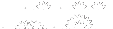
Figure 2: Bosonization’s Feynman diagram series.

III.2 Perturbative results

Before computing the full non-perturbative form of the fermion Green function, let us verify that our bosonized theory, reproduces the perturbative results of Oganesyan, Kivelson and FradkinOganesyan et al. (2001) near the nematic QCP. We shall be interested, therefore, in the integral:

$$\Sigma^{(1)}_{S}({\bf q},\omega)=i\int_{{\mathcal{P}}_{S}}\frac{d^{2}kd\varepsilon}{(2\pi)^{3}}G_{F(S)}^{0}({\bf q-k},\omega-\varepsilon)V_{S,S}(k,\varepsilon)$$ (51)

Here $V_{ss}(k,\varepsilon)$ is the effective interaction mediated by the collective modes, c.f. Eq.(29), Eq.(30) and Eq.(41). The main contribution to the self-energy is due to the overdamped Goldstone modes, as noted in Ref.[Oganesyan et al., 2001]. Thus we take a generic interaction of the form

$$V_{S,S}(k,\varepsilon)=\frac{1/N(0)}{\delta(k)-K_{0}(s)}$$ (52)

noting that $\cos^{2}(2(\theta_{S}-\phi))$, which should appear as a coefficient in the nematic case, only introduces irrelevant contributions to the integral and is therefore left out of this analysis. Here, at the QCP, $\delta(k)=-\kappa k^{2}/2$ but as a check we may characterize the Fermi liquid phase by letting $\delta(k)=\delta$, a constant.

Before computing $\Sigma^{(1)}_{S}({\bf q},\omega)$, we should note that this expression gives the clearest definition of the patch. Given the ultraviolet cutoff $k_{F}-\lambda/2<|{\bf k}|<k_{F}+\lambda/2$, the patch is defined so that in comparison to the original theory

$$\Sigma^{(1)}({\bf k}={\bf k}_{S}+{\bf q},\omega)\approx\Sigma^{(1)}_{S}({\bf q},\omega),\quad{\bf q}\in{\mathcal{P}}_{S}$$ (53)

and therefore the patch width is of order

$$\Lambda\sim\sqrt{k_{F}\lambda}$$ (54)

dictated by the curvature of the Fermi surface alluded to earlier.

Now, to simplify our calculation, let us focus on the fermion lifetime near the Fermi surface:

$$2\Gamma_{S}({\bf q},\omega)=-2\,\mathrm{sign}\,(\omega){\mathcal{I}m}\Sigma_{S}({\bf q},\omega)$$ (55)

This can most easily be expressed in terms of the spectral function, $B_{2}({\bf q},s)$, derived from the imaginary part of $V_{S,S}(q,s)$ as in Eq.(26) and Eq.(41) (after setting the angular factors to 1)

$$2\;\Gamma_{S}({\bf q},\omega)=\\ \int_{-\Lambda/2}^{\Lambda/2}\!\frac{dk_{t}}{2\pi}\int^{q_{n}}_{q_{n}-|\omega|/v_{F}}\!\frac{dk_{n}}{2\pi}\;B_{2}\bigg{(}k,\displaystyle{\frac{\omega-v_{F}(q_{n}-k_{n})}{kv_{F}}}\bigg{)}\\$$ (56)

where $q_{n}$=${\bf v}_{S}\cdot{\bf q}/v_{F}$. Here we note that this integral is dominated by the contribution of the overdamped mode, which enters in $B_{2}^{+}(q,s)$. (The other contributions, associated with the propagating collective modes, only yield regular dependences in the fermion frequency.) Setting $q_{n}\to 0$ and looking at the limit $\omega\to 0$ we obtain

$$\Gamma_{S}(\omega)=\frac{1}{2\pi^{2}}\int_{0}^{\omega/v_{F}}dk_{n}\int_{0}^{\Lambda}dk_{t}B_{2}^{+}(\sqrt{k_{n}^{2}+k_{t}^{2}},\frac{k_{n}}{k_{t}})$$ (57)

using normal and tangential coordinates. From here, we first integrate over the tangential momenta, look at small $q_{n}$ and obtain the long wavelength behavior. We find that in the Fermi Liquid phase ($\delta(k)=\text{const}$)

$$\Gamma_{S}(\omega)\sim\frac{1}{N(0)}\bigg{(}\frac{\omega}{v_{F}}\bigg{)}^{2}|\log\omega/\Lambda v_{F}|$$ (58)

while at the nematic QCP, using $\delta=-\kappa k^{2}/2$:

$$\Gamma_{S}(\omega)\sim\frac{1}{N(0)}\bigg{(}\frac{\omega}{\kappa v_{F}}\bigg{)}^{2/3}$$ (59)

In the Fermi liquid, the energy of the quasiparticle is proportional to $\omega$ and we classify them as long lived. However, at the nematic QCP, one can show via Kramers-Kronig that the real part of the self energy also goes like $|\omega|^{2/3}$. Hence at the nematic QCP, the life time of a quasi particle is not well defined and to try to understand it as a perturbation about a free theory of long lived quasi particles is meaningless.

Thus, the bosonized theory reproduces the results found earlier on perturbatively by Oganesyan and coworkersOganesyan et al. (2001) (see also Ref.[Metzner et al., 2003; Dell’Anna and Metzner, 2005]). It should be noted that the $\omega^{2/3}$ law was also found to appear in the perturbative calculation of the fermion self-energy in a model of holes interacting via a forward scattering $U(1)$ gauge interaction with a similar form to (52) in the context of high temperature superconductorsLee (1989); Altshuler et al. (1995), and in the perturbative treatment of the quantum critical point in a ferromagnetic metal. Chubukov (2005)

III.3 Non-perturbative results

We now return to the non-perturbative bosonized expression for the fermion propagator of Eq.(45), which we will write as

$$G_{F(S)}({\bf x},t)=Z_{S}({\bf x},t)G_{F(S)}^{0}({\bf x},t)$$ (60)

In the Fermi liquid phase and at long distances and low frequencies the factor $Z_{S}$ approaches a constant value, $Z_{S}=Z_{F}<1$, i.e. the quasiparticle residue of the Fermi liquid state. Our goal here is to investigate the behavior of $Z_{S}({\bf x},t)$ near the nematic QCP and in the nematic phase. However, given the complexity of the full analytic expression, in this paper we will consider only on the equal-time, $t=0$, behavior (sometimes called the “one-particle density matrix”) and the equal-position, ${\bf x}=0$, dynamical correlation function, and only at zero temperature. We will discuss its full behavior elsewhere.

III.3.1 The equal-time fermion propagator

As in the perturbative calculation, it is convenient to express $\ln Z$ as an integral over the spectral functions $B_{2}^{\pm}(q,s)$. Once again, at the nematic QCP, the important contribution is due to the overdamped collective mode in $B_{2}^{+}(q,s)$, and we will neglect all other contributions. (This is an approximation which gives the long time behavior accurately. An expression valid for all times also includes the contribution of $B_{2}^{-}(q,s)$.)

Since we have set $t=0$ here, the result is quite simple

$$\ln Z(x_{n},0)=\!\int_{0}^{\lambda/2}\!\frac{dk_{n}}{2\pi}I_{2}(k_{n})\big{(}\cos(k_{n}x_{n})-1\big{)}$$ (61)

where

$$I_{2}(k_{n})=\int_{-\Lambda/2}^{\Lambda/2}\frac{dk_{t}}{2\pi}\int_{0}^{\infty}\frac{d\omega}{2\pi}\frac{B_{2}^{+}(k,\omega/kv_{F})}{\big{(}\omega+v_{F}k_{n}\big{)}^{2}}$$ (62)

We find, both from a numerical computation and from an analytic estimate, that

$$I_{2}(k_{n})=\frac{1}{N(0)v_{F}}\frac{f_{2}\left(k_{n}\sqrt{\kappa}\right)}{\left(k_{n}\sqrt{\kappa}\right)^{4/3}}$$ (63)

where $f_{2}(k_{n}\sqrt{\kappa})$ is a regular function of its argument. From this analysis, we conclude after performing the final Fourier transformation:

$$Z_{S}\left(x_{n},0\right)=C_{P}\exp\left\{-\frac{b}{N(0)v_{F}\sqrt{\kappa}}\left|\frac{x_{n}\!}{\sqrt{\kappa}}\right|^{1/3}\right\}$$ (64)

valid for $|x_{n}|\gg\sqrt{\kappa}$. Here $b=0.0658$ and $C_{P}$ is a constant factor resulting from subdominant terms in $I_{2}(k_{n})$. This sharp decay of $Z_{S}(x_{n},0)$, faster than any power law, introduces a scale (similar to a correlation length arising from a gap in the spectrum) and dominates over the Fermi liquid behavior at low energies. From the above expression, the correlation length is of order $\xi\sim\sqrt{\kappa}(k_{F}\sqrt{\kappa})^{3}$ which is much longer than length of the interactions, $\sqrt{\kappa}$.

Let us also compute the behavior of $Z_{S}$ on the nematic phase by focusing on the effect of the Goldstone modes. Recalling our discussion of the order parameter theory, we replace (52) with

$$V_{S,S}(k,\varepsilon)=\frac{\sin^{2}(2\theta_{S})}{N(0)}\frac{1}{-\kappa k^{2}/2+i|s|\sin^{2}(2\phi)}$$ (65)

which is the contribution from the Goldstone mode ($K_{0}(s)\approx-i|s|$). In the limit, $k_{n}\to 0$, that is on the Fermi surface, $\phi\to\theta_{S}+\pi/2$ and therefore, we simply have

$$V_{S,S}(k,\varepsilon)=\frac{1}{N(0)}\left(-\frac{\kappa k^{2}}{\sin^{2}(2\theta_{S})}-K_{0}(s)\right)^{-1}$$ (66)

so that the difference between this and the symmetric side is simply that $\kappa\to\kappa/\sin^{2}(2\theta_{S})$. Hence, we may directly write down $Z_{S}$:

$$Z_{S}\left(x_{n},0\right)=C_{P(S)}\exp\left\{-\frac{b\left|\sin\left(2\theta_{S}\right)\right|^{4/3}}{N(0)v_{F}\sqrt{\kappa}}\left|\frac{x_{n}\!}{\sqrt{\kappa}}\right|^{1/3}\right\}$$ (67)

where $b$ is the same constant of Eq. (64). In Eq.(67) we have not included the subdominant contributions which become the leading terms along the symmetry-dictated directions, the “nematic axes”, along which the angular factor vanishes. Along the nematic axes the behavior of the equal-time correlation function has a more Fermi liquid like long distance behavior as shown by Oganesyan et. al., but due to the introduction of patchs, we cannot accurately capture this behavior here.

Thus, we see that on the broken symmetry side, we have special points at $\theta_{S}=n\pi/2$ where the Goldstone mode weakens and subdominant behavior takes over. At these points, $Z_{S}=C_{P(S)}=Z_{F}<1$ and the quasiparticles become long lived. It is interesting to note that the angular dependence shown here with a power of $4/3$ is similar to that of the perturbative calculation using the same transformation of $\kappa\to\kappa/\sin^{2}(2\theta_{S})$ on Eq. (59) and it agrees with the results of Ref.[Oganesyan et al., 2001].

III.3.2 The fermion residue

One simple calculation we can do with the above result for $Z_{S}(x_{n},0)$ is the fermion residue following MigdalMigdal (1990).

$$Z_{q} =n({\bf k}_{F}-{\bf q})-n({\bf k}_{F}+{\bf q})$$ (68)

$$=\int\frac{d\omega}{2\pi}\bigg{(}G_{F}({\bf k}_{F}-{\bf q},\omega)-G_{F}({\bf k}_{F}+{\bf q})\bigg{)}e^{i\epsilon\omega}$$ (69)

where the exponential factor tells us to close the contour in the upper half plane. This expression may be written in terms of the real space, real time fermion Green function, at time $t=-\epsilon$. Inserting our expression for $G_{F}$ within Bosonization and neglecting interpatch scattering (which should produce analytic in $q/\Lambda$ contributions here), we obtain:

$$Z_{q_{n}}=\frac{2}{\pi}\int_{0}^{\infty}dx_{n}\frac{\sin q_{n}x_{n}}{x_{n}}Z_{S}(x_{n},0)$$ (70)

In the Fermi liquid phase, we find $Z_{S}(x_{n},0)=Z<1$ in the long distance limit and this leads directly to $Z_{q_{n}}=Z$ when $q_{n}\to 0$ as expected.

At the nematic QCP and into the nematic phase away from the nodal points discussed earlier, $Z_{S}(x_{n},0)$ is short ranged and we may expand to leading order in $q_{n}$ and obtain

$$Z_{q_{n}}\approx\frac{12}{\pi}q_{n}\xi$$ (71)

with the correlation length $\xi=\sqrt{\kappa}(\sqrt{\kappa}k_{F}/2\pi b)^{3}$. Thus the fermion residue vanishes linearly similar to how it would in a Fermi liquid at finite temperature where temperature makes the correlations short ranged. It should be noted, however, that because $Z_{s}(x_{n},0)$ decays slower then $e^{-\alpha x_{n}}$ in the long distance limit, this series expansion that we have used is poorly defined at higher order with the coefficient of $q_{n}^{2j+1}$ growing so rapidly that the Taylor expansion has zero radius of convergence in the complex-$q_{n}$ plane. Thus $Z_{q_{n}}$ is not analytic in $q_{n}$ and the Fermi surface may still be defined as a singular point in $n({\bf k})$. The same behavior occurs in the nematic phase for generic momenta, except along the directions of the nematic principal axes where a finite residue is obtained.

III.3.3 The fermion auto-correlation function

This case turns out to be more complicated than the equal-time expression and we present a full analysis in Appendix D. By a simple integration-by-parts, we found that the double pole of Eq. (62) may be reduced to a single pole and that the integrals involved were less singular by a full power (diverging like $1/k_{n}^{1/3}$ unlike Eq. (63)) but with logarithmic corrections. From that analysis, we found the general form of $Z_{S}$ to be

$$Z_{S}(0,t)=C_{P}\exp\left\{-A(1\!-\!i\sqrt{3})\frac{\ln\left(v_{F}t/\sqrt{\kappa}\right)}{\left(v_{F}t/\sqrt{\kappa}\right)^{2/3}}\right\}$$ (72)

In contrast with our result for the equal-time correlation function, Eq.(72) approaches a constant at long times. However, it decays to that constant much more slowly than in a Fermi liquid where we would expect the exponent $2/3$ to become $2$. As a result, the non-perturbative effects are here less important and, consequently, this time-dependence appears to exhibit the same power-law behavior as the life time calculated perturbatively in Sec. III.2.

The coefficient of the exponential was found to be    $A\propto 1/(k_{F}\lambda\kappa)$ and deserves some attention. In a Fermi liquid, we would find $A\propto\lambda/k_{F}\ll 1$ and the time dependence would present a small correction from the Fermi-liquid behavior. However, $A$ need not be small if $1/\kappa\gg k_{F}\lambda\sim\Lambda^{2}$, where $\Lambda$ is the patch width (c. f. Eq. (54)). Due to the emergence of $\Lambda$ here, this limit occurs precisely where the Fermi-surface curvature begins to matter, and where the interaction length scale is still quite small ($k_{F}^{-1}\ll\sqrt{\kappa}\ll\Lambda^{-1}$).

In the nematic phase, again letting $\kappa\to\kappa/\sin^{2}2\theta_{S}$, we find

$$Z_{S}(0,t)=\\ C_{P(S)}\exp\left\{-A(1\!-\!i\sqrt{3})\left|\sin 2\theta_{S}\right|^{4/3}\frac{\ln\left(\frac{v_{F}t}{\sqrt{\kappa}}|\sin 2\theta_{S}|\right)}{\left(v_{F}t/\sqrt{\kappa}\right)^{2/3}}\right\}$$ (73)

so that the angular dependence is similar to that of the equal-time behavior.

III.3.4 The one-particle density of states

We close this section with an application of these results to the calculation of the one-particle density of states (DOS) in both the Fermi liquid and the nematic phases, and at the nematic (Pomeranchuk) quantum critical point.

The one-particle DOS is defined by the standard expression

$$N^{*}(\omega)=-\,\mathrm{sign}\,(\omega)\;\frac{1}{\pi}\textrm{ Im}\;G_{F}(x,x;\omega)$$ (74)

In Fermi liquid phase, using $Z_{S}(0,t)=C_{F}$, a constant dependent upon the Fermi liquid parameters that goes to 1 for the non-interacting case, as expected we find

$$G_{F}(x,x,\omega) =\sum_{S}\frac{1}{N}C_{F}\int dtG^{0}_{F(S)}(0,t)e^{i\omega t}$$

$$=C_{F}\int dt\frac{N(0)v_{F}}{-v_{F}t+ia\,\mathrm{sign}\,(t)}e^{i\omega t}$$

$$=-i\pi\,\mathrm{sign}\,(\omega)C_{F}N(0)$$ (75)

so that here, $N^{*}(\omega)=C_{F}N(0)$ as expected. Note: $C_{F}$ is not the fermion residue and may be greater than one.

At the nematic QCP, we have instead

$$G_{F}(x,x,\omega)=\sum_{S}\frac{1}{N}\int_{-\infty}^{\infty}dt\;C_{P}\;e^{i\omega t}\exp\left\{-A(1\!-\!i\sqrt{3})\frac{\ln\left(v_{F}t/\sqrt{\kappa}\right)}{\left(v_{F}t/\sqrt{\kappa}\right)^{2/3}}\right\}G^{0}_{F(S)}(0,t)$$ (76)

so that $N^{*}(\omega)=C_{P}N(0)I(\bar{\omega})$ with

$$I(\omega)=\frac{2}{\pi}{\mathcal{R}e}\int_{0}^{\infty}\frac{du}{u}\sin\left(\bar{\omega}u\right)\exp\left\{-A(1\!-\!i\sqrt{3})\frac{\ln u}{u^{2/3}}\right\}\\$$ (77)

with $\bar{\omega}=\sqrt{\kappa}\omega/v_{F}$, valid for $\omega\ll v_{F}\min\{\kappa^{-1/2},\lambda\}$. Notice that we have used throughout these expressions only the long time limit of the exponential factor. At shorter times the behavior of the exponential should be dominated by high energy effects which are insensitive to whether the system is in a Fermi liquid, a quantum critical point or in a nematic phase. Thus, the time integrals have an implicit short distance cutoff (which we have denoted by “$0$”). In any event, we are only interested in the low frequency behavior which is dominated by the long time part of the integration range.

By inspection we see that the exponential factor approaches unity (quite rapidly) for large $u\gg 1$. Thus, the main effect of this factor is a correction to $I(\omega)$ away from its value at zero frequency, i.e., $I(0)=1$. The leading finite frequency behavior, as $\omega\to 0$, is obtained by expanding the exponential factor in Eq.(77):

$$I(\omega) =1-\frac{2A}{\pi}\int_{0}^{\infty}\frac{du}{u}\frac{\sin\bar{\omega}u}{u^{2/3}}\ln u+\ldots$$

$$=1+A\;\frac{3\sqrt{3}}{2\pi}\Gamma(1/3)\left(\frac{\sqrt{\kappa}\omega}{v_{F}}\right)^{2/3}\;\ln\left(\frac{\sqrt{\kappa}\omega}{v_{F}}\right)+\ldots$$

where the last line is accurate for $\sqrt{\kappa}\omega/v_{F}\ll 0.1$. The ellipsis in Eq.(LABEL:eq:Iomega) represents subdominant contributions at low frequencies, which vanish faster than $\omega^{2/3}\ln\omega$ as $\omega\to 0$. As a result, the $\omega^{2/3}$ behavior of the inverse life time $\Gamma(\omega)$ calculated perturbatively, appears here as a cusp in the DOS (with a logarithmic correction). Unlike the lifetime, though, here $A$ depends on the product of the patch width cutoff $\sqrt{k_{F}\lambda}\sim\Lambda$ and $\sqrt{\kappa}$ while $\Gamma(\omega)$ depends only on the product of $k_{F}$ and $\sqrt{\kappa}$.

Thus we find that the low frequency one-particle density of states has the form

$$N^{*}(\omega)=N^{*}(0)+B\;\omega^{2/3}\ln\omega+\ldots$$ (79)

where $N^{*}(0)=C_{P}N(0)>N(0)$, since we found the constant $C_{P}>1$ (see Eq.(142)), and $B=AC_{P}N(0)\frac{3\sqrt{3}}{2\pi}\Gamma(1/3)$ (see Eq.(143)). Hence, the zero frequency value of the density of states is larger than the Fermi liquid value. As the frequency increases, the one-particle density of states decreases from its zero frequency value according to the $\omega^{2/3}\ln\omega$ correction term. This is a cusp singularity at $\omega=0$. It is important to stress that we obtained these expressions upon expanding the exponential factor in the auto-correlation function. This is consistent since this factor asymptotically (and rather rapidly) approaches $1$ at long times. This also implies that, in this regime, our results should be consistent with the behavior of the fermion Green function found in perturbation theory around Hartree-Fock/RPAOganesyan et al. (2001); Metzner et al. (2003); Dell’Anna and Metzner (2005); Chubukov (2005).

In the nematic phase, an angular average of Eq. (73) enters our expression for $N^{*}(\omega)$. In the long time limit, when the argument of the exponential is much less than one, we expect that for low frequencies

$$A\to\left\langle\big{|}\sin 2\theta_{S}\big{|}^{4/3}\right\rangle A\approx 0.58A$$ (80)

Hence, in the nematic phase, the Goldstone modes continue the critical behavior of this function in only a mildly weaker form.

In summary, in this section we used bosonization to compute the non-perturbative behavior of the fermion propagator using the bosonized form of the fermion operator. We first checked that the non-Fermi liquid behavior of the nematic QCP and in the nematic phase, which were obtained earlier using conventional diagrammatic (perturbative) methods,Oganesyan et al. (2001); Metzner et al. (2003) is recovered here upon expanding the bosonized expression to leading order in $V_{SS}$, i.e. a single boson exchange. However, upon a closer examination of the full bosonized result we found that the equal-time fermion correlation function has a much more singular behavior that could have been predicted in perturbation theory. In contrast, the fermion auto-correlation function (and hence the one -particle density of states) is seemingly consistent with the perturbative analysis of the quantum critical behavior.

We note here that ChubukovChubukov (2005), has analyzed the quantum critical behavior of ferromagnetic Fermi liquids and claims that the $\omega^{2/3}$ behavior, found at lowest order, persists to all orders in perturbation theory. The results of this section for the fermion auto-correlation function appear to agree with those of Chubukov and coworkers. However our results for the equal-time fermion correlator apparently disagree with these results. Clearly, a more detailed analysis of the bosonized expression for this propagator is warranted. We will discuss this problem in a separate publication.

IV Conclusion

In this paper, we have utilized the method of high dimensional bosonization to study non-perturbatively the quantum phase transition from a Landau Fermi liquid state to a nematic phase, a nematic (Pomeranchuk) instability. For this purpose, we have constructed an order parameter theory from the boson theory by integrating out non-critical modes and verified that this boson theory is equivalent to RPA. We then turned to studying the bosonization form of the fermion propagator and found its diagrammatic expansion proving the correctness and clarifying the arguments leading up to that expression. This diagrammatic expansion keeps all diagrams up to the simple bubble in the spirit of RPA as applied to the density-density propagator and shows, in specific, that bosonization goes beyond the self-consistent Born approximation to include vertex corrections. We then found explicitly that bosonization reproduces the results of Hartree-Fock with an RPA interaction by showing that the lifetime computed in this limit also has an $|\omega|^{2/3}$ dependence as originally found for the case of the nematic QCP by Oganesyan and coworkers Oganesyan et al. (2001).

Lastly, we calculated the fermion propagator non-perturbatively and found the dramatic effect of the overdamped critical mode that induces short ranged spatial correlations that decay nearly exponentially $\frac{1}{|x|}e^{-{\rm const.}\;|x|^{1/3}}$, while the auto-correlation function exhibits a milder non-Fermi liquid behavior of the form $\frac{1}{|t|}\;\exp(-{\rm const}.\;|t|^{-{2/3}})$. From this short ranged behavior of the equal time Green function, we verify that the fermion residue vanishes at the critical point and into the nematic phase except at four special points. We also calculated the one-particle (fermion) density of states $N^{*}(\omega)$. We found the low frequency behavior $N^{*}(\omega)=N^{*}(0)+B\;\omega^{2/3}\ln\omega$ (with $N^{*}(0)>N(0)$) both at the quantum critical point and into the nematic phase. Thus, the fermion propagator exhibits unexpected behaviors which could not have been anticipated by the existing perturbative resultsOganesyan et al. (2001); Metzner et al. (2003); Vekhter and Chubukov (2004); Chubukov (2005); Nilsson and Castro Neto (2005). In a separate publication we will present a more detailed analysis of the fermion spectral function in both phases and at finite temperature.

Two recent papers, one by Yang Yang (2005) and another by Nilsson and Castro NetoNilsson and Castro Neto (2005), also study Pomeranchuk nematic instabilities in two-dimensional Fermi systems. Yang also derives an order parameter theory within high dimensional bosonization. However, contrary to our results, concludes that the critical mode has $z=2$ and is undamped. While we agree that a $z=2$ propagating mode does exist at the critical point, we find that the spectral function is completely dominated by the overdamped $z=3$ mode. This effect is due to Landau damping, a consequence of the curvature of the Fermi surface, and dominates the low energy behavior of the theory at the critical point. The reason for this disagreement is that in Ref.[Yang, 2005] the effects of Landau damping are ignored. We find that these effects are crucial.

On the other hand, Nilsson and Castro NetoNilsson and Castro Neto (2005) approach the nematic quantum phase transition within the more traditional methods found in the Fermi liquid theory literature. They first find an order parameter theory by constructing a path integral, whose classical equations of motion give the collisionless Boltzmann equation as in high dimensional bosonization, and integrating out the non-critical modes. Their results, however, agree with ours in all essential details, including the existence of a $z=3$ mode. They then calculate the fermion lifetime using the Bethe-Salpeter equations and Fermi’s Golden rule finding that $\tau^{-1}\propto\epsilon^{2/3}$, as in (59), and agree with us, in the perturbative regime, in concluding that this represents both a breakdown of Fermi liquid theory and perturbation theory.

Appendix A Summary of Bosonization in $D$-dimensional Fermi Systems

Consider the Fermi liquid theory of spinless fermions interacting via a short but perhaps finite range forward scattering interaction living in a translationally invariant D-dimensional world. This is a low energy theory and as such, following Landau we shall linearize the energy dispersion near the Fermi surface, though corrections to this may be considered when necessary. To this end, let us build a construction in which we linearize within $N$ equally sized patches approximating the Fermi surface. For this construction to be reasonable, our end result should be relatively insensitive to the details belonging to this partitioning. Keep in mind, however, that a remarkable property of Fermi liquids is that they only require a few of the lowest angular momentum Fermi liquid parameters to understand a wide range of phenomena.

The number of patches, $N$, approximating the Fermi surface will naturally be inversely proportional to its curvature. As such, if the density, $n\to\infty$ then $N\to\infty$ and the construction becomes exact. An exact solution to leading order in $N$ of this linearized theory is therefore equivalent to the asymptotic low energy limit as dictated by the renormalization group. More specifically, the number of patches $N$ and the patch width $\Lambda\sim\sqrt{k_{F}\lambda}$, where $\lambda$ is the energy cutoff, must be related by the condition $2\pi k_{F}=N\Lambda$, required for the Fermi system to a have a finite density of states and curvature (see below). Consequently, the number of patches $N$ must scale as $N\sim 2\pi\sqrt{k_{F}/\lambda}$. Clearly $N\to\infty$ in the infrared limit $\lambda\to 0$. Many of the results of this paper can be understood in light of this basic reasoning.

Under our construction, the fermion annihilation operator becomes:

$$\begin{split}\hat{c}({\bf x})&=\sum_{\bf k}\hat{c}_{\bf k}\frac{e^{i{\bf k}\cdot{\bf x}}}{\sqrt{L^{D}}}\\ &=\sum_{S}\sum_{{\bf q}\in{\mathcal{P}}_{S}}\hat{c}_{{\bf k}_{S}+{\bf q}}\frac{e^{i({\bf k}_{S}+{\bf q})\cdot{\bf x}}}{\sqrt{L^{D}}}\\ &=\sum_{S}\hat{c}_{S}({\bf x})\frac{e^{i{\bf k}_{S}\cdot{\bf x}}}{\sqrt{N}}\end{split}$$ (81)

where $S$ labels the patch, ${\mathcal{P}}_{S}$ is the volume in ${\bf k}$-space around the point ${\bf k}_{S}$ and the new fermion operators, $\psi_{S}({\bf x})$, obey the canonical commutation relations

$$\big{\{}c_{S}({\bf x}),c^{\dagger}_{T}({\bf x^{\prime}})\big{\}}=\delta_{S,T}\delta^{D}({\bf x-x^{\prime}})$$ (82)

It is also important to note the Fourier transform normalizations within the construction:

$$\begin{split}&\delta^{D}({\bf x-x^{\prime}})=\delta^{D-1}_{t}({\bf x_{t}-x_{t}^{\prime}})\delta(x_{n}-x_{n}^{\prime})\\ &=\bigg{(}N\!\sum_{|{\bf q_{t}}|<\frac{\Lambda}{2}}\frac{e^{i{\bf q_{t}}\cdot({\bf x_{t}-x_{t}^{\prime}})}}{L^{(D-1)}}\bigg{)}\bigg{(}\sum_{|{\bf q_{n}}|<\frac{\lambda}{2}}\frac{e^{iq_{n}(x_{n}-x_{n}^{\prime})}}{L}\bigg{)}\end{split}$$ (83)

where we have introduced $\Lambda$ to characterize the tangential width of the patch ($N\Lambda$ is the area of the Fermi surface) and $\lambda$ as an ultraviolet cutoff about the Fermi surface.

Now, in terms of our fermion operators, the linearized Hamiltonian is

$$:\!\hat{H}\!:\ =\sum_{S}\int d^{\bf x}\ \bigg{(}{\mathcal{H}}^{0}_{S}({\bf x})+{\mathcal{H}}^{\text{Int}}_{S}({\bf x})\bigg{)}$$ (84)

where the free Hamiltonian density is

$${\mathcal{H}}_{0}({\bf x})=\frac{\hbar}{2i}{\bf v}_{S}\cdot\bigg{(}:\!\big{(}{\bf\nabla}\hat{c}^{\dagger}_{S}({\bf x})\big{)}\hat{c}_{S}({\bf x})-\hat{c}^{\dagger}_{S}({\bf x}){\bf\nabla}\hat{c}_{S}({\bf x})\!:\bigg{)}$$ (85)

and the forward scattering interactions are described by

$${\mathcal{H}}^{\text{Int}}_{S}({\bf x})=\sum_{T}\int d{\bf x}^{\prime}F_{S-T}({\bf x-x^{\prime}})\delta\hat{n}_{S}({\bf x})\delta\hat{n}_{T}({\bf x^{\prime}})$$ (86)

Here, the density fluctuations are defined by

$$\delta\hat{n}_{S}({\bf x})\equiv\ :\!\hat{n}_{S}({\bf x})\!:\ =\ :\!\hat{c}_{S}^{\dagger}({\bf x})\hat{c}_{S}({\bf x})\!:$$ (87)

and throughout this description we have been using the usual normal ordering procedure for any operator ${\mathcal{O}}$:

$$:\!{\mathcal{O}}\!:\big{|}G\rangle=0\to{\mathcal{O}}\ =\ :\!{\mathcal{O}}\!:-\langle G\big{|}{\mathcal{O}}\big{|}G\rangle$$ (88)

where we take the filled Fermi sea as our ground state:

$$\big{|}G\rangle=\prod_{S}\prod_{\{{\bf q}\in{\mathcal{P}}_{S}|{\bf v}_{S}\cdot{\bf q}<0\}}\hat{c}_{{\bf q},S}^{\dagger}\big{|}0\rangle$$ (89)

It was shown by HaldaneHaldane (1992, 1994), Castro Neto and FradkinCastro Neto and Fradkin (1994a, b); Castro Neto and Fradkin (1995) and Houghton and MarstonHoughton and Marston (1993); Houghton et al. (2000) that this Hamiltonian can be entirely described in terms of the electron density operators, $\delta\hat{n}_{S}({\bf x})$ in the high density limit and it is quadratic in these operators. A fermion operator may then be constructed following well known 1D bosonization techniques and so the theory can be solved exactly. (This represented a major step forward since the introduction of RPA by Bohm and PinesPines and Nozières (1966,1989).) Here we shall outline the proof of this solution, but with the traditional approach of point-splitting regularization, commonly used in the one-dimensional case (see for exampleAffleck (1986)).

The expectation value of the density operator $\hat{n}_{S}({\bf x})$ in the ground state of the Fermi sea is clearly divergent if we send the density of fermions to infinity. As a result, in the high density limit we are interested in, it is poorly defined. To control this divergence, we introduce the point-split operator:

$$\begin{split}\hat{n}_{S}^{\epsilon}({\bf x})&\equiv\hat{c}_{S}^{\dagger}({\bf x+\epsilon/2})\hat{c}_{S}({\bf x-\epsilon/2})\\ &=\ :\!\hat{n}_{S}^{\epsilon}({\bf x})\!:-\langle G\big{|}\hat{n}_{S}^{\epsilon}({\bf x})\big{|}G\rangle\end{split}$$ (90)

Here, by short-distance it is meant a length scale short compared with the separation of all operators of interest but long compared with physical short length scales, i.e. It should be noted that physically point-splitting can be thought of as a means of $|{\bf x}|\gg|\epsilon|\gg\lambda^{-1}$.

The divergent part may be computed explicitly:

$$\begin{split}\langle G\big{|}\hat{n}_{S}^{\epsilon}({\bf x})\big{|}G\rangle&=\frac{N}{L^{D}}\sum_{{\bf q_{t}}}\sum_{q_{n}<0}e^{-i{\bf q}\cdot{\bf\epsilon}}\\ &=\delta^{D-1}_{t}({\bf\epsilon_{t}})\int_{-\infty}^{0}\frac{dq_{n}}{2\pi}e^{-iq_{n}\epsilon_{n}+q_{n}/\lambda}\\ &=\frac{i\delta^{D-1}_{t}({\bf\epsilon_{t}})}{2\pi(\epsilon_{n}+i\lambda^{-1})}\end{split}$$ (91)

where we have implemented the ultraviolet cutoff, $\lambda$, as a soft cutoff $e^{-|q_{n}|/\lambda}$. This is a highly anisotropic expression in ${\bf\epsilon}$. It vanishes if we first send $\epsilon_{n}\to 0$, looking along a tangential direction (${|\bf\epsilon}_{t}|\gg\Lambda^{-1}\to 0$) but diverges if we first send $\epsilon_{t}\to 0$ looking along $\epsilon_{n}\gg\lambda^{-1}\to 0$. Therefore, to capture the basic physics of the density operator we must choose the latter limit as the definition of the point split operator. Keeping in mind that $\delta_{t}(0)=A_{F}/(2\pi)^{D-1}=2\pi\hbar v_{F}N(0)$, where $A_{F}$ is the $(D-1)$-dimensional Fermi surface area and $N(0)$ is the density of states at the Fermi surface, we obtain

$$\hat{n}_{S}^{\epsilon_{n}}({\bf x})=-\frac{iN(0)\hbar v_{F}}{\epsilon_{n}}+\delta\hat{n}_{S}({\bf x})+\frac{i\epsilon_{n}}{\hbar v_{F}}{\mathcal{H}}_{S}^{0}({\bf x})+\ldots$$ (92)

to leading order in $\epsilon_{n}\gg\lambda^{-1}$ and where we kept the expansion of $:\!\hat{n}_{S}^{\epsilon_{n}}({\bf x})\!:$ to first order noticing the useful emergence of the free Hamiltonian density operator.

Now that we have a controlled definition of the density operator, we proceed with computing its commutator:

$$\big{[}\hat{n}^{\epsilon_{n}}_{S}({\bf x}),\hat{n}^{\epsilon_{n}^{\prime}}_{T}({\bf x^{\prime}})\big{]}=\frac{iN(0)\hbar v_{F}}{\epsilon_{n}+\epsilon_{n}^{\prime}}\delta_{S,T}\delta_{t}^{D-1}({\bf x_{t}-x_{t}^{\prime}})\\ \times\bigg{(}\delta\big{(}x_{n}-x_{n}^{\prime}-(\epsilon_{n}+\epsilon_{n}^{\prime})/2\big{)}-\delta\big{(}x_{n}-x_{n}^{\prime}+(\epsilon_{n}+\epsilon_{n}^{\prime})/2\big{)}\bigg{)}$$ (93)

Expanding both sides of this equation in powers of $\epsilon_{n}$ and equating like powers gives us the following result

$$\big{[}\delta\hat{n}_{S}({\bf x}),\delta\hat{n}_{T}({\bf x^{\prime}})\big{]} =-i\hbar N(0)\delta_{S,T}{\bf v}_{S}\cdot\nabla\delta^{D}({\bf x-x^{\prime}})$$ (94)

$$\big{[}\delta\hat{n}_{S}({\bf x}),{\mathcal{H}}_{T}^{0}({\bf x^{\prime}})\big{]} =-i\hbar{\bf v}_{S}\cdot\nabla\delta\hat{n}_{S}({\bf x})\delta^{D}({\bf x-x^{\prime}})$$ (95)

Using these commutators, we may compute the equation of motion for the Heisenberg operator $\delta\hat{n}_{S}({\bf x},t)$:

$$\partial_{t}\delta\hat{n}_{S}({\bf x},t)+{\bf v}_{S}\cdot\nabla\delta\hat{n}_{S}({\bf x},t)+\\ {\bf v}_{S}\cdot\nabla\sum_{T}\int d{\bf x}^{\prime}F_{S-T}({\bf x-x^{\prime}})\delta\hat{n}_{T}({\bf x^{\prime}},t)=0$$ (96)

where $F_{S-T}=N(0)f_{S-T}$. This is the linearized collisionless Boltzmann equation in operator form found by Castro Neto and Fradkin in the context of a coherent state formalismCastro Neto and Fradkin (1994a). We also notice through this derivation that we may let

$${\mathcal{H}}_{S}^{0}({\bf x})=\frac{1}{2N(0)}\delta\hat{n}_{S}^{2}({\bf x})$$ (97)

and obtain exactly the same answer. Hence, the Hamiltonian may be expressed entirely in terms of the density operator $\delta\hat{n}_{S}({\bf x})$.

A natural consequence of (94) is that the density operator may be expressed in terms of a chiral boson field:

$$\delta\hat{n}_{S}({\bf x})=N(0){\bf v}_{S}\cdot\nabla\hat{\varphi}_{S}({\bf x})$$ (98)

with a canonically conjugate momentum

$$\hat{\pi}_{S}({\bf x})=-N(0){\bf v}_{S}\cdot\nabla\hat{\varphi}_{S}({\bf x})$$ (99)

These chiral bosons are a direct extension of the right / left chiral bosons in the context of 1D bosonization. Following this extension then, we may express the fermion operator as a vertex operator

$$\hat{\psi}_{S}({\bf x})=\eta_{S}({\bf x}_{t})\sqrt{N(0)v_{F}\lambda}:\!e^{-i\hat{\varphi}_{S}({\bf x})/\hbar}\!:$$ (100)

where $\eta_{S}({\bf x}_{t})$ is a set of Klein factors responsible for ensuring that $\hat{\psi}_{S}({\bf x})$ obey the proper anti-commutation relations within the patch and on different patches. The relation between this fermion operator and the original $\hat{c}_{S}(x)$-operators will be made precise in Section III.1 via direct comparison of the perturbation series in $F_{S-T}({\bf x-x^{\prime}})$ obtained in the bosonized theory. $\hat{\psi}_{S}({\bf x})$, therefore, is equivalent to $\hat{c}_{S}({\bf x})$ in the free case and in the interacting case, it is this operator projected onto the high-density subspace. Hence, this is an effective low energy theory of a dense Fermi system and $\hat{\psi}^{\dagger}_{S}({\bf x})$ can be viewed as actually creating Landau quasiparticles in the Fermi liquid phase.

The canonical structure of the bosonized theory also allows us to directly write down a path integral formulation of the problem, including interactions described by a set of Landau parameters (for a derivation using coherent states, see Ref.[Castro Neto and Fradkin, 1994a]). The action for the bosonized theory has the general form

$$S=\frac{N(0)}{2}\sum_{S}\!\int d^{2}xdt\bigg{[}-\partial_{t}\varphi_{S}{\bf v}_{S}\cdot\nabla\varphi_{S}-\big{(}{\bf v}_{S}\cdot\nabla\varphi_{S}\big{)}^{2}\bigg{]}+\frac{N(0)}{2}\sum_{S,T}\int d^{2}xd^{2}x^{\prime}dtF_{S-T}({\bf x-x^{\prime}}){\bf v}_{S}\cdot\nabla\varphi_{S}({\bf x}){\bf v}_{T}\cdot\nabla\varphi_{T}({\bf x^{\prime}})$$ (101)

This action is a quadratic form in the Bose fields. Here we have not included higher order terms (such as those discussed in the body of the paper, in the context of the nematic instability). Such terms are generally present due to non-linearities in the fermion dispersion relation, as well as many-body effective interactions.Barci and Oxman (2003) We have also not included “vertex operators” such as those associated with pairing (BCS) interactions.Castro Neto and Fradkin (1994a); Houghton et al. (2000) We shall find it more convenient to work within this path-integral formulation when constructing a theory of the nematic quantum critical point.

Before leaving our discussion of high dimensional bosonization, we should make a final comment on its validity. As discussed in the main body of the paper, the boson theory here completely recovers the random phase approximation (RPA) in the long wavelength limit. This should not be surprising since, in the asymptotic low energy limit, both RPA and bosonization saturate the f-sum rule and are (formally) exact. This is a well known established property of bosonization, extensively discussed in the literature since the 1970’s.

Appendix B Analysis of $V_{2}^{+}$ and $V_{2}^{-}$

Here we present the partial fraction expansion of the effective interactions $V_{2}^{+}$ and $V_{2}^{-}$ and their behavior near quantum criticality.

B.1 Partial fraction expansion of $V_{2}^{+}(q,s)$

In terms of the function $K_{0}(s)$ we may write $V_{2}^{+}$ as

$$\begin{split}V^{+}_{2}(q,s)&=\frac{1}{N(0)}\Bigg{[}\delta_{2}(q)-K_{0}(s)\bigg{(}1+\bigg{(}\tfrac{1-K_{0}(s)}{1+K_{0}(s)}\bigg{)}^{2}\bigg{)}\Bigg{]}^{-1}\\ &=\frac{1}{2N(0)}\bigg{[}\frac{(1+x)^{2}}{x^{3}-\frac{\delta_{2}}{2}x^{2}+(1-\delta_{2}(q))x-\frac{\delta_{2}(q)}{2}}\bigg{]}\end{split}$$ (102)

where $x=K_{0}(s)$. The denominator is thus a cubic polynomial in $K_{0}(s)$ and solving for the poles, $x=\delta_{\beta}^{+}(q)$, we find

$$\delta_{\beta}^{+}(q)=\bigg{\{}\frac{1}{6}\big{(}\delta_{2}(q)+\frac{\delta_{2}(q)^{2}+12\delta_{2}(q)-12}{e^{in\pi/3}h(\delta_{2}(q))}\\ +e^{in\pi/3}h(\delta_{2}(q))\big{)}\bigg{|}n\in\{-1,1,3\}\bigg{\}}$$ (103)

where

$$h(x)=(12\sqrt{12-36x+42x^{2}+3x^{3}}-x(x^{2}+18x+36))^{1/3}$$ (104)

and we assign $\beta=\{a,b,c\}$ to each of these three poles. The partial fraction expansion is

$$V^{+}_{2}(q,s)=\frac{1}{N(0)}\sum_{\beta=a,b,c}\frac{{\mathcal{Z}}^{+}_{\beta}(q)}{\delta^{+}_{\beta}(q)-K_{0}(s)}$$ (105)

with residues

$$\begin{split}{\mathcal{Z}}_{a}^{+}(q)&=\frac{1}{2}\frac{(1+\delta_{a}^{+})^{2}}{(\delta_{a}^{+}-\delta_{b}^{+})(\delta_{a}^{+}-\delta_{c}^{+})}\\ {\mathcal{Z}}_{b}^{+}(q)&=\frac{1}{2}\frac{(1+\delta_{b}^{+})^{2}}{(\delta_{b}^{+}-\delta_{a}^{+})(\delta_{b}^{+}-\delta_{c}^{+})}\\ {\mathcal{Z}}_{c}^{+}(q)&=\frac{1}{2}\frac{(1+\delta_{c}^{+})^{2}}{(\delta_{c}^{+}-\delta_{a}^{+})(\delta_{c}^{+}-\delta_{b}^{+})}\end{split}$$ (106)

For $|\delta_{2}(q)|\ll 1$ these formulas simplify to:

$$\delta_{a}^{+} \approx i, \delta_{b}^{+} \approx-i, \delta_{c}^{+} \approx\delta_{2}/2$$ (107)

$${\mathcal{Z}}_{a}^{+} \approx i/2, {\mathcal{Z}}_{b}^{+} \approx-i/2, {\mathcal{Z}}_{c}^{+} \approx 1/2$$ (108)

as a result we may write near the nematic QCP:

$$V_{2}^{+}(q,s)\approx\frac{1}{2N(0)}\bigg{[}\frac{1}{\frac{\delta_{2}(q)}{2}-K_{0}(s)}-\frac{1/4}{s^{2}-1/2}\bigg{]}$$ (109)

B.2 Partial fraction expansion of $V_{2}^{-}(q,s)$

We may write $V_{2}^{-}(q,s)$ as

$$V^{-}_{2}(q,s)=\frac{1}{N(0)}\bigg{[}\delta_{2}(q)-K_{0}(s)\bigg{(}1-\bigg{(}\tfrac{1-K_{0}(s)}{1+K_{0}(s)}\bigg{)}^{2}\bigg{)}\bigg{]}^{-1}\\ =\frac{1}{(4-\delta_{2}(q))N(0)}\bigg{[}\frac{1}{(1+x)^{2}}{x^{2}-2\frac{\delta_{2}(q)}{4-\delta_{2}}x-\frac{\delta_{2}}{4-\delta_{2}}}\bigg{]}\\$$ (110)

The denominator is simply quadratic and we find poles at $x=\delta_{\beta}^{-}$ with

$$\delta_{a}^{-}(q)=-\frac{\sqrt{\delta_{2}(q)}}{\sqrt{\delta_{2}(q)}+2},\quad\delta_{b}^{-}(q)=-\frac{\sqrt{\delta_{2}(q)}}{\sqrt{\delta_{2}(q)}-2}$$ (111)

Hence, we can now expand in partial fractions to obtain

$$V^{-}_{2}(q,s)=\frac{1}{N(0)}\bigg{(}\frac{{\mathcal{Z}}^{-}_{a}(q)}{\delta^{-}_{a}(q)-K_{0}(s)}+\frac{{\mathcal{Z}}^{-}_{b}(q)}{\delta^{-}_{b}(q)-K_{0}(s)}\bigg{)}$$ (112)

with residues

$${\mathcal{Z}}_{a}^{-}=\frac{1}{4-\delta_{2}}\bigg{[}\frac{(1+\delta_{a}^{-})^{2}}{\delta_{a}^{-}-\delta_{b}^{-}}\bigg{]},\quad{\mathcal{Z}}_{b}^{-}=\frac{1}{4-\delta_{2}}\bigg{[}\frac{(1+\delta_{b}^{-})^{2}}{\delta_{b}^{-}-\delta_{a}^{-}}\bigg{]}$$ (113)

Again, these formulas simplify for $|\delta_{2}|\ll 1$:

$$\delta_{a}^{-} \approx-\frac{\sqrt{\delta_{2}}}{2}, \delta_{b}^{-} \approx\frac{\sqrt{\delta_{2}}}{2}$$ (114)

$${\mathcal{Z}}_{a}^{-} \approx-\frac{1}{4\sqrt{\delta_{2}}}, {\mathcal{Z}}_{b}^{-} \approx\frac{1}{4\sqrt{\delta_{2}}}$$ (115)

Thus, near the Nematic QCP we can write:

$$V_{2}^{-}(q,s)\approx\frac{1}{4N(0)}\bigg{(}\frac{1}{s^{2}+\frac{\delta_{2}(q)}{4}}\bigg{)}$$ (116)

Appendix C Inclusion of $F_{0}(q)$

Here we calculate $V_{S,T}$ for the case when both $F_{0}$ and $F_{2}$ are present and we let $F_{2}$ approach the Nematic QCP ($F_{2}\to-1$). We shall find, however, that the critical behavior is utterly independent of $F_{0}$! Now, let

$$F_{S-T}(q)=\frac{2}{N}\bigg{(}F_{0}+F_{2}(q)\cos\big{(}2(\theta_{S}-\theta_{T})\big{)}\bigg{)}$$ (117)

Returning to the $\sigma_{\ell}^{\alpha}$-theory, whose correlators are the RPA interaction $V_{S,T}$, we find in this case

$$S_{\sigma}=-\frac{1}{2}\int\frac{d^{2}qd\omega}{(2\pi)^{2}}\bigg{[}{\bf\sigma}^{+}({\bf q},\omega)\cdot\big{(}{\bf V}^{+}\big{)}^{-1}\cdot{\bf\sigma}^{+}(-{\bf q}.-\omega)\\ +V^{-}_{2}\big{|}\sigma^{-}_{2}\big{|}^{2}\bigg{]}$$ (118)

where ${\bf\sigma}^{+}=\big{(}\sigma_{0}^{+},\sigma_{2}^{+}\big{)}$ and

$$\big{(}{\bf V}^{+}\big{)}^{-1}=\begin{pmatrix}2\big{(}\chi_{0}^{0}-\frac{1}{F_{0}}\big{)}&2\chi_{2}^{0}\\ 2\chi_{2}^{0}&\chi_{0}^{0}+\chi_{4}^{0}-\frac{1}{F_{2}}\end{pmatrix}$$ (119)

As a result, $V^{-}_{2}$ is completely unaffected by the presence of $F_{0}$ due to the fact that there is no $\sigma_{0}^{-}$ field and opposite “signs” decouple.

Again, we may write this expression as a function of $x=K_{0}(s)$ and taking the inverse, we find

$${\bf V}^{+}=\frac{1}{x^{3}+ax^{2}+bx+c}{\bf W}(x)$$ (120)

where

$${\bf W}(x)=\frac{1}{2\delta_{0}+\delta_{2}-4}\times\\ \begin{pmatrix}-x^{3}+\big{(}\delta_{2}/2\big{)}x^{2}-(1-\delta_{2})x+\delta_{2}/2&x(1-x^{2})\\ x(1-x^{2})&\delta_{0}(1+x)^{2}\end{pmatrix}$$ (121)

and

$$a=\frac{(2-\delta_{0})\delta_{2}}{2\delta_{0}\!+\!\delta_{2}\!-\!4},\quad b=\frac{2\delta_{0}+\delta_{2}-2\delta_{0}\delta_{2}}{2\delta_{0}\!+\!\delta_{2}\!-\!4},\quad c=\frac{-\delta_{0}\delta_{2}}{2\delta_{0}\!+\!\delta_{2}\!-\!4}$$ (122)

with $\delta_{0}=1+1/F_{0}$ and $\delta_{2}=1+1/F_{2}$. Again we find that the polynomial is cubic. Hence, the addition of $F_{0}$ only complicates the algebra, but not the general structure of the solution. We therefore continue as in Appendix B.

Solving the cubic equation in (120) leads to an algebraically complicated result. However, it simplifies near the nematic QCP and we find to lowest order in $\delta_{2}$:

$$\delta_{a}^{+}=i\sqrt{\frac{\delta_{0}}{\delta_{0}-2}},\quad\delta_{b}^{+}=-i\sqrt{\frac{\delta_{0}}{\delta_{0}-2}},\quad\delta_{c}^{+}=\delta_{2}/2$$ (123)

which return to our previous result if we let $F_{0}\to 0$ or $\delta_{0}\to\infty$. Notice that, to lowest order $\delta_{c}^{+}$ is independent of $F_{0}$, as it should since the s-wave mode is non-critical and this “pole” precisely represents the critical behavior. Expanding in partial fractions leads to the expression

$${\bf V}=\frac{1}{N(0)}\sum_{\beta=a,b,c}\frac{{\bf Z}_{\beta}^{+}}{\delta_{\beta}-K_{0}(s)}$$ (124)

with residue matrices

$$\begin{split}{\bf Z}_{a}^{+}&=\frac{i}{2}\sqrt{\frac{\delta_{0}}{\delta_{0}-2}}\begin{pmatrix}\frac{1}{\delta_{0}\big{(}\delta_{0}-2\big{)}}&\frac{\delta_{0}-1}{\delta_{0}\big{(}\delta_{0}-2\big{)}}\\ \frac{\delta_{0}-1}{\delta_{0}\big{(}\delta_{0}-2\big{)}}&1+\frac{i}{\sqrt{\delta_{0}\big{(}\delta_{0}-2\big{)}}}\end{pmatrix}\\ {\bf Z}_{b}^{+}&=\frac{-i}{2}\sqrt{\frac{\delta_{0}}{\delta_{0}-2}}\begin{pmatrix}\frac{1}{\delta_{0}\big{(}\delta_{0}-2\big{)}}&\frac{\delta_{0}-1}{\delta_{0}\big{(}\delta_{0}-2\big{)}}\\ \frac{\delta_{0}-1}{\delta_{0}\big{(}\delta_{0}-2\big{)}}&1-\frac{i}{\sqrt{\delta_{0}\big{(}\delta_{0}-2\big{)}}}\end{pmatrix}\\ {\bf Z}_{c}^{+}&=\frac{1}{2}\begin{pmatrix}0&0\\ 0&1\end{pmatrix}\end{split}$$ (125)

which again returns to the previous result if we let $F_{0}\to 0$. Notice that ${\bf Z}_{c}^{+}$ is independent of $F_{0}$ to this order in $\delta_{2}$. Consequently, the critical behavior of the fermions, (64), is unaffected by the inclusion of a non-critical mode such as $F_{0}$.

Appendix D Equal-Position Boson Propagator

	$\lim_{\{\nu,u_{n}\}\to 0^{-}}$	$\lim_{\{\nu,u_{n}\}\to 0^{+}}$
$I_{\nu}(\nu)$	$-0.0053\ln(\nu)/\nu^{1/3}$	$0.0053\ln(\nu)/\nu^{1/3}$
$I^{\prime}_{\nu}(\nu)$	$-0.0018\ln^{2}(\nu)$	$-0.0018\ln^{2}(\nu)$
${I^{\prime}_{\nu}}^{(1)}(\nu)$	$0.0077/\nu^{1/3}$	$-0.0077/\nu^{1/3}$
$I_{u}(u_{n})$	$0.0280/u_{n}^{1/3}$	$0.0140/u_{n}^{1/3}$
$I^{\prime}_{u}(u_{n})$	$0.0052\ln^{2}(u_{n})$	$-0.0052\ln^{2}(u_{n})$

Table 1: Low frequency / long wavelength limit of the required integrals

Here we are interested in the quantity

$$G_{B(S,S)}({\bf 0},t)=G_{B(S,S)}^{0}({\bf 0},t)+\\ i\int\frac{d^{2}kd\varepsilon}{(2\pi)^{3}}G^{0}_{F(S)}(k,\varepsilon)V_{S,S}(k,\varepsilon)G^{0}_{F(S)}(k,\varepsilon)\left(e^{-i\varepsilon t}-1\right)$$ (126)

the equal position part of Eq. (38). In particular, we focus on the second term, labeling it $\ln Z_{S}({\bf 0},t)$. We begin by writing the interaction in terms of its spectral function:

$$V_{S,S}(k,\varepsilon)=\int\frac{d\varepsilon^{\prime}}{2\pi}\frac{B(k,\varepsilon^{\prime})}{\varepsilon-\varepsilon^{\prime}+i\epsilon^{\prime}\,\mathrm{sign}\,\varepsilon^{\prime}}$$ (127)

where

$$B({\bf k},\omega)=B_{2}^{+}(k,\omega)\cos^{2}\big{(}2(\theta_{S}-\phi)\big{)}\\ +B_{2}^{-}(k,\omega)\sin^{2}\big{(}2(\theta_{S}-\phi)\big{)}$$ (128)

and $\phi$ the direction of ${\bf k}$. Note: in the appropriate scaling within a patch, $\phi\to\theta_{S}+\pi/2$ so that the cosine factor scales to $1$ while the sine factor scales to $0$ driving the $B_{2}^{-}(k,\omega)$ contribution irrelevant (this has been checked explicitely).

This allows us to do the $\varepsilon$-integration immediately and rewrite our expression in a more physical form. The result is (after letting $\epsilon^{\prime}\to 0$):

$$\ln Z_{S}({\bf 0},|t|)=\\ \int_{-\Lambda/2}^{\Lambda/2}\frac{dk_{t}}{2\pi}\int_{-\lambda/2}^{\lambda/2}\frac{dk_{n}}{2\pi}\int_{0}^{\infty}\frac{d\varepsilon}{2\pi}B(k,\varepsilon)R_{1}(k_{n},\varepsilon,|t|)+\\ \int_{-\Lambda/2}^{\Lambda/2}\frac{dk_{t}}{2\pi}\int_{0}^{\lambda/2}\frac{dk_{n}}{2\pi}\int_{-\infty}^{\infty}\frac{d\varepsilon}{2\pi}B(k,\varepsilon)R_{2}(k_{n},\varepsilon,|t|)$$ (129)

which we have written directly in terms of the patch coordinates. The residue of the single pole is:

$$R_{1}(k_{n},\varepsilon,|t|) =\frac{e^{-i\varepsilon|t|}-1}{\left(\varepsilon-v_{F}k_{n}+i\epsilon\,\mathrm{sign}\,\varepsilon\right)^{2}}$$ (130)

$$=\frac{1}{v_{F}}\frac{d}{dk_{n}}\left[\frac{e^{-i\varepsilon|t|}-1}{\varepsilon-v_{F}k_{n}+i\epsilon\,\mathrm{sign}\,\varepsilon}\right]$$ (131)

and the residue of the double pole is

$$R_{2}(k_{n},\varepsilon,|t|)=-\frac{1}{v_{F}}\frac{d}{dk_{n}}\left[\frac{e^{-ik_{n}|t|}-1}{\varepsilon-v_{F}k_{n}+i\epsilon\,\mathrm{sign}\,\varepsilon}\right]$$ (132)

so that it is clear that an integration-by-parts removes the double pole all together, leaving us with an integral only over a single pole. One can view this as a cancelation of the double pole’s contribution to the integral and expect the result to be less singular than the equal-time case.

Using the symmetries of the spectral function, we may rewrite Eq. (129) as

$$\ln Z_{S}({\bf 0},|t|)=\int_{-\infty}^{\infty}\frac{dk_{t}}{2\pi}\int_{0}^{\infty}\frac{dk_{n}}{2\pi}\int_{0}^{\infty}\frac{d\varepsilon}{2\pi}B(k,\varepsilon)\times\\ \bigg{[}R_{1}(k_{n},\varepsilon,|t|)+R_{1}(-k_{n},\varepsilon,|t|)+R_{2}(k_{n},\varepsilon,|t|)-R_{2}(k_{n},-\varepsilon,|t|)\bigg{]}\\$$ (133)

Performing the integration by parts, and a quick change of variables allows us to separate the time dependence in terms of the following integrals:

$$\ln Z_{S}({\bf 0},|t|)=\frac{1}{N(0)v_{F}\sqrt{\kappa}}\Bigg{[}-2\int_{0}^{\infty}d\nu\bigg{(}I^{\prime}_{\nu}(-\nu)-\frac{1}{\lambda\sqrt{\kappa}}\big{(}I_{\nu}(-\nu)+{I^{\prime}_{\nu}}^{(1)}(-\nu)\big{)}\bigg{)}+\\ \int_{0}^{\infty}du_{n}\bigg{(}I_{u}^{\prime}(-u_{n})+I_{u}^{\prime}(u_{n})-\frac{1}{\lambda\sqrt{\kappa}}\big{(}I_{u}(-u_{n})+I_{u}(u_{n})+u_{n}I_{u}^{\prime}(-u_{n})+u_{n}I_{u}^{\prime}(u_{n})\big{)}\bigg{)}e^{-iu_{n}|\bar{t}|}\\ +\int_{0}^{\infty}d\nu\bigg{(}I_{\nu}^{\prime}(-\nu)-I_{\nu}^{\prime}(\nu)-\frac{1}{\lambda\sqrt{\kappa}}\big{(}I_{\nu}(-\nu)-I_{\nu}(\nu)+{I^{\prime}_{\nu}}^{(1)}(-\nu)-{I^{\prime}_{\nu}}^{(1)}(\nu)\big{)}\bigg{)}e^{-i\nu|\bar{t}|}\bigg{]}$$ (134)

where we have sent the cutoffs to infinity, keeping the lowest order correction in $\lambda$ (having checked that higher orders are non-singular), and where the various integrals are

$$I_{\nu}(\nu) =\frac{1}{4\pi^{3}}{\mathcal{P}}\int_{0}^{\infty}du_{t}\int_{0}^{\infty}du_{n}\frac{B(u,\nu)}{\nu-u_{n}}$$ (135)

$$I^{\prime}_{\nu}(\nu) =\frac{1}{4\pi^{3}}{\mathcal{P}}\int_{0}^{\infty}du_{t}\int_{0}^{\infty}du_{n}\frac{\frac{d}{du_{n}}B(u,\nu)}{\nu-u_{n}}$$ (136)

$${I^{\prime}_{\nu}}^{(1)}(\nu) =\frac{1}{4\pi^{3}}{\mathcal{P}}\int_{0}^{\infty}du_{t}\int_{0}^{\infty}du_{n}\frac{u_{n}\frac{d}{du_{n}}B(u,\nu)}{\nu-u_{n}}$$ (137)

$$I_{u}(u_{n}) =\frac{1}{4\pi^{3}}{\mathcal{P}}\int_{0}^{\infty}du_{t}\int_{0}^{\infty}d\nu\frac{B(u,\nu)}{\nu-u_{n}}$$ (138)

$$I^{\prime}_{u}(u_{n}) =\frac{1}{4\pi^{3}}{\mathcal{P}}\int_{0}^{\infty}du_{t}\int_{0}^{\infty}d\nu\frac{\frac{d}{du_{n}}B(u,\nu)}{\nu-u_{n}}$$ (139)

In this latest form of $\ln Z_{S}$, we have defined ${\bf u}={\bf k}\sqrt{\kappa}$, $\nu=\varepsilon\sqrt{\kappa}/v_{F}$, $\bar{t}=v_{F}t/\sqrt{\kappa}$ due to the form of the spectral function at a nematic instability:

$$B(k,\varepsilon)=\frac{\varepsilon kv_{F}}{\varepsilon^{2}+\kappa^{2}v_{F}^{2}k^{6}/4}=\frac{\nu u}{\nu^{2}+u^{6}/4}$$ (140)

where we have only included the effects of the overdamped mode since it is responsible for the leading singular behavior. Here we have replaced the angular factor $\cos^{2}(2\theta_{S})$ by a constant of order unity. (This is consistent since we will be interested in the angular-averaged fermion Green function and the angular factor in the exponent vanishes only on a set of measure zero.)

Table 1 shows the low frequency-long wavelength limit of these integrals computed numerically. Two basic forms emerge: a $\ln^{2}(\nu)$ divergence and a $\nu^{-1/3}$ power-law divergence (with logarithmic corrections) each form occurring at different scales. However, the $\ln^{2}(\nu)$ contributions all vanish. With these limits in mind, we perform the final integral and obtain

$$Z_{S}({\bf 0},|t|)=C_{P}\exp\bigg{\{}-A(1+\sqrt{3}i)\frac{\ln(b|\bar{t}|)}{|\bar{t}|^{2/3}}\bigg{\}}$$ (141)

valid for $|\bar{t}|\gg 1$. In this expression,

$$C_{P} =\exp\bigg{\{}\frac{1}{N(0)v_{F}\sqrt{\kappa}}\left(0.0476+\frac{0.0391}{\lambda\sqrt{\kappa}}+\ldots\right)\bigg{\}}>1$$ (142)

$$A =\frac{0.00724}{N(0)v_{F}\kappa\lambda}\propto\frac{1}{k_{F}\lambda\kappa}$$ (143)

$$b =-4.95+1.51i$$ (144)

where the numbers calculated for $C_{P}$ were also computed numerically.

References

- Hertz (1976) J. Hertz, Phys. Rev. B 14, 1165 (1976).
- Millis (1993) A. J. Millis, Phys. Rev. B 48, 7183 (1993).
- Sachdev (1999) S. Sachdev, Quantum Phase Transitions (Cambridge University Press, Cambridge, UK, 1999).
- Pines and Nozières (1966,1989) D. Pines and P. Nozières, The Theory of Quantum Liquids: Normal Fermi Liquids, Vol. 1 (Addison-Wesley, Reading, MA, 1966,1989).
- Abrikosov et al. (1963) A. A. Abrikosov, L. P. Gorkov, and I. E. Dzyaloshinski, Methods of Quantum Field Theory in Statistical Physics (Dover Publications, Inc., New York, NY, 1963).
- Baym and Pethick (1991) G. Baym and C. Pethick, Landau Fermi Liquid Theory (John Wiley & Sons, New York, NY, 1991).
- Shankar (1994) R. Shankar, Rev. Mod. Phys. 66, 129 (1994).
- Polchinski (1994) J. Polchinski, Nucl. Phys. B 422, 617 (1994).
- Luther (1979) A. Luther, Phys. Rev. B 19, 320 (1979).
- Haldane (1992) F. D. M. Haldane, Helv. Phys. Acta 65, 152 (1992).
- Haldane (1994) F. D. M. Haldane, in Proceedings of the International School of Physics “Enrico Fermi,” course 121, Varenna, 1992, edited by R. Schrieffer and R. Broglia (North-Holland, New York, 1994), eprint arXiv:cond-mat/0505529.
- Castro Neto and Fradkin (1994a) A. H. Castro Neto and E. Fradkin, Phys. Rev. Lett. 72, 1393 (1994a).
- Castro Neto and Fradkin (1994b) A. H. Castro Neto and E. Fradkin, Phys. Rev. B 49, 10877 (1994b).
- Castro Neto and Fradkin (1995) A. H. Castro Neto and E. Fradkin, Phys. Rev. B 51, 4084 (1995).
- Houghton and Marston (1993) A. Houghton and J. B. Marston, Phys. Rev. B 48, 7790 (1993).
- Houghton et al. (2000) A. Houghton, H. J. Kwon, and J. B. Marston, Adv. Phys. 49, 141 (2000).
- Vekhter and Chubukov (2004) I. Vekhter and A. V. Chubukov, Phys. Rev. Lett. 93, 016405 (2004).
- Chubukov and Maslov (2004) A. V. Chubukov and D. L. Maslov, Phys. Rev. B 68, 155113 (2003).
- Oganesyan et al. (2001) V. Oganesyan, S. A. Kivelson, and E. Fradkin, Phys. Rev. B 64, 195109 (2001), eprint arXiv:cond-mat/0102093.
- Metzner et al. (2003) W. Metzner, D. Rohe, and S. Andergassen, Phys. Rev. Lett. 91, 066402 (2003).
- Chubukov et al. (1994) A. V. Chubukov, S. Sachdev, and J. Ye, Phys. Rev. B 49, 11919 (1994).
- Varma (1996) C. M. Varma, Phys. Rev. B 55, 14554 (1996).
- Chakravarty et al. (2001) S. Chakravarty, R. B. Laughlin, D. K. Morr, and C. Nayak, Phys. Rev. B 63, 094503 (2001).
- (24) For a recent review of quantum criticality in heavy fermion systems see, for instance, G. R. Stewart, Rev. Mod. Phys. 73, 797 (2001), and references therein.
- com (a) A p-wave genaralization of the nematic (d-wave) state has been discussed by Wu and ZhangCongjun Wu and Shou-Cheng Zhang (2004), by Varma and Zhu C. M. Varma and Lijun Zhu (2005), and by HirschHirsch (1990).
- Pomeranchuk (1958) I. I. Pomeranchuk, Sov. Phys. JETP 8, 361 (1958).
- Lilly et al. (1999) M. P. Lilly, K. B. Cooper, J. P. Eisenstein, L. N. Pfeiffer, and K. W. West, Phys. Rev. Lett. 82, 394 (1999), eprint arxiv:cond-mat/9808227.
- Du et al. (1999) R. R. Du, D. C. Tsui, H. L. Störmer, L. N. Pfeiffer, K. W. Baldwin, and K. W. West, Solid State Commun. 109, 389 (1999), eprint arXiv:cond-mat/9812025.
- Fradkin and Kivelson (1999) E. Fradkin and S. A. Kivelson, Phys. Rev. B 59, 8065 (1999), eprint arXiv:cond-mat/9810151.
- Kivelson et al. (1998) S. A. Kivelson, E. Fradkin, and V. J. Emery, Nature 393, 550 (1998), eprint arXiv:cond-mat/9707327.
- Kivelson et al. (2003) S. A. Kivelson, I. P. Bindloss, E. Fradkin, V. Oganesyan, J. M. Tranquada, A. Kapitulnik, and C. Howald, Rev. Mod. Phys. 75, 1201 (2003).
- com (b) The lattice version of this problem, the spontaneous breaking of a point group symmetry, has also been discussed recently.Halboth and Metzner (2000); Yamase and Kohno (2000); Hankevych et al. (2002); Metzner et al. (2003); Kee et al. (2003); Neumayr and Metzner (2003); Kivelson et al. (2004); Pryadko et al. (2004); Khavkine et al. (2004); Yamase et al. (2005).
- Chubukov (2005) A. V. Chubukov, Phys. Rev. B 71, 245123 (2005), eprint arXiv:cond-mat/0502302.
- Emery (1979) V. J. Emery, in Highly Conducting One-Dimensional Solids, edited by J. T. Devreese, R. P. Evrard, and V. E. Van Doren (Plenum Press, New York, 1979).
- Haldane (1981) F. D. M. Haldane, J. Phys. C 14, 2584 (1981).
- Barci and Oxman (2003) D. G. Barci and L. E. Oxman, Phys. Rev. B 67, 205108 (2003).
- Nilsson and Castro Neto (2005) J. Nilsson and A. H. Castro Neto (2005), “Heat Bath Approach to Landau Damping and Pomeranchuk Quantum Critical Points”, unpublished; arXiv:cond-mat/0506146.
- Yang (2005) K. Yang (2005), “Quantum Theory of Pomeranchuck Transition in Two Dimensional Fermi Liquids via High Dimensional Bosonization”, unpublished; arXiv:cond-mat/0502270.
- Metzner et. al. (2005) W. Metzner, C. Castellani and C. Di Castro Adv. Phys. 47, 317 (1998).
- Dell’Anna and Metzner (2005) L. Dell’Anna and W. Metzner (2005), unpublished; arXiv:cond-mat/0507532.
- Chubukov et al. (2004) A. V. Chubukov, C. Pépin, and J. Rech, Phys. Rev. Lett. 92, 147003 (2004).
- Lee (1989) P. A. Lee, Phys. Rev. Lett. 63, 680 (1989).
- Altshuler et al. (1995) B. L. Altshuler, L. B. Ioffe, and A. J. Millis, Phys. Rev. B 52, 5563 (1995).
- Affleck (1986) I. K. Affleck, Nucl. Phys. B 265, 409 (1986).
- Congjun Wu and Shou-Cheng Zhang (2004) C.- J. Wu and S.-C. Zhang, Phys. Rev. Lett. 93, 36403 (2004).
- C. M. Varma and Lijun Zhu (2005) C. M. Varma and Lijun Zhu (2005), “Helicity Order: Hidden order parameter in URu2Si2”, unpublished; arXiv:cond-mat/0502344.
- Hirsch (1990) J. E. Hirsch, Phys. Rev. B 41, 6820 (1990).
- Halboth and Metzner (2000) C. J. Halboth and W. Metzner, Phys. Rev. Lett. 85, 5162 (2000).
- Yamase and Kohno (2000) H. Yamase and H. Kohno, J. Phys. Soc. Jpn. 69, 2151 (2000).
- Hankevych et al. (2002) V. Hankevych, I. Grote, and F. Wegner, Phys. Rev. B 66, 094516 (2002).
- Kee et al. (2003) H.-Y. Kee, E. H. Kim, and C.-H. Chung, Phys. Rev. B 68, 245109 (2003).
- Neumayr and Metzner (2003) A. Neumayr and W. Metzner, Phys. Rev. B 67, 035112 (2003).
- Kivelson et al. (2004) S. A. Kivelson, E. Fradkin, and T. H. Geballe, Phys. Rev. B 69, 144505 (2004).
- Pryadko et al. (2004) L. P. Pryadko, S. A. Kivelson, and O. Zachar, Phys. Rev. Lett. 92, 067002 (2004).
- Khavkine et al. (2004) I. Khavkine, C.-H. Chung, V. Oganesyan, and H.-Y. Kee, Phys. Rev. B 70, 155110 (2004).
- Yamase et al. (2005) H. Yamase, V. Oganesyan, and W. Metzner, Phys. Rev. B 72, 035114 (2005), eprint arXiv:cond-mat/0502238.
- Migdal (1990) A. B. Migdal, JETP 5, 333 (1957).
- Kopietz and Castilla (1996) P. Kopietz and G. E. Castilla, Phys. Rev. Lett. 76, 4777 (1996).
- Kopietz and Castilla (1997) P. Kopietz and G. E. Castilla, Phys. Rev. Lett. 78, 314 (1997).