Effective Hamiltonian for fermions in an optical lattice across Feshbach resonance

Abstract

We derive the Hamiltonian for cold fermionic atoms in an optical lattice across a broad Feshbach resonance, taking into account of both multiband occupations and neighboring-site collisions. Under typical configurations, the resulting Hamiltonian can be dramatically simplified to an effective single-band model, which describes a new type of resonance between the local dressed molecules and the valence bond states of fermionic atoms at neighboring sites. On different sides of such a resonance, the effective Hamiltonian is reduced to either a $t$-$J$ model for the fermionic atoms or an XXZ model for the dressed molecules. The parameters in these models are experimentally tunable in the full range, which allows for observation of various phase transitions.

Recently, there are many exciting advances in the ultracold atoms physics 1 ; 2 . For these developments, two experimental control techniques play the critical role: one is the Feshbach resonance to control the interaction magnitude between the atoms 3 , and the other is the optical lattice to introduce diverse interaction configurations 4 . It is natural to consider combination of these two techniques, and indeed, significant efforts have been put forward towards this direction 5 ; 6 ; 7 ; 8 ; 9 .

A fundamental problem along this direction is to derive an appropriate Hamiltonian for this strongly interacting system which can serve as the starting point for further investigations. A number of generalizations of the Hubbard model have been proposed to describe this system by including the on-site atom-molecule coupling, typically ignoring the upper-band occupations 5 ; 6 (see the comment in Ref. 7 ). These generalizations may model physics associated with a very narrow resonance, however, they are not adequate to describe typical broad Feshbach resonance, such as for ${}^{40}K$ or ${}^{6}Li$. For the latter case, first, one needs to include all the multiband coupling terms even if the system temperature is well below the band gap. The reason is that the strong atom-molecule coupling results in population of the upper bands (the on-site coupling rate is typically larger than the band gap) 7 . Second, one also needs to include the atom-molecule coupling from the neighboring sites which has been ignored in all the previous works. We will see that off-site atom-molecule coupling is typically larger than the atom tunnelling rate, and inclusion of these off-site interactions leads to qualitatively different physics.

In this paper we rigorously derive the interaction Hamiltonian for fermionic atoms in an optical lattice across a broad Feshbach resonance, taking into account of both multiband couplings and off-site interactions. The strong on-site interaction between the atoms make them first form local dressed molecules. Under typical experimental conditions, we then derive an effective single-band Hamiltonian, describing the resonant interaction between the local dressed molecules and the valence bonds (singlets) of fermions at neighboring sites 10 . In this effective single-band resonance model (different from the conventional Feshbach resonance), multi-band occupations have been incorporated through the local dressed molecule states. On different sides of this resonance, the effective Hamiltonian is reduced to either a $t$-$J$ model for the fermionic atoms or an XXZ (anisotropic Heisenberg) model for the dressed molecules, opening up the prospect of using this system to probe some fundamental physics associated with the latter two models.

We consider fermionic atoms with two internal states labelled by the spin index $\sigma=\uparrow,\downarrow$. The atoms are loaded into an optical lattice, and tuned close to a Feshbach resonance by an external magnetic field. The Hamiltonian, in terms of the field operators $\Psi^{\left(m\right)}\left(\mathbf{r}\right),\Psi_{\sigma}^{\left(a\right)}\left(\mathbf{r}\right)$ respectively for the bare molecules and the fermionic atoms, then has the form $H=H_{0}+H_{I},$ with $H_{0}=\sum_{\sigma=\uparrow,\downarrow}\int\Psi_{\sigma}^{\left(a\right)\dagger}\left(T_{a}+V_{a}\right)\Psi_{\sigma}^{\left(a\right)}d^{3}\mathbf{r}+\int\Psi^{\left(m\right)\dagger}\left(T_{m}+V_{m}+\nu_{b}\right)\Psi^{\left(m\right)}d^{3}\mathbf{r}$ and $H_{I}=\left(\alpha\int\Psi^{\left(m\right)\dagger}\Psi_{\uparrow}^{\left(a\right)}\Psi_{\downarrow}^{\left(a\right)}d^{3}\mathbf{r+}h.c.\right)\mathbf{+}U_{bg}\int\Psi_{\downarrow}^{\left(a\right)\dagger}\Psi_{\uparrow}^{\left(a\right)\dagger}\Psi_{\uparrow}^{\left(a\right)}\Psi_{\downarrow}^{\left(a\right)}d^{3}\mathbf{r.}$ In the above expression, the kinetic energy $T_{a}=2T_{m}=-\hbar^{2}\nabla^{2}/2m$ ($m$ is the atom mass), and the potential energy $V_{a}=V_{m}/2=V_{0}\left[\sin^{2}k_{0}x+\sin^{2}k_{0}y+\sin^{2}k_{0}z\right].$ The $V_{a}$ and $V_{m}$ are due to the optical lattice potential from far-off-resonant laser beams with a wave vector $k_{0}=2\pi/\lambda$. For simplicity of the notation, the potential depth $V_{0}$ is assumed to be the same along the $x,y,z$ directions. The detuning $\nu_{b}$ of the bare molecules can be controlled by an external magnetic field $B$. The atom-molecule coupling rate $\alpha$ and the atom background scattering rate $U_{bg}$ are determined from the atom scattering length as $\alpha=\sqrt{4\pi\hbar^{2}\mu_{co}W\left|a_{b}\right|/m}$, $U_{bg}=4\pi\hbar^{2}a_{b}/m$, where we have assumed the atom scattering length near Feshbach resonance takes the form $a_{s}=a_{b}\left(1-W/\left(B-B_{0}\right)\right)$, with $a_{b}$, the background scattering length, $B_{0}$, the resonance point, $W$, the resonance width, and $\mu_{co}$, the difference of the atom magnetic moments between the closed and the open scattering channels.

The filed operators $\Psi_{\sigma}^{\left(a\right)}$ and $\Psi^{\left(m\right)}$ can be expanded with the Wannier functions associated with the lattice potential in the forms $\Psi_{\sigma}^{\left(a\right)}\left(\mathbf{r}\right)=\sum_{i\mathbf{p}}a_{i\mathbf{p\sigma}}w_{\mathbf{p}}^{\left(a\right)}\left(\mathbf{r-r}_{i}\right)$, $\Psi^{\left(m\right)}\left(\mathbf{r}\right)=\sum_{i\mathbf{p}}b_{i\mathbf{p}}w_{\mathbf{p}}^{\left(m\right)}\left(\mathbf{r-r}_{i}\right)$, where $w_{\mathbf{p}}^{\left(a\right)}\left(\mathbf{r-r}_{i}\right)\equiv w_{p_{x}}^{\left(a\right)}\left(x-x_{i}\right)w_{p_{y}}^{\left(a\right)}\left(y-y_{i}\right)w_{p_{z}}^{\left(a\right)}\left(z-z_{i}\right)$ ($w_{\mathbf{p}}^{\left(m\right)}\left(\mathbf{r-r}_{i}\right)$) are the Wannier functions for atoms (molecules) at the site $\mathbf{r}_{i}$ with $\mathbf{p}\equiv\left(p_{x},p_{y},p_{z}\right)$ labelling different lattice bands, and $a_{i\mathbf{p\sigma}}$ ($b_{i\mathbf{p}}$) are the associated mode operators. With these expansions, the Hamiltonian $H_{0}$ then has the form $H_{0}=\sum_{i\mathbf{p}}\left(\epsilon_{\mathbf{p}}^{\left(m\right)}+\nu_{b}\right)b_{i\mathbf{p}}^{\dagger}b_{i\mathbf{p}}+\sum_{i\mathbf{p\sigma}}\epsilon_{\mathbf{p}}^{\left(a\right)}a_{i\mathbf{p}\sigma}^{\dagger}a_{i\mathbf{p}\sigma}+\sum_{i\mathbf{p}}\sum_{j\in N\left(i\right)}\left(t_{\mathbf{p}}^{\left(m\right)}b_{i\mathbf{p}}^{\dagger}b_{i\mathbf{p}}+\sum_{\mathbf{\sigma}}t_{\mathbf{p}}^{\left(a\right)}a_{i\mathbf{p}\sigma}^{\dagger}a_{j\mathbf{p}\sigma}\right)$ up to the nearest-neighbor tunnelling, where $N\left(i\right)$ denotes the neighboring sites of $i$, $\epsilon_{\mathbf{p}}^{\left(m\right)}=\epsilon_{\mathbf{p}}^{\left(a\right)}\approx\left[2(p_{x}+p_{y}+p_{z})+3\right]\sqrt{V_{0}E_{r}}$ under the harmonic approximation to the potential well ($E_{r}\equiv\hbar^{2}k_{0}^{2}/2m$ is the atom recoil energy), and the tunnelling rates $t_{\mathbf{p}}^{\left(m\right)},t_{\mathbf{p}}^{\left(a\right)}$ can be determined through the standard band calculation (see Fig. 1 and Ref. 13 ).

In the expansion for $H_{I}$, usually one ignores all the terms except the ones for the on-site interaction. However, for typical broad Feshbach resonance, the nearest-neighbor atom-molecule coupling rates $c_{1;\mathbf{pss}^{\prime}}^{\left(am\right)}\equiv\alpha\int w_{\mathbf{p}}^{\left(m\right)\ast}\left(\mathbf{r}\right)w_{\mathbf{s}}^{\left(a\right)}\left(\mathbf{r}\right)w_{\mathbf{s}^{\prime}}^{\left(a\right)}\left(\mathbf{r-\delta r}\right)d^{3}\mathbf{r}$ ($\left|\mathbf{\delta r}\right|\equiv\left|\mathbf{r}_{j}-\mathbf{r}_{i}\right|$ is the lattice constant) can be significantly larger than the atom tunnelling rates $t_{\mathbf{p}}^{\left(a\right)}$, and thus should not be neglected. To see that, we have numerically calculated the exact Wannier functions and their overlaps, and some of the results are shown in Fig. 1. The calculation clearly shows that the neighboring couplings are not negligible. For instance, for the lowest band with $\mathbf{p=s=s}^{\prime}\mathbf{=}\left(0,0,0\right)$, the rates $c_{1;\mathbf{pss}^{\prime}}^{\left(am\right)}$ and $t_{\mathbf{p}}^{\left(a\right)}$ scale with the potential depth $V_{0}/E_{r}$ by roughly the same exponential form, and the ratios between them are estimated to be $c_{1;\mathbf{pqs}}^{\left(am\right)}/t_{\mathbf{p}}^{\left(a\right)}\approx 10\sqrt{V_{0}/E_{r}}$  ($1.4\sqrt{V_{0}/E_{r}}$) respectively for ${}^{6}Li$ (${}^{40}K$) (see Fig. 1). For this estimation, we have taken the following parameters for ${}^{6}Li$ (${}^{40}K$): $W=180G$ ($8G$), $a_{b}=-2000a_{B}$ ($170a_{B}$), $\lambda=1\mu m$ ($0.8\mu m$), $\mu_{co}\approx 2\mu_{B}$ ($\mu_{B}$: Bohr magneton; $a_{B}$: Bohr radius). So, we include here all the nearest neighbor coupling terms in the expansion for $H_{I}$. The next nearest neighbor couplings can be safely neglected unless the lattice potential is very weak with $V_{0}/E_{r}<3$. Up to this order, the interaction Hamiltonian $H_{I}$ is expressed as

$$H_{I} = \sum_{i\mathbf{pqs}}\left(c_{0;\mathbf{pss}^{\prime}}^{\left(am\right)}b_{i\mathbf{p}}^{\dagger}a_{i\mathbf{s}\uparrow}a_{i\mathbf{s}^{\prime}\downarrow}+h.c.\right)+\sum_{i\mathbf{pqss}^{\prime}}c_{0;\mathbf{pqss}^{\prime}}^{\left(aa\right)}a_{i\mathbf{p}\downarrow}^{\dagger}a_{i\mathbf{q}\uparrow}^{\dagger}a_{i\mathbf{s}\uparrow}a_{i\mathbf{s}^{\prime}\downarrow}$$ (1)

$$+\sum_{i}\sum_{j\in N\left(i\right)}\left[\left(\sum_{\mathbf{pss}^{\prime}}c_{1;\mathbf{pss}^{\prime}}^{\left(am\right)}b_{i\mathbf{p}}^{\dagger}+\sum_{\mathbf{pqss}^{\prime}}c_{1;\mathbf{pqss}^{\prime}}^{\left(aa\right)}a_{i\mathbf{p\downarrow}}^{\dagger}a_{i\mathbf{q\uparrow}}^{\dagger}\right)\left(a_{i\mathbf{s}\uparrow}a_{j\mathbf{s}^{\prime}\downarrow}-a_{i\mathbf{s}\downarrow}a_{j\mathbf{s}^{\prime}\uparrow}\right)+\sum_{\mathbf{pss}^{\prime}}c_{2;\mathbf{pss}^{\prime}}^{\left(am\right)}b_{i\mathbf{p}}^{\dagger}a_{j\mathbf{s}\uparrow}a_{j\mathbf{s}^{\prime}\downarrow}+h.c.\right]$$

$$+\sum_{i\mathbf{pqss}^{\prime}}\sum_{j\in N\left(i\right)}\left[c_{2;\mathbf{pqss}^{\prime}}^{\left(aa\right)}a_{i\mathbf{p\downarrow}}^{\dagger}a_{i\mathbf{q\uparrow}}^{\dagger}a_{j\mathbf{s}\uparrow}a_{j\mathbf{s}^{\prime}\downarrow}+c_{3;\mathbf{pqss}^{\prime}}^{\left(aa\right)}a_{i\mathbf{p\downarrow}}^{\dagger}a_{j\mathbf{q\uparrow}}^{\dagger}\left(a_{i\mathbf{s}\uparrow}a_{j\mathbf{s}^{\prime}\downarrow}-a_{i\mathbf{s}\downarrow}a_{j\mathbf{s}^{\prime}\uparrow}\right)\right],$$

where $c_{0;\mathbf{pss}^{\prime}}^{\left(am\right)}\equiv\alpha\int w_{\mathbf{p}}^{\left(m\right)\ast}\left(\mathbf{r}\right)w_{\mathbf{s}}^{\left(a\right)}\left(\mathbf{r}\right)w_{\mathbf{s}^{\prime}}^{\left(a\right)}\left(\mathbf{r}\right)d^{3}\mathbf{r}$, $c_{2;\mathbf{pss}^{\prime}}^{\left(am\right)}\equiv\alpha\int w_{\mathbf{p}}^{\left(m\right)\ast}\left(\mathbf{r+\delta r}\right)w_{\mathbf{s}}^{\left(a\right)}\left(\mathbf{r}\right)w_{\mathbf{s}^{\prime}}^{\left(a\right)}\left(\mathbf{r}\right)d^{3}\mathbf{r}$, $c_{0;\mathbf{pqss}^{\prime}}^{\left(aa\right)}\equiv U_{bg}\int w_{\mathbf{p}}^{\left(a\right)\ast}\left(\mathbf{r}\right)w_{\mathbf{q}}^{\left(a\right)\ast}\left(\mathbf{r}\right)w_{\mathbf{s}}^{\left(a\right)}\left(\mathbf{r}\right)w_{\mathbf{s}^{\prime}}^{\left(a\right)}\left(\mathbf{r}\right)d^{3}\mathbf{r}$, $c_{1;\mathbf{pqss}^{\prime}}^{\left(aa\right)}\equiv U_{bg}\int w_{\mathbf{p}}^{\left(a\right)\ast}\left(\mathbf{r}\right)w_{\mathbf{q}}^{\left(a\right)\ast}\left(\mathbf{r}\right)w_{\mathbf{s}}^{\left(a\right)}\left(\mathbf{r}\right)w_{\mathbf{s}^{\prime}}^{\left(a\right)}\left(\mathbf{r-\delta r}\right)d^{3}\mathbf{r}$, $c_{2;\mathbf{pqss}^{\prime}}^{\left(aa\right)}\equiv U_{bg}\int w_{\mathbf{p}}^{\left(a\right)\ast}\left(\mathbf{r}\right)w_{\mathbf{q}}^{\left(a\right)\ast}\left(\mathbf{r}\right)w_{\mathbf{s}}^{\left(a\right)}\left(\mathbf{r-\delta r}\right)w_{\mathbf{s}^{\prime}}^{\left(a\right)}\left(\mathbf{r-\delta r}\right)d^{3}\mathbf{r}$, $c_{3;\mathbf{pqss}^{\prime}}^{\left(aa\right)}\equiv\left(U_{bg}\right)\int w_{\mathbf{p}}^{\left(a\right)\ast}\left(\mathbf{r}\right)w_{\mathbf{q}}^{\left(a\right)\ast}\left(\mathbf{r-\delta r}\right)w_{\mathbf{s}}^{\left(a\right)}\left(\mathbf{r}\right)w_{\mathbf{s}^{\prime}}^{\left(a\right)}\left(\mathbf{r-\delta r}\right)d^{3}\mathbf{r}$.

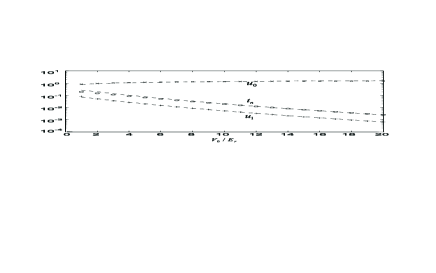
Figure 1: The normalized atom tunnelling rate $t_{n}\equiv t_{\mathbf{0}}^{\left(a\right)}/E_{r}$ (the subscript $\mathbf{0}$ means the lowest band), and the normalized overlaps between the atomic and the molecular Wannier functions $u_{0}\equiv\sqrt{\lambda/2}\int\left(w_{0}^{\left(m\right)}\left(x\right)\right)^{\ast}\left(w_{0}^{\left(a\right)}\left(x\right)\right)^{2}dx$ (on-site) and $u_{1}\equiv\sqrt{\lambda/2}\int\left(w_{0}^{\left(m\right)}\left(x\right)\right)^{\ast}w_{0}^{\left(a\right)}\left(x\right)w_{0}^{\left(a\right)}\left(x+\lambda/2\right)dx$ (neighboring sites) shown as a function of the lattice depth $V_{0}$ in the unit of the atom recoil energy $E_{r}$. The “o”,“$\times$”,“+” points denote the exact results from the numerical calculation, and the dashed curves show the fits from the formula $t_{n}\simeq\left(3.5/\sqrt{\pi}\right)\left(V_{0}/E_{r}\right)^{3/4}\exp\left(-2\sqrt{V_{0}/E_{r}}\right)$, $u_{0}\simeq 0.77\left(V_{0}/E_{r}\right)^{1/4}$, $u_{1}\simeq 0.52\left(V_{0}/E_{r}\right)^{3/4}\exp\left(-2\sqrt{V_{0}/E_{r}}\right)$.

The above Hamiltonian seems extremely complicated, however, we show now that under typical experimental conditions it can be dramatically simplified. To make this possible, first we note there are several different energy scales in this system, including the on-site interaction energy $E_{on}\sim c_{0;\mathbf{pss}^{\prime}}^{\left(am\right)}$, the band gap $E_{bg}\sim 2\sqrt{V_{0}E_{r}}$, the off-site interaction energy $E_{off}\sim c_{1;\mathbf{pss}^{\prime}}^{\left(am\right)}$, and the atom tunnelling rate $E_{t}\sim t_{\mathbf{p}}^{\left(a\right)}$. In experiments, the energy scale set by $E_{on},E_{bg}$ is typically much higher than the one set by $E_{off},E_{t}$. So we take the approximation $\left(E_{on},E_{bg}\right)\gg\left(E_{off},E_{t}\right)$. In this case, we can first solve the single-site Hamiltonian $H_{i}=\sum_{\mathbf{p}}\left[\left(\epsilon_{\mathbf{p}}^{\left(m\right)}+\nu_{b}\right)b_{i\mathbf{p}}^{\dagger}b_{i\mathbf{p}}+\sum_{\mathbf{\sigma}}\epsilon_{\mathbf{p}}^{\left(a\right)}a_{i\mathbf{p}\sigma}^{\dagger}a_{i\mathbf{p}\sigma}\right]+\sum_{\mathbf{pqs}}\left(c_{0;\mathbf{pss}^{\prime}}^{\left(am\right)}b_{i\mathbf{p}}^{\dagger}a_{i\mathbf{s}\uparrow}a_{i\mathbf{s}^{\prime}\downarrow}+h.c.\right)+\sum_{\mathbf{pqss}^{\prime}}c_{0;\mathbf{pqss}^{\prime}}^{\left(aa\right)}a_{i\mathbf{p}\downarrow}^{\dagger}a_{i\mathbf{q}\uparrow}^{\dagger}a_{i\mathbf{s}\uparrow}a_{i\mathbf{s}^{\prime}\downarrow}$ on the site $i$. We assume that the average atom filling number $\overline{n}$ of the lattice is smaller than $2$. If a site has a single atom on the $p$th band, its energy is just given by $\epsilon_{\mathbf{p}}^{\left(a\right)}$. If two atoms occupy the same site, they will form a local dressed molecule state, which in general can be written in the form $\left|\Psi_{i\mu}\right\rangle=d_{i\mu}^{\dagger}\left|0\right\rangle$, where $\left|0\right\rangle$ denotes the vacuum state and the dressed molecule creation operator $d_{i\mu}^{\dagger}\equiv\sum_{\mathbf{p}}\chi_{\mu\mathbf{p}}b_{i\mathbf{p}}^{\dagger}+\sum_{\mathbf{pq}}\gamma_{\mu\mathbf{pq}}a_{i\mathbf{p}\downarrow}^{\dagger}a_{i\mathbf{q}\uparrow}^{\dagger}$. In this expression for $d_{i\mu}^{\dagger}$, the superposition coefficients $\chi_{\mu\mathbf{p}},\gamma_{\mu\mathbf{pq}}$, with the normalization $\sum_{\mathbf{p}}\chi_{\mu\mathbf{p}}^{\ast}\chi_{\mu^{\prime}\mathbf{p}}+\sum_{\mathbf{pq}}\gamma_{\mu\mathbf{pq}}^{\ast}\gamma_{\mu^{\prime}\mathbf{pq}}=\delta_{\mu\mu^{\prime}}$, are determined by solving the Schrodinger equation $H_{i}\left|\Psi_{i\mu}\right\rangle=E_{\mu}\left|\Psi_{i\mu}\right\rangle$ note1 , where $\mu$ labels different eigenstates with the corresponding eigen-energy $E_{\mu}$. This kind of two-particle equation has been solved in Ref. 7 with a Harmonic approximation to the potential well. Here, we only need to mention two general features of the local dressed molecule states: first, the eigen-energies $E_{\mu}$ of the dressed molecule can be tuned by the external magnetic field $B$ through their dependence on $\nu_{b}$, although such a dependence is in general nonlinear; second, the energy difference between the adjacent eigenvalues $E_{\mu}$ is typically of the order of the band gap energy $E_{bg}$.

We consider the case with one of the eigen-energies, say $E_{\mu_{0}}$, pretty close to the two-atom free energy $2\epsilon_{\mathbf{p}_{0}}^{\left(a\right)}$ on a certain band $\mathbf{p}_{0}$, i.e., we tune the magnetic field $B$ to satisfy the condition $\left|E_{\mu_{0}}\left(B\right)-2\epsilon_{\mathbf{p}_{0}}^{\left(a\right)}\right|\ll E_{bg}$, as illustrated in Fig. 2. The $\mu_{0}$ and $\mathbf{p}_{0}$ can be chosen respectively as the ground state of the dressed molecule and the lattice lowest band, although they are not subject to such a restriction. Under the above condition, if the atoms start in the band $\mathbf{p}_{0}$, their state evolution will be restricted in the Hilbert subspace involving only the excitations of the modes $d_{i\mu_{0}}^{\dagger}$ and $a_{i\mathbf{p}_{0}\sigma}^{\dagger}$, as all the other states are significantly detuned by a energy scale of $\left(E_{on},E_{bg}\right)$ which is much larger than $\left(E_{off},E_{t}\right)$ note2 . So each site can only take four possible states, given by $\left|0\right\rangle$, $\left|\sigma\right\rangle\equiv a_{i\mathbf{p}_{0}\sigma}^{\dagger}\left|0\right\rangle$ $\left(\sigma=\uparrow,\downarrow\right)$, and $\left|d\right\rangle\equiv d_{i\mu_{0}}^{\dagger}\left|0\right\rangle$. We can then project the full Hamiltonian $H=H_{0}+H_{I}$ into the physical subspace specified by the projector $P\equiv\bigotimes_{i}P_{i}$, with $P_{i}\equiv\left|0\right\rangle_{i}\left\langle 0\right|+\left|\uparrow\right\rangle_{i}\left\langle\uparrow\right|+\left|\downarrow\right\rangle_{i}\left\langle\downarrow\right|+\left|d\right\rangle_{i}\left\langle d\right|$. After such a projection, the effective Hamiltonian $H_{eff}\equiv PHP$ takes the form

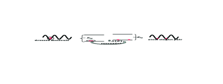
Figure 2: Illustration of resonance between the local dressed molecules and the atom valence bonds on neighboring sites.

$$H_{eff} = \sum_{i}\Delta\left(B\right)d_{i}^{\dagger}d_{i}+\sum_{i}\sum_{j\in N\left(i\right)}\left[\left(gd_{i}^{\dagger}\left(a_{i\uparrow}a_{j\downarrow}-a_{i\downarrow}a_{j\uparrow}\right)+h.c.\right)+t_{d}Pd_{i}^{\dagger}d_{j}P\right]$$ (2)

$$+\sum_{i}\sum_{j\in N\left(i\right)}\left[t_{a}\sum_{\sigma}Pa_{i\sigma}^{\dagger}a_{j\sigma}P+t_{da}\sum_{\sigma}d_{i}^{\dagger}d_{j}a_{j\sigma}^{\dagger}a_{i\sigma}+c_{d}n_{id}n_{jd}+c_{a}\left(n_{i}n_{j}/4-\mathbf{s}_{i}\cdot\mathbf{s}_{j}\right)\right],$$

where we have used the simplified notations $d_{i}\equiv d_{i\mu_{0}}$, $a_{i\sigma}=a_{i\mathbf{p}_{0}\sigma}$, $\Delta\left(B\right)\equiv E_{\mu_{0}}\left(B\right)-2\epsilon_{\mathbf{p}_{0}}^{\left(a\right)}$ (the atom energy zero point  has been shifted to coincide with $\epsilon_{\mathbf{p}_{0}}^{\left(a\right)}$), and defined the number and the spin operators $n_{id}\equiv d_{i}^{\dagger}d_{i}$, $n_{i}\equiv\sum_{\sigma}a_{i\sigma}^{\dagger}a_{i\sigma}$, $\mathbf{s}_{i}\equiv\sum_{\sigma\sigma^{\prime}}a_{i\sigma}^{\dagger}\mathbf{\sigma}_{\sigma\sigma^{\prime}}a_{i\sigma^{\prime}}/2$ with the Pauli matrix $\mathbf{\sigma=}\left(\sigma_{x},\sigma_{y},\sigma_{z}\right)$. The parameters in the Hamiltonian $H_{eff}$ are given by $g=\gamma_{\mu_{0}\mathbf{p}_{0}\mathbf{p}_{0}}^{\ast}t_{\mathbf{p}_{0}}^{\left(a\right)}/2$ $+\sum_{\mathbf{q}}\chi_{\mu_{0}\mathbf{q}}^{\ast}c_{1;\mathbf{qp}_{0}\mathbf{p}_{0}}^{\left(am\right)}+\sum_{\mathbf{qs}}\gamma_{\mu_{0}\mathbf{qs}}^{\ast}c_{1;\mathbf{qsp}_{0}\mathbf{p}_{0}}^{\left(aa\right)}$, $t_{d}=\sum_{\mathbf{q}}\left|\chi_{\mu_{0}\mathbf{q}}\right|^{2}t_{\mathbf{q}}^{\left(m\right)}$ $+2\mathop{\rm Re}\nolimits(\sum_{\mathbf{qss}^{\prime}}\chi_{\mu_{0}\mathbf{q}}^{\ast}c_{2;\mathbf{qss}^{\prime}}^{\left(am\right)}\gamma_{\mu_{0}\mathbf{s}^{\prime}\mathbf{s}})+\sum_{\mathbf{pqss}^{\prime}}\gamma_{\mu_{0}\mathbf{pq}}^{\ast}c_{2;\mathbf{pqss}^{\prime}}^{\left(aa\right)}\gamma_{\mu_{0}\mathbf{s}^{\prime}\mathbf{s}}$, $t_{a}=t_{\mathbf{p}_{0}}^{\left(a\right)}$, $t_{da}=-\sum_{\mathbf{q}}\left|\gamma_{\mu_{0}\mathbf{qp}_{0}}\right|^{2}t_{\mathbf{q}}^{\left(a\right)}$ $-2\mathop{\rm Re}\nolimits(\sum_{\mathbf{qs}}\chi_{\mu_{0}\mathbf{q}}^{\ast}c_{1;\mathbf{qp}_{0}\mathbf{s}}^{\left(am\right)}\gamma_{\mu_{0}\mathbf{sp}_{0}})-2\mathop{\rm Re}\nolimits(\sum_{\mathbf{pqs}}\gamma_{\mu_{0}\mathbf{pq}}^{\ast}c_{1;\mathbf{pqp}_{0}\mathbf{s}}^{\left(aa\right)}\gamma_{\mu_{0}\mathbf{sp}_{0}})$, $c_{d}=\sum_{\mathbf{pp}^{\prime}\mathbf{qq}^{\prime}\mathbf{ss}^{\prime}}\gamma_{\mu_{0}\mathbf{pp}^{\prime}}^{\ast}\gamma_{\mu_{0}\mathbf{q}^{\prime}\mathbf{q}}^{\ast}c_{3;\mathbf{pqss}^{\prime}}^{\left(aa\right)}\gamma_{\mu_{0}\mathbf{sp}^{\prime}}\gamma_{\mu_{0}\mathbf{q}^{\prime}\mathbf{s}^{\prime}}$, $c_{a}=c_{3;\mathbf{p}_{0}\mathbf{p}_{0}\mathbf{p}_{0}\mathbf{p}_{0}}^{\left(aa\right)}$.

The Hamiltonian $H_{eff}$ represents an effective single-band model, but it has incorporated multi-band information into its parameters through the structure coefficients $\chi_{\mu_{0}\mathbf{p}}$,$\gamma_{\mu_{0}\mathbf{pq}}$ of the local dressed molecules. This Hamiltonian contains no on-site interactions as they have been exactly taken into account into the structure of the dressed molecules. As one tunes $\Delta\left(B\right)$ through the magnetic field, the Hamiltonian $H_{eff}$ describes a crossing resonance between the local dressed molecules $d_{i}$ and the atomic valence bonds $a_{i\uparrow}a_{j\downarrow}-a_{i\downarrow}a_{j\uparrow}$ on the neighboring sites. This resonance may have a richer structure than the conventional Feshbach resonance between the bare molecules and the free atoms as first, the dressed molecule here has been a complicated superposition of the bare molecules and the local Cooper pairs, and second, the resonance to valence bonds on neighboring sites may introduce rich configurations depending on the lattice geometry.

The Hamiltonian $H_{eff}$ supports rich physics. Its detailed study will be presented elsewhere. Here, we investigate $H_{eff}$ in two limiting cases with the detuning $\left|\Delta\left(B\right)\right|$ significantly larger than the neighboring coupling rate $g$. We can see already rich phase diagrams from $H_{eff}$ in these limiting cases. First, we consider the case with the population dominantly in the atoms and the local dressed molecules only virtually excited due to the large detuning $\Delta\left(B\right)$ (the lattice filling number $\overline{n}\leq 1$ in this case). We can then reduce $H_{eff}$ to an effective Hamiltonian involving only the atomic operators $a_{i\sigma}$. For this purpose, we define the projection operator $P_{a}\equiv\bigotimes_{i}P_{i}^{\left(a\right)}$ with $P_{i}^{\left(a\right)}\equiv\left|0\right\rangle_{i}\left\langle 0\right|+\left|\uparrow\right\rangle_{i}\left\langle\uparrow\right|+\left|\downarrow\right\rangle_{i}\left\langle\downarrow\right|$, and keep the terms up to the order of $\left|g\right|^{2}/\Delta\left(B\right)$ in the projection. The reduced Hamiltonian can be derived through either the second-order perturbation or a canonical transformation 11 , and it takes the form of the famous $t$-$J$ model

$$H_{tJ}=\sum_{i;j\in N\left(i\right)}\left[t_{a}\sum_{\sigma}P_{a}a_{i\sigma}^{\dagger}a_{j\sigma}P_{a}+J\left(\mathbf{s}_{i}\cdot\mathbf{s}_{j}-n_{i}n_{j}/4\right)\right],$$ (3)

where the parameter $J=-c_{a}-2\left|g\right|^{2}/\Delta\left(B\right)$ note3 . In $H_{tJ}$, we have not included the $3$-site nonlinear tunnelling $H_{3}=\left[-\left|g\right|^{2}/\Delta\left(B\right)\right]\sum_{i}\sum_{j,k\in N\left(i\right)}\left(a_{i\uparrow}^{\dagger}a_{k\downarrow}^{\dagger}-a_{i\downarrow}^{\dagger}a_{k\uparrow}^{\dagger}\right)\times\left(a_{i\uparrow}a_{j\downarrow}-a_{i\downarrow}a_{j\uparrow}\right)$, which is usually omitted in the literature note4 . The $t$-$J$ model plays a fundamental role in study of high $T_{c}$ superconductivity 10 ; 11 ; 12 . Depending on the ratio $t_{a}/J$, the atom filling $\overline{n}$, and the lattice dimension and geometry, the $t$-$J$ model shows rich phase diagrams, including, for instance, the atomic anti-ferromagnetic phase, the $d$-wave superconductivity 14 , and likely the resonating valence bond (RVB) states 10 ; 11 . The $t$-$J$ model was previously derived as the strong interaction limit of the Hubbard model 10 ; 12 . Here, although our basic Hamiltonian $H_{eff}$ does not resemble any forms of the Hubbard model, we get exactly the same reduced Hamiltonian as the $t$-$J$ model; furthermore, our atomic realization of the $t$-$J$ model is not subject to the constraint $J\ll t_{a}$ as is the case from the Hubbard model. All the parameters here can be experimentally tuned in the full range, which, together with the easy control of the lattice dimension and geometry, makes this system the ideal test bed for many outstanding predictions and hypotheses associated with the $t$-$J$ model.

We now consider another limiting case of our basic Hamiltonian $H_{eff}$ with the population dominantly in the dressed molecules and the atoms only virtually excited (still, $\left|\Delta\left(B\right)\right|\gg\left|g\right|$). In this case, we define the molecule projection operator $P_{m}\equiv\bigotimes_{i}P_{i}^{\left(m\right)}$ with $P_{i}^{\left(m\right)}\equiv\left|0\right\rangle_{i}\left\langle 0\right|+\left|d\right\rangle_{i}\left\langle d\right|$. Up to the order of $\left|g\right|^{2}/\Delta\left(B\right)$, the reduced Hamiltonian for the dressed molecules has the form

$$H_{m}=\sum_{i}\left[\Delta^{\prime}n_{id}+\sum_{j\in N\left(i\right)}\left(t_{d}^{\prime}P_{m}d_{i}^{\dagger}d_{j}P_{m}+c_{d}^{\prime}n_{id}n_{jd}\right)\right]$$ (4)

where $t_{d}^{\prime}=t_{d}+2\left|g\right|^{2}/\Delta\left(B\right),$ $c_{d}^{\prime}=c_{d}-2\left|g\right|^{2}/\Delta\left(B\right)$, and $\Delta^{\prime}=\Delta\left(B\right)+2n_{c}\left|g\right|^{2}/\Delta\left(B\right)$ ($n_{c}$ is the lattice coordination number). This Hamiltonian describes hard-core bosons with neighboring interactions, and it is identical to the magnetic XXZ model $H_{XXZ}=\left(t_{d}^{\prime}/4\right)\sum_{i}\left[B_{eff}Z_{i}+\sum_{j\in N\left(i\right)}\left(X_{i}X_{j}+Y_{i}Y_{j}+\delta_{z}Z_{i}Z_{j}\right)\right],$ $\left(\delta_{z}=c_{d}^{\prime}/t_{d}^{\prime}\text{, }B_{eff}=2\left(\Delta^{\prime}+n_{c}c_{d}^{\prime}\right)/t_{d}^{\prime}\right)$ for the effective Pauli operators $X_{i},Y_{i},Z_{i}$ through the following mapping: $X_{i}\equiv P_{m}\left(d_{i}+d_{i}^{\dagger}\right)P_{m}$, $Y_{i}\equiv iP_{m}\left(d_{i}-d_{i}^{\dagger}\right)P_{m}$, $Z_{i}\equiv 2d_{i}^{\dagger}d_{i}-1$ 14 ; 6 . The phase diagram of the XXZ model is know pretty well. For instance, it has the ferromagnetic, the canted XY, and the anti-ferromagnetic phases 15 , which correspond respectively to the Mott state, the superfluidity state, and the checkerboard state (one occupation every other sites) of the dressed molecules. It also has more exotic quantum phases (RVB spin liquids etc.) if the lattice geometry induces frustration of the above spin orders 16 .

In summary, we have derived the effective Hamiltonian for fermionic atoms in an optical lattice across broad Feshbach resonance, taking into account of both the multi-band configurations and the direct neighboring interactions. In certain limits, this Hamiltonian is reduced to either the $t$-$J$ model for the fermionic atoms or the XXZ model for the local dressed molecules. The latter two models connect to many fundamental physics associated with many-body systems.

This work was supported by the NSF awards (0431476), the ARDA under ARO contracts, and the A. P. Sloan Fellowship.

References

• (1) C.A. Regal, M. Greiner and D.S. Jin, Phys. Rev. Lett. 92, 040403 (2004); M.W. Zwierlein et al., Phys. Rev. Lett. 92, 120403 (2004); C. Chin et al., Science 305, 1128 (2004); J. Kinast et al., Science 307, 1296 (2005); M.W. Zwierlein et al., Nature 435, 1047 (2005); M. Holland et al., Phys. Rev. Lett. 87, 120406 (2001); Y. Ohashi and A. Griffin, Phys. Rev. Lett. 89, 130402 (2002).
• (2) M. Greiner, et al., Nature 415, 39 (2002); C. Orzel, et al., Science 291, 2386 (2001); D. Jaksch, et al., Phys. Rev. Lett. 81, 3108 (1998).
• (3) For a review, see R.A. Duine and H.T.C. Stoof, Phys. Rep. 396, 115 (2004); Q. Chen et al., Phys. Reports 412, 1 (2005).
• (4) For a review, see D. Jaksch, P. Zoller, cond-mat/0410614.
• (5) D. B. M. Dickerscheid et al., Phys. Rev. A 71, 043604 (2005); Phys. Rev. Lett. 94, 230404 (2005).
• (6) L. Carr and M. Holland, cond-mat/0501156; F. Zhou, cond-mat/0505740.
• (7) R. B. Diener, T.-L. Ho, cond-mat/0507253; cond-mat/0507255.
• (8) M. Kohl et al., Phys. Rev. Lett. 94, 080403 (2005).
• (9) K. Xu et al., cond-mat/0507288.
• (10) P. W. Anderson, Science 235, 1196 (1987).
• (11) A. Auerbach, Interacting Electrons and Quantum Magnetism, Springer-Verlag, New York (1994).
• (12) F. C. Zhang, T. M. Rice, Phys. Rev. B 37, 3759 (1988).
• (13) L.-M. Duan, Euro. Phys. Lett. 67, 721 (2004).
• (14) In solving this two-atom Schrodinger equation, one needs to apply some renormalization procedure as has been specified in Ref. 7 .
• (15) These other states include $3$ or more atom occupations of a single site, which take an energy cost typically of the order of $E_{on}$, and thus will not be excited in our considered case.
• (16) In this expression of $J$, we have included the virtual excitation contribution from only the nearest dressed molecule level. If the detuning $\Delta\left(B\right)$ becomes comparable with the band gap $E_{bg}$, one should include in $J$ the virtual excitation contributions from several nearby dressed molecule levels, but the reduced Hamiltonian for the atoms still takes the form of the $t$-$J$ model.
• (17) This omission is based on the believe that the main physics of the $t$-$J$ model is caught by the competition between the $t$ and $J$ terms, and the $3$-site tunneling is not as important as the $t$ term, see, e.g., the discussion on page 27 in Ref. 11 .
• (18) R. Micnas, J. Ranninger, and S. Robaszkiewicz, Rev. Mod. Phys. 62, 113 (1990).
• (19) L.-M. Duan, E. Demler, M. D. Lukin, Phys. Rev. Lett. 91, 090402 (2003).
• (20) For a review, see C. Lhuillier, G. Misguich, cond-mat/0109146.