Numerical simulation of the stochastic dynamics of inclusions in biomembranes in presence of surface tension

Abstract

The stochastic dynamics of inclusions in a randomly fluctuating biomembrane is simulated. These inclusions can represent the embedded proteins and the external particles arriving at a cell membrane. The energetics of the biomembrane is modelled via the Canham-Helfrich Hamiltonian. The contributions of both the bending elastic-curvature energy and the surface tension of the biomembrane are taken into account. The biomembrane is treated as a two-dimensional sheet whose height variations from a reference frame is treated as a stochastic Wiener process. The lateral diffusion parameter associated with this Wiener process coupled with the longitudinal diffusion parameter obtained from the standard Einsteinian diffusion theory completely determine the stochastic motion of the inclusions. It is shown that the presence of surface tension significantly affects the overall dynamics of the inclusions, particularly the rate of capture of the external inclusions, such as drug particles, at the site of the embedded inclusions, such as the embedded proteins.
PACS: 87.20; 34.20; 87.22BT
Keywords: Biomembrane computational modelling, Stochastic simulation, Canham-Helfrich Hamiltonian, Surface tension, Inclusion diffusion.

1 Introduction

Amphiphilic molecules, such as lipids and proteins, are composed of hydrophilic heads and hydrophobic hydrocarbon-based chains. They can self-assemble themselves into a variety of exotic structures when placed in an aqueous environment [1]. One such structure is the biological membrane composed of a bilayer of phospholipid molecules. Biomembranes have very interesting spatial dimensions. Their thicknesses can vary up to few nano-meters, but their linear sizes can take up to tens of micro-meters. They can, therefore, be regarded as highly flexible fluid-like two-dimensional (2D) sheets embedded in three-dimensional embedding space.

Biomembranes form large encapsulating bags, called vesicles, because open sheet-like configurations would involve a large energy along the hydrophobic edges [2]. They play a very significant role in many of the life’s processes, since not only they act as barriers to maintain the structural integrity of cells, but also provide the functional environment for many of the embedded proteins that penetrate the biomembrane thicknesses and act as ion transport channels to the interior of the cells [3].

Biomembranes can be studied from three perspectives [2], namely (i) their molecular architecture, focusing on their material properties, (ii) as statistical-mechanical systems displaying a very rich and exotic variety of configurations as 2D surfaces, and (iii) their functioning in biological systems.

In our previous work [4], as well as in this paper, we have been interested in biomembranes from the second perspective (ii), and in particular we have been concerned with computational modelling of the diffusion dynamics of objects (inclusions) existing within and on the surface of stochastically fluctuating biomembranes. The stochastic fluctuations of the biomembranes can originate from thermal fluctuations. They promote shape fluctuations and shape transformations in biomembranes. One such shape transformation, observed under video microscopy, is the so-called budding transition in which a change of temperature from $T=27.2$ C to $T=41$ C resulted in a change of shape of a spherical vesicle into a prolate ellipsoid, and the eventual fission of the biomembrane [2].

Two types of inclusion can be considered in a biomembrane. These are the internal inclusions, or the biomembrane’s own inclusions, which we refer to as the M-type, and the external inclusions, which we refer to as the S-type. The S-type inclusions, such as drug particles, arrive at the biomembrane from outside. The M-type inclusions are the embedded objects, such as proteins, or ion channels, that are an integral part of a biomembrane. Although embedded in the amphiphilic environment, these inclusions are mobile and can freely diffuse across the biomembrane.

The M-type inclusions penetrate the thickness of the biomembrane, and hence disturb its geometry locally by forcing the amphiphilic bilayer to adjust its thickness locally so as to match its hydrophobic regions with those of the inclusions [5, 6], as shown in Fig.1. This change in the local geometry generates perturbations in the fluid-like biomembrane structure and these perturbations, in turn, lead to both short- and long-range biomembrane-induced forces between the inclusions. Such geometro-dynammic forces affect the behaviour of inclusions in a biomembrane in addition to any other forces, such as direct molecular forces, that may operate between these inclusions, or between them and the embedding biomembrane. If these induced perturbations are of long wavelength, then they generate long-range forces, otherwise, they lead to short-range forces that act in the immediate vicinity of the inclusions.

The deformation in local geometry is one of the three deformation modes of a biomembrane. Since a biomembrane is surrounded by solutions, such as water, the surface tension existing at the biomembrane-water interface changes the overall surface area of the biomembrane. This change constitutes the second mode of deformation. The third mode is associated with the bending property of a biomembrane, which is associated with its elastic-curvature property. It is this property that distinguishes a fluid-like biomembrane sheet from a simple fluid sheet in which surface tension alone dominates the surface dynamics. [2, 7].

In the studies concerned with the inclusion-induced local deformations, two approaches have been adopted to model these deformations. In one model [8, 9, 10, 11, 12] the biomembrane energy is taken to be the sum of the energy due to molecular compression/expansion brought about by the change in local geometry and the energy due to the change in the overall surface area, while in another model [5, 13] the contribution of the bending energy is also included. The first model shows that the inclusion- induced deformations force a change of thickness in local geometry which decays exponentially from the inclusion-imposed value to the equilibrium thickness of the biomembrane. This is shown schematically in Fig.1 for two rod-like inclusions. The second model shows that the contribution of bending energy could significantly affect the deformation profile at the inclusion boundary, as well as the biomembrane-induced interactions.

The S-type inclusions arrive from the outside of the biomembrane and reside on its surface. Fig.2 represents a schematic representation of two such inclusions lying on the surface of a biomembrane sheet.

In our previous work [4], we performed a computational simulation of the diffusion dynamics of both the external and internal inclusions in a stochastically fluctuating biomembrane in which the biomembrane energy was solely described in terms of the bending elastic-curvature energy. Furthermore, in that work we considered only the contribution of the lateral component of the diffusion coefficient of the inclusions, brought about by the lateral fluctuations in the height of the biomembrane, to the motion of the inclusions. In the present paper, we have extended our previous modelling on two levels. Firstly, have also included the contribution of biomembrane’s surface tension to the stochastic dynamics of inclusions, and secondly, the contribution of the longitudinal component of the diffusion coefficient has also been included. The combination of these two components now forms the diffusion coefficient governing the motion of the inclusions. Various forms of this combination has been tested. It is seen that the dynamics of inclusions is significantly affected by the presence of surface tension.

2 Energetics of the biomembrane in presence of surface tension

Biomembranes are characterized by their bending rigidity [14, 15, 16] and they strongly undulate under thermal fluctuations. Consequently, in studying biomembranes, surface tension effects are usually neglected and only the bending rigidity is considered as the source controlling their shape and fluctuations. However, surface tension can contribute significantly to the energy of a biomembrane if geometrical constraints [17] or external perturbations, due to the attached proteins in biological systems, are introduced [18]. For instance, it has been shown that [19] the area dependence of surface tension can lead to a stable hole of finite size in the biomembrane. Furthermore, interesting phenomena have been observed when biomembranes are perturbed by the action of microscopes [20], or in recent years by laser tweezers [21]. The typical effect of such tweezers on an initially flaccid biomembrane has been reported [21] where the application of the laser tweezers on a vesicle over few minutes caused the shape fluctuations of the biomembrane to disappear. With this disappearance, the biomembrane became quite taut, indicating the presence of a non-negligible surface tension, $\sigma\geq 10^{-3}$erg/cm². This tension caused the expulsion of a vesicle from inside of another vesicle. Such an spontaneous expulsion is quite surprising [19], since it involves the opening of a large hole, of energy much larger than the thermal energy. In comparison, using mechanical manipulation, rather than tweezers, of very large vesicles, tensions as low as, $\sigma\geq 10^{-6}$erg/cm² [20] have also been recorded. It is, therefore, quite reasonable to assume that surface tension in the above range plays a significant role in the dynamic behaviour of a biomembrane. These experiments, therefore, show that a realistic study of the energetics of biomembranes should include not only the bending rigidity, but also the effect of the surface tension.

The free elastic energy of a symmetric, nearly flat, biomembrane sheet is described by the Canham-Helfrich Hamiltonian [22, 23]

$${\cal H}=\int d^{2}\sigma\sqrt{g}\left\{\sigma_{0}+2\kappa H^{2}+\bar{\kappa}K\right\},$$ (1)

where

$$K = \mbox{det}(K_{ij})=\frac{1}{R_{1}R_{2}},$$

$$H = \frac{1}{2}\mbox{Tr}(K_{ij})=\frac{1}{2}\left(\frac{1}{R_{1}}+\frac{1}{R_{2}}\right),$$

are the Gaussian and mean curvatures of the sheet respectively, $R_{1}$ and $R_{2}$ are the principal radii of the sheet, $\sigma_{0}$ is the surface tension, $\kappa$ is the bending rigidity, $\bar{\kappa}$ is the Gaussian rigidity, $g$ is the determinant of the metric tensor and $\sigma=(\sigma_{1},\sigma_{2})$ is the local coordinate defined on the sheet. The last term on the RHS of (1) is, by Gauss-Bonnet theorem, a topological invariant and does not affect the dynamics of the biomembrane if there were no changes in its topology. We will, therefore, ignore this term as we assume that no such changes occur. We thus have

$${\cal H}=\int d^{2}\sigma\sqrt{g}\left\{\sigma_{0}+2\kappa H^{2}\right\}.$$ (2)

To facilitate the study of a nearly flat biomembrane, whose free energy is given by (2), it is convenient to consider it to be parallel to the $(x_{1}-x_{2})$ plane, regarded as the reference plane. The position of a point on the biomembrane can then be described by a single-valued height function, $h$, representing the position of a point on a fluctuating, nearly flat, sheet relative to the reference plane. In this, the so-called Monge representation [2], equation (2) is written as

$${\cal H}=\frac{1}{2}\int d^{2}x\left\{\kappa(\nabla^{2}h)^{2}+\sigma_{0}(\nabla h)^{2}\right\}.$$ (3)

In this form, the Hamiltonian is expressed solely in terms of the height function, $h$, and its derivatives. We remark that in our previous work [4] the contribution of the second term on the RHS of (3) was not included as we did not consider the contribution of the surface tension $\sigma_{0}$. The Hamiltonian in (3) describes the energetics of the biomembrane from which we obtain the stochastic lateral motion of both the M-type and the S-type inclusions.

2.1 Computation of the lateral diffusion coefficient of inclusions

Let us first consider the lateral stochastic motion of the inclusions, i.e. that component of the motion which is associated with the changes in $h(x_{1},x_{2})$. One way to introduce stochastic behaviour into the dynamics of the biomembrane is to treat $h$, obtained from (3), as a stochastically fluctuating Wiener process. Evidently, this stochastic behaviour is communicated to the inclusions residing inside, as well as on the surface, of the biomembrane.

To derive the lateral diffusion coefficient, $D_{\bot}$, associated with the random changes in the height function, we first need to obtain the the height-height correlation function of the biomembrane in real space. This is obtained from (3) by first going over to the Fourier representation of $h$, i.e.

$$h({\bf x})=\int\frac{d^{2}q}{(2\pi)^{2}}h(\bf q)e^{i{\bf q}\cdot{\bf x}}\,,$$ (4)

where ${\bf x}=(x_{1},x_{2})$ is the vector position of the point on the biomembrane. Consequently, (3) now reads

$${\cal H}=\frac{1}{2}\int\frac{d^{2}q}{(2\pi)^{2}}\left\{\kappa q^{4}+\sigma_{0}q^{2}\right\}h({\bf q})h^{\ast}({\bf q})\,,$$ (5)

where $*$ denotes the complex conjugate. The static height-height correlation function can be calculated, with the result

$$\langle h({\bf q};0)h^{\ast}({\bf q^{\prime}};0)\rangle=\left(\frac{k_{\tiny\mbox{B}}T}{\kappa q^{4}+\sigma_{0}q^{2}}\right)(2\pi)^{2}\delta({\bf q}-{\bf q}^{\prime}),$$ (6)

where the averaging is done with respect to the Boltzmann weight factor $\mbox{exp}(-{\cal H}/k_{\tiny\mbox{B}}T)$, with $k_{\tiny\mbox{B}}$ being the Boltzmann constant. The corresponding dynamic correlation function can be written as

$$h({\bf q};t)=h({\bf q};0)e^{-\gamma(q)t},$$

leading to

$$\langle h({\bf q};t)h^{\ast}({\bf q^{\prime}};0)\rangle=e^{-\gamma(q)t}\left(\frac{k_{B}T}{\kappa q^{4}+\sigma_{0}q^{2}}\right)(2\pi)^{2}\delta({\bf q}-{\bf q}^{\prime}),$$ (7)

where the damping factor, $\gamma(q)$, reflecting the long-range character of the hydrodynamic damping, is given by [2]

$$\gamma(q)=\frac{1}{4\eta}\left(\kappa q^{3}+\sigma_{0}q\right).$$ (8)

Here, $\eta$ denotes the coefficient of viscosity of the fluid surrounding the biomembrane. We note that in the absence of $\sigma_{0}$, (8) reduces to the damping factor given in equation (13) of our previous work [4]. In real space, the Fourier transform of (7) is given by

$$\langle h({\bf x};t)h({\bf x};0)\rangle=\int\int\frac{d^{2}q}{(2\pi)^{2}}\frac{d^{2}q^{\prime}}{(2\pi)^{2}}\langle h({\bf q};t)h^{*}({\bf q^{\prime}};0)\rangle e^{-{\bf x}.({\bf q}-{\bf q^{\prime})}}\,,$$ (9)

or substituting from (7) and (8)

$$\langle h({\bf x};t)h({\bf x};0)\rangle=\frac{1}{2\pi\beta}\int_{\frac{1}{L}}^{\frac{1}{a}}dq\frac{e^{-\frac{1}{4\eta}(\kappa q^{3}+\sigma_{0}q)t}}{\kappa q^{3}+\sigma_{0}q}\,,$$ (10)

where $L$ is the linear size of the biomembrane and $a$ is a molecular cut-off, of the order of nanometers, and $\beta=\frac{1}{k_{\tiny\mbox{B}}T}$. The Fourier transform expression in (10) is quite complicated to perform and it was computed in the Mathematica software [24] by expanding the integrand and computing it term by term. The final analytical result, consisting of many terms, need not be quoted here and can be obtained from the authors upon request. In our previous work [4], the Fourier transform to real space was performed under simplifying assumptions regarding the transform of the damping factor term $\gamma$. In this paper, however, no assumptions were applied and the transform was fully computed.

Now, treating $h$ as a stochastic Wiener process implies that the mean and variance are given by

$$\langle h(x_{1},x_{2};t)\rangle = 0,$$ (11)

$$\langle h(x_{1},x_{2};t)h(x_{1},x_{2};0)\rangle = =2D_{\bot}t,$$ (12)

in which $D_{\bot}$, the diffusion constant associated with the random fluctuations in the height function at the local position $(x_{1},x_{2})$, represents a measure of these fluctuations. Such random fluctuations can cause a roughening of the biomembrane surface as has been observed in NMR experiments [25].

Consequently, since the biomembrane’s stochastic behaviour is transmitted to the inclusions, we can make the assumption that the centre of mass of an inclusion coinciding with the point $(x_{1},x_{2})$ on the biomembrane would also experience the same lateral fluctuations, whose measure is the same diffusion coefficient, $D_{\bot}$.

Therefore, the expression for $D_{\bot}$ for the inclusions in presence of surface tension can be obtained by comparing (10) and (12), leading to

$$D_{\bot}=\frac{1}{2t}\left[\frac{1}{2\pi\beta}\int_{\frac{1}{L}}^{\frac{1}{a}}dq\frac{e^{-\frac{1}{4\eta}(\kappa q^{3}+\sigma_{0}q)t}}{\kappa q^{3}+\sigma_{0}q}\right].$$ (13)

2.2 Computation of the longitudinal diffusion coefficient of inclusions

In addition to the lateral component of the diffusion coefficient, computed above, we also require the longitudinal component, $D_{\|}$, for both the S-type and the M-type inclusions. This coefficient is calculated via Einstein’s general model of Brownian dynamics [26] according to which

$$D_{\|}=\frac{1}{2Nst}\langle\sum_{i=1}^{N}\mid r_{i}(t)-r_{i}(0)\mid^{2}\rangle\,,$$ (14)

where $t$ is the delay (correlation) time, $\langle\cdots\rangle$ refers to averaging over time, $s$ is the dimensionality of diffusion space (2 in the present case) and $N$ is the number of inclusions. In the actual computation of $D_{\|}$, the time average is replaced with a summation over time origins from which the delay time is measured, so that (14) is written as [26]

$$D_{\|}=\frac{1}{2XNst}\sum_{k=1}^{X}\sum_{i=1}^{N}\left[\mid r_{i}(t_{k}+t)-r_{i}(t_{k})\mid^{2}\right]\,,$$ (15)

where $X$ is total number of available time origins.

2.3 Computation of the stochastic trajectories

In our present numerical simulations, just as in the previous study [4], the equations of motion of both the M-type and the S-type inclusions are described via the Ito stochastic calculus [28] whose stochastic differential equation is given by

$$d{\bf r}(t)={\bf A}[{\bf r}(t),t]+D_{t}^{1/2}d{\bf W}(t).$$ (16)

This equation describes the random trajectories, ${\bf r}(t)$, of the centres of mass of the inclusions in terms of a dynamical variable of the inclusions, ${\bf A}[{\bf r}(t),t]$, which is referred to as the drift velocity, and a term, $d{\bf W}(t)$, which is modelled by a Wiener process with the mean and variance given by

$$\langle d{\bf W}(t)\rangle = 0,\hskip 8.53581pt$$

$$\langle d{\bf W}_{i}(t)d{\bf W}_{j}(t)\rangle = 2\delta_{ij}dt.$$ (17)

In (16), $D_{t}$ represents the total diffusion coefficient of the inclusions. In this paper, following the prescription given by [27] for the Brownian motion of rod-like objects, we represent this coefficient by a linear combination of the lateral and longitudinal coefficients and, to test the various possibilities, consider the following different combinations

$$D_{t} = \frac{1}{2}D_{\bot}+\frac{1}{2}D_{\|}$$ (18)

$$= \frac{2}{3}D_{\bot}+\frac{1}{3}D_{\|}$$

$$= \frac{1}{3}D_{\bot}+\frac{2}{3}D_{\|}.$$

In the vicinity of an M-type inclusion, care should be exercised in using $D_{t}$. Near an M-type inclusion, localized exponentially-decaying deformation would occur in the membrane geometry [4, 5], as depicted in Fig.1. This implies that near such an inclusion we can scale the diffusion coefficient by an exponentially decaying function, i.e. if $r_{0}$ is the radius of an M-type inclusion, then within a circular region $R+r_{0}$, the modified diffusion coefficient could be modelled as

$$D_{mt}=D_{t}e^{\frac{-r_{0}}{R}}\,,$$ (19)

implying that when an S-type inclusion enters a region centered around an M-type inclusion, within the radius $R+r_{0}$, the diffusion coefficient goes over to $D_{mt}$ and, to a first approximation, this is how an M-type inclusion interacts with an S-type one.

The Ito equation (16) predicts the increment in position for a meso-scale time interval, $dt$, as a combination of deterministic and stochastic diffusive parts represented by the terms ${\bf A}[{\bf r}(t)]$ and $D_{t}^{1/2}d{\bf W}(t)$ respectively. This equation resembles the ‘position’ Langevin equation describing the Brownian motion of a particle [29]. The position Langevin equation corresponds to the long-time (diffusive time) configurational dynamics of a stochastic particle in which its momentum coordinates are in thermal equilibrium and hence can be removed from the equations of motion. Since we are interested in diffusive time scales as well, we can re-write (16) as

$$d{\bf r}(t)=\frac{D_{t}}{k_{B}T}{\bf F}(t)+D_{t}^{1/2}d{\bf W}(t),$$ (20)

where ${\bf F}(t)$ is the instantaneous systematic (Newtonian) force experienced by the centre of mass of the $i$th inclusion. This force can obtained from the inter-inclusion potentials, $V(R_{ij})$, according to

$${\bf F}_{i}=-\sum_{j>i}\nabla_{{\bf R}_{i}}V(R_{ij}).$$ (21)

Pertinent potentials have been constructed employing a statistical mechanics based on the Canham-Helfrich Hamiltonian. For the M-M interaction, this potential is given by [30, 31]

$$V^{T}_{\tiny\mbox{MM}}(R_{ij})=-k_{B}T\frac{12A^{2}}{\pi^{2}R_{ij}^{4}},$$ (22)

describing the biomembrane-mediated temperature-dependent long-range interactions between a pair of disk shape M-type inclusions that can freely tilt with respect to each other. For the S-S interaction, the potential is given by [32]

$$V^{T}_{\tiny\mbox{SS}}(R_{ij},\theta_{i},\theta_{j})=-k_{B}T\frac{L_{i}^{2}L_{j}^{2}}{128R^{4}_{ij}}\cos^{2}[2(\theta_{i}+\theta_{j})],$$ (23)

where $A=\pi r_{0}^{2}$ is the area of an M-type inclusion of radius $r_{0}$, $R_{ij}$ is the distance between the centres of mass of two inclusions $i$ and $j$, $L_{i}$ and $L_{j}$ are the lengths of two S-type inclusions making angles $\theta_{i}$ and $\theta_{j}$ respectively with the line joining their centres of mass (Fig.2) and $T$ is the biomembrane temperature. These expressions are derived for the rod-like inclusions that are assumed to be much more rigid than the ambient biomembrane so that these inclusions cannot move coherently with the biomembrane.

We performed numerical simulations of the space-time motion of inclusions described by (20) by adopting the following iterative scheme [33]

$$X(t+dt)=X(t)+\frac{D_{t}}{k_{B}T}F_{X}(t)dt+\sqrt{2D_{t}dt}\,R^{G}_{X},$$

(24)

$$Y(t+dt)=Y(t)+\frac{D_{t}}{k_{B}T}F_{Y}(t)dt+\sqrt{2D_{t}dt}\,R^{G}_{Y},$$

where $R^{G}_{X}$ and $R^{G}_{Y}$ are standard random Gaussian variables chosen separately and independently for each inclusion according to the procedure given in [29], and $F_{X}$, $F_{Y}$ are the $X$ and $Y$ components of the force $\bf F$. For the S-type inclusions, we treated the angles in (23) as independent stochastic variables described by

$$\theta(d+dt)=\theta(t)+\frac{D_{t}}{k_{B}TL^{2}}\tau(t)dt+\frac{1}{L}\sqrt{2D_{t}dt}\,\theta^{G},$$ (25)

where $\tau$ is the torque experienced by an S-type inclusion and is given by

$$\tau_{i}=-\sum_{j>i}\frac{\partial V^{T}(R_{ij},\theta_{i},\theta_{j})}{\partial\theta_{i}},$$ (26)

and $\theta^{G}$ is the angular analogue of $R^{G}_{X}$ and $R^{G}_{Y}$.

3 Results and discussion

In our simulations, we used a square membrane patch together with the following data:

$$L = 40\,\mu\mbox{m}$$

$$\kappa = 10^{-19}\,\mbox{J}$$

$$\eta = 10^{-3}\,\mbox{J\, s\,}\mbox{m}^{-3}$$

$$\sigma_{0} = 5\times 10^{-3}\mbox{erg}/\mbox{cm}^{2}\,\,\mbox{to}\,\,5\times 10^{-6}\mbox{erg}/\mbox{cm}^{2}$$

$$T = 300\mbox{K}$$

$$m = 10^{-12}\mu\mbox{g}$$

$$L_{i} = 0.1\,\mu\mbox{m}$$

$$r_{0} = 0.01\,\mu\mbox{m}$$ (27)

where $m$ is the mass of an inclusion, $r_{0}$ is the radius of an M-type inclusion, $L_{i}$ is the length of an S-type inclusion, $\kappa$ is the bending rigidity and $\eta$ is the coefficient of viscosity. The range of values for the surface tension was chosen to be in line with the discussions presented previously [20, 21].

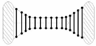
Figure 1: Two rod-like embedded (M- type) inclusions vertically inserted in a fluid biomembrane showing exponentially decaying thickness-matching constraints on the bilayer at the boundaries of the inclusions. Heavy solid lines represent amphiphilic molecules. Figure based on [6].

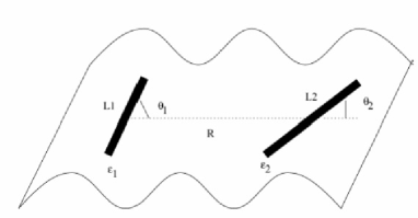
Figure 2: Two rod-like surface (S-type) inclusions placed on the surface of the biomembrane. The rods have lengths $L_{1}$ and $L_{2}$, widths $\epsilon_{1}$ and $\epsilon_{2}$ and making angles $\theta_{1}$ and $\theta_{2}$ with the line joining their centres of mass. Figure based on [32].

To implement the equations of motion, (24) and (25), we first required the computation of $D_{t}$. The computation of $D_{\bot}$ part of $D_{t}$ was based on (13) for a correlation time of $t=10^{-4}$s. Table I shows the variation of the $D_{\bot}$ for both the M-type and S-type inclusions for different values of the surface tension, $\sigma_{0}$. It can clearly be seen that the smaller is the surface tension, the larger is the value of the lateral diffusion constant.

T(K)	$\sigma_{0}$(J/$\mu$ m2)	D${}^{\tiny\mbox{M(S)}}_{\bot}$(m2s-1)
300	5$\times 10^{-23}$	0.25$\times 10^{-8}$
300	5$\times 10^{-21}$	0.71$\times 10^{-9}$
300	5$\times 10^{-18}$	0.46$\times 10^{-10}$

Table I: Computed values of the lateral diffusion constant for different values of surface tension.

To compute $D_{\|}$ on the basis of (15), we first performed a constant-temperature molecular dynamic (MD)-like calculation [29] in which the inclusions interacted with each other via the potentials given in (22) and (23). These potentials describe the M-M and S-S type interactions respectively. For the M-S interactions, we adopted the simple mixing rule of an arithmetic average of the M-M and S-S potentials. The temperature was kept constant at $T=300$ K by applying the Nosé-Hoover thermostat (heat bath) [33], and the simulation time-step was set at $dt=10^{-9}$s. During this simulation our aim was to obtain the positions of the inclusions as a function of simulation time, and these were recorded at specified time intervals, and the data were then used in (15) in a separate simulation code. The same correlation time, $t=10^{-4}$ s, that was used for the computation of $D_{\bot}$ was used for the computation of $D_{\|}$. In this case, this correlation time corresponded to the positions of inclusions recorded after $10^{5}$ time steps. The value of $D_{\|}$ for the M- and S-type inclusions corresponding to this delay time was obtained to be

$$D^{\tiny\mbox{M(S)}}_{\|}=0.99\times 10^{-11}\,\,\mbox{m${}^{2}$ s${}^{-1}$}.$$ (28)

Comparison of (28) and the values listed in Table I shows that the main contribution to the $D_{t}$ comes from the lateral component, which was also found to be comparable to the corresponding value of $D\approx 4.4\times 10^{-9}$ m²s^-1 obtained from an MD-based simulation of a fully hydrated phospholipid dipalmitoylphosphatidylcholine (DPPC) bilayer diffusing in the $z$-direction [34].

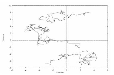
Figure 3: Stochastic trajectories of a sample of S-type inclusions. Both drift and diffusive motions are clearly visible.

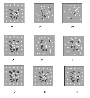
Figure 4: A series of snapshots from dynamic simulations showing the capture of the S-type inclusions (black spheres) at the cite of the M-type inclusions (white spheres) for dynamic M-type inclusions. The top row, (a)-(c), corresponds to the value of the surface tension $\sigma$=5$\times 10^{-23}$J/$\mu$m², the middle row, (d)-(f), to the value $\sigma$=5 $\times 10^{-21}$J/$\mu$m², and the bottom row, (g)-(i), to the value $\sigma$=5$\times 10^{-18}$J/$\mu$m². Only the centres of mass of the inclusions are shown.

The choice of correlation time, i.e. $t=10^{-4}$s, over which the values of the components of $D_{t}$ were computed has to be justified. We justify this choice by noticing that the diffusion time scale, $t_{D}$, for a stochastic particle of mass $m$ is given by [27]

$$t_{D}=\frac{mD}{k_{B}T}.$$ (29)

Since the relevant time scale for Brownian particles is at least, $t_{D}=10^{-9}$ s, then in order for the criterion of long-time dynamics, as embodied in (20), to be applicable to our model, the correlation time, $t$, in (13) and (15) over which the diffusion constants were calculated, must satisfy the condition [27]

$$t\gg t_{D}.$$ (30)

For the data given in (27) and the values of $D_{t}$ as computed from any of the relationships in given (18), the values of $t_{D}$ obtained from (29) turn out to be much smaller than $t$ indicating setting the value of the correlation time at $t=10^{-4}$ was quite reasonable.

A set of dynamic simulations, based on (24) and (25), were performed for the different combinations given in (18) to compute the stochastic trajectories for both the S-type and M-type inclusions, and the rate of capture of the S-type inclusions at the sites of the M-type inclusions. The temperature was set at $T$=300 K . The simulation time step, $dt$, in (24) and (25), was set at $dt=10^{-9}$ s, and each simulation was performed for a total time of 4000 $\mu$s, i.e. $4\times 10^{6}$ iterations. The total number of inclusions consisted of 13 S-type and 23 M-type. Table II shows the variation of the number of S-type inclusions captured at the site of M-type inclusions for different values of the surface tension and different combinations of $D_{t}$, with the values of $D_{\bot}$ and $D_{\|}$ given in Table I and (28). The data in this table refer to the capture of the S-type inclusions when both the S-type and the M-type inclusions were mobile.

Simulation data	$D_{t}=\frac{1}{2}(D_{\bot}+D_{\|})$	$D_{t}=\frac{1}{3}(2D_{\bot}+D_{\|})$	$D_{t}=\frac{1}{3}(D_{\bot}+2D_{\|})$
	captured S-type	captured S-type	captured S-type
$\sigma_{0}=5\times 10^{-23},\,\,T=300$	10	11	8
$\sigma_{0}=5\times 10^{-21},\,\,T=300$	3	4	3
$\sigma_{0}=5\times 10^{-18},\,\,T=300$	1	1	1

TableII: Variations of the number of captured S-type inclusions with surface tension and temperature for different different combinations of the lateral ($D_{\bot}$) and longitudinal ($D_{\|}$) diffusion coefficients. $\sigma_{0}$ is in units of J/$\mu$m², and the $D$s are in units of m² s^-1. Both the S-type and the M-type inclusions were mobile.

To make a comparison with the case when the M-type inclusions were static and only the S-type inclusions were mobile, the variation of the number of captured S-type inclusions for different combinations of $D_{t}$ was computed, and the results for a particular value of $\sigma_{0}$ are listed in Table III.

Simulation data	$D_{t}=\frac{1}{2}(D_{\bot}+D_{\|})$	$D_{t}=\frac{1}{3}(2D_{\bot}+D_{\|})$	$D_{t}=\frac{1}{3}(D_{\bot}+2D_{\|})$
	captured S-type	captured S-type	captured S-type
$\sigma_{0}=5\times 10^{-21},\,\,T=300$	3	3	2

Table III: Variations of the number of adsorbed S-type inclusions for different combinations of the lateral ($D_{\bot}$) and longitudinal ($D_{\|}$) diffusion coefficients when only the S-type inclusions were mobile.

Fig.3 shows the stochastic trajectories of a set of six S-type inclusions obtained from (24) and (25). Both drift motion, represented by the second term on the RHS of (24), and random diffusive, motion coming from membrane fluctuations, superimposed on the drift motion are visible.

Fig.4 shows the snapshots of a small portion of the biomembrane for a simulation in which both the M-type inclusions and the S-type inclusions were allowed to diffuse. In this figure, the black spheres represent the S-type inclusions and the white spheres the M-type inclusions. The spheres represent the centres of mass of the inclusions. The snapshots (a-c) refer to the case with $\sigma_{0}=5\times 10^{-23}$J/$\mu$m², (d-f) to the case with $\sigma_{0}=5\times 10^{-21}$J/$\mu$m², and (g-i) to the case with $\sigma_{0}=5\times 10^{-18}$J/$\mu$m². In each row of this figure, the first snapshot, e.g (a), refers to the initial state, the second snapshot, e.g. (b), to the state after 2000 $\mu$s and the last snapshot, e.g. (c), to the state after 4000 $\mu$s. In the initial state, e.g. (a), in this figure, the outer M-type inclusions were distributed regularly and the inner ones were distributed at random. For the S-type inclusions, these were all distributed completely at random. As can be clearly seen from the snapshots in Fig.4, the smaller the value of the surface tension, i.e. the top row snapshots, the higher the rate of capture of the S-type inclusions by the M-type inclusions. Furthermore, we observed that for the higher value of the surface tension, i.e. the bottom row, there was a clear collective motion of the S-type inclusions, i.e. the surface tension constrained the motion of the individual inclusions to an organised type of motion.

The bottom-row snapshots showed that neither type of inclusions made any significant diffusion during the simulation time, i.e. for this value of the surface tension, the stiffness of the patch practically prevented any appreciable movement of the inclusions. This implied that the biomembrane surface behaved in a more stiff manner than the case of low surface tension or the absence of surface tension as reported in [4]. The last snapshot in the first row of this figure shows that the majority of the S-type inclusions were captured by the M-type inclusions, and that there was a total disorder in the pattern of the M- type inclusions. This is similar to the results in our previous simulation in the absence of surface tension [4], although a bigger number of inclusions were captured during that simulation. This implies that as the surface tension becomes smaller and smaller, the biomembrane behaves more like a fluid, hence allowing an easier diffusion for any type of inclusions. This can have direct practical implications, namely, for the passage of external particles into the interior of a cell, the magnitude of the surface tension can play a very crucial role. A flexible biomembrane allows more external particles to arrive at the site of the embedded proteins (i.e. the M-type inclusions), hence increasing the rate of transport of material to the interior of the cell. This conclusion can have useful implications for the design artificial membranes, smart drugs and a better drug delivery mechanism.

To sum up, our computational simulation has been able to reveal the essential role played by the surface tension in the overall dynamics of the biomembrane. This is compatible with the experimental finding [21] in which it was found that for a surface tension value of $\sigma\geq 5\times 10^{-18}$J/$\mu$m² the vesicle becomes quite taut inducing an organised type of motion to the contents of the vesicle. In our previous simulation [4] it was shown that the rate of capture of the S-type inclusions was clearly affected by an increase in the temperature of the biomembrane. We can now add that this rate is also affected strongly by the presence of the surface tension in the biomembrane.

Another finding from our simulation is that the contribution of the lateral component of the diffusion coefficient, $D_{\bot}$, computed from the stochastic fluctuations of the height function of the biomembrane, far outweighs that of longitudinal coefficient, $D_{\|}$. In view of the fact that the larger is the value of the surface tension, the smaller the value of the diffusion coefficient becomes, then if the contribution of surface tension had also been included in the computation of the longitudinal component of the diffusion coefficient, this would have further reduced the value of this component and made its relative importance, vis-a-vise $D_{\bot}$, even less important.

References

- [1] J.H. Hunt, Foundations of Colloid Science, Clarendon Press, Oxford, 1993.
- [2] U. Seifert, Adv. in Phys. 46(1997)13.
- [3] S.J. Singer, G.L Nicolson, Science 175 (1972) 720.
- [4] H. Rafii-Tabar H and H.R. Sepangi, Comp.Mat. Sci. 15 (1999) 483.
- [5] N.Dan, P. Pincus, S.A. Safran, Langmuir 9 (1993) 2768.
- [6] N. Dan, A. Berman, P. Pincus, S.A. Safran, J. Phys. II France 4 (1994) 1713.
- [7] E.H. Mansfield, H.R. Sepangi, E.A. Eastwood, Phil. Trans. R. Soc. Lond. A 355 (1997) 869.
- [8] M.Bloom, E.Evans, O.G.Q Mouristen, Rev. Biophys. 24 (1991) 293.
- [9] J.R. Abney, J.C. Owicki, in : W. De Pont (Ed), Progress in Protein- Lipid Interactions, Elsevier, New York 1985.
- [10] S. Marcelja, Biophys. Acta 455 (1976)1.
- [11] J.C. Owicki, H.M. McConnell, Proc. Nat. Acad. Sci. USA 76(1979)4750.
- [12] D.R. Fattal. A. Ben- Shaul, Biophys. J. 65 (1993) 1795.
- [13] H.W. Huang, Biophys. J. 50 (1986) 1061.
- [14] D. Nelson, T. Piran and S. Weinberg, Statistical Mechanics of biomembranes and Surfaces, Jerusalem Winter School for Theoretical Physics, Vol 5, World Scientific, Singapore, 1989.
- [15] S.A. Safran, Statistical Thermodynamics of Surfaces, Interfaces and Biomembranes, Addison- Wesley, Reading, MA, 1994.
- [16] G.Gompper, M. Schick, Self-assembling Amphiphilic Systems, Phase Transition and Critical Phenomena, in : C. Domb, J. Lebowitz (Eds), Academic Press, London, 1994.
- [17] U. Seifert, Z. Phys. B 97 (1995) 299.
- [18] B. Alberts et al., Molecular Biology of the Cell, Garland, New York, 1994.
- [19] P. Sens, S.A. Safran, Europhys Lett. 43 (1998) 95.
- [20] E. Evans, W. Rawicz, Phys. Rev. Lett. 64 (1990) 2094.
- [21] R. Bar-Ziv, T. Frisch, E. Moses, Phys. Rev. Lett. 75 (1995) 3481; D. Moroz, P. Nelson, R. Bar-Ziv, E. Moses, Phys. Rev. Lett. 78 (1997) 386.
- [22] P.B. Canham, J. Theor. Biol. 26 (1970) 61.
- [23] W. Helfrich, Z. Naturforsh, 28c (1973) 693.
- [24] The Mathematica Version 5 (2003), Wolfram Research, Inc. Champaign Ill USA.
- [25] S.W. Chiu, M. Clark, V. Balaji, S. Subramaniam, H.L, Scott, E. Jakobsson, Biophys. J. 69 (1995) 1230.
- [26] J.M. Haile, Molecular Dynamics Simulation: Elementary Methods, Wiley, N.Y., 1992.
- [27] J.K.G. Dhont, An Introduction to Dynamics of Colloids, Elsevier, Amsterdam, 1996.
- [28] C.W. Gardiner, Handbook of Stochastic Methods, Springer, Berlin, 1990.
- [29] M.P Allen, D.J. Tildesley, Computer Simulation of Liquids, Clarendon Press, Oxford, 1987.
- [30] M. Goulian, R. Bruinsma Pincus P., Europhys.Lett. 22 (1993) 145.
- [31] M. Goulian, R. Bruinsma Pincus P., Europhys.Lett. 22 (1993) 155E.
- [32] R. Golestanian,M. Goulian, M. Kardar M., Europhys. Lett. 33 (1996) 241.
- [33] H. Rafii-Tabar , Phys. Rep. 325 (2000) 239.
- [34] D.P. Tieleman, H.J.C Berensden, J. Chem. Phys. 105 (1996) 4871.