Dendritic and uniform flux jumps in superconducting films

Abstract

Recent theoretical analysis of spatially-nonuniform modes of the thermomagnetic instability in superconductors slab is generalized to the case of a thin film in a perpendicular applied field. We solve the thermal diffusion and Maxwell equations taking into account nonlocal electrodynamics in the film and its thermal coupling to the substrate. The instability is found to develop in a nonuniform, fingering pattern if the background electric field, $E$, is high and the heat transfer coefficient to the substrate, $h_{0}$, is small. Otherwise, the instability develops in a uniform manner. We find the threshold magnetic field, $H_{\text{fing}}(E,h_{0})$, the characteristic finger width, and the instability build-up time. Thin films are found to be much more unstable than bulk superconductors, and have a stronger tendency for formation of fingering (dendritic) pattern.

I Introduction

The thermomagnetic instability or flux jumping is commonly observed at low temperatures in type-II superconductors with strong pinning. Mints81 ; Gurevich97 ; Wipf91 ; Wilson83 The instability arises for two fundamental reasons: (i) motion of magnetic flux releases energy, and hence increases the local temperature; (ii) the temperature rise decreases flux pinning, and hence facilitates the further flux motion. This positive feedback can result in thermal runaways and global flux redistributions jeopardizing superconducting devices. The conventional theory of the thermomagnetic instability Mints81 ; Gurevich97 considers only “uniform” flux jumps, where the flux front is smooth and essentially straight. This picture is true for many experimental conditions, however, far from all. Numerous magneto-optical studies have recently revealed that the thermomagnetic instability in superconductors can result in strongly branched dendritic flux patterns.Wertheimer67 ; Leiderer93 ; Bolz03 ; Duran95 ; welling ; Johansen02 ; Johansen01 ; Bobyl02 ; Barkov03 ; sust03 ; ye ; Rudnev03 ; jooss ; menghini ; Rudnev05

In a recent paper we examined the problem of flux pattern formation in the slab geometry. slab Experimentally, however, the dendritic flux patterns are mostly observed in thin film superconductors placed in a perpendicular magnetic field. A first analysis of this perpendicular geometry was recently published by Aranson et al.Aranson Here we present more exact and complete picture of the dendritic instability and analyze the criteria of its realization.

In the following we restrict ourselves to a conventional linear analysisMints81 ; Gurevich97 ; Wipf67 of the instability and consider the space-time development of small perturbations in the electric field, $E$, and temperature, $T$. In contrast to the slab case, slab the heat transfer from the superconductor to a substrate as well as the nonlocal electrodynamics in thin films are taken into account. Consequently, the results depend significantly on the heat transfer rate, $h_{0}$, as well as on the film thickness, $d$. Our main result is that the instability in the form of narrow fingers perpendicular to the background field, $\mathbf{E}$, occurs much easier in thin films than in slabs and bulk samples, and the corresponding threshold field, $E_{c}$, is found to be proportional to the film thickness, $d$.

II Model and basic equations

Consider the perpendicular geometry shown in Fig. 1, with a thin superconducting strip placed in a transverse magnetic field, $\mathbf{H}$. The strip is infinite along the $y$ axis, and occupies the space from $-d/2$ to $d/2$ in the $z$-direction and from $0$ to $2w$ in the $x$-direction. It is assumed that $d\ll w$. In the unperturbed state the screening current flows along the $y$-axis .

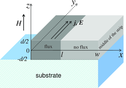
Figure 1: A superconductor strip on a substrate (only the left half is shown). The dark gray area is the flux-penetrated region.

The distributions of the current density, $\mathbf{j}$, and magnetic induction, $\mathbf{B}$, in the flux penetrated region $0<x<\ell$ are determined by the Maxwell equation

$$\textrm{curl }\mathbf{B}=\mu_{0}\mathbf{j}\,,$$ (1)

where the common approximation $\mathbf{B}=\mu_{0}\mathbf{H}$ is used. To find the electric field and the temperature we use another Maxwell equation together with the equation for thermal diffusion,

$$\textrm{curl }\mathbf{E} = -\partial\mathbf{B}/\partial t\,,$$ (2)

$$C(\partial T/\partial t) = \kappa\nabla^{2}T+\mathbf{j}\mathbf{E}\,.$$ (3)

Here $C$ and $\kappa$ are the specific heat and thermal conductivity, respectively.

Equations (1)-(3) should be supplemented by a current-voltage relation $j=j(E,B,T)$. For simplicity we assume a current-voltage curve of the form

$$\mathbf{j}=j_{c}(T)g(E)\,(\mathbf{E}/E)\,.$$ (4)

A strong nonlinearity of the function $g(E)$ leads to formation of a quasi-static critical state with $j\approx j_{c}(T)$, where $j_{c}$ is the critical current density.Bean We neglect any $B$-dependence of $j_{c}$, i. e., adopt the Bean model. The exact form of $g(E)$ is not crucially important, the only issue is that it represents a very steep $E(j)$ curve having a large logarithmic derivative,

$$n(E)\equiv\partial\ln E/\partial\ln j\approx j_{c}/\sigma E\gg 1\,.$$ (5)

Here $\sigma$ is the differential electrical conductivity, $\sigma(E)\equiv\partial j/\partial E$. The parameter $n$ generalizes the exponent in the frequently used power-law relation $E\propto j^{n}$ with $n$ independent of $E$.

The key dimensionless parameter of the model is the ratio of thermal and magnetic diffusion coefficients,Mints81

$$\tau\equiv\mu_{0}\kappa\sigma/C\,.$$ (6)

The smaller $\tau$ is, the slower heat diffuses from the perturbation region into the surrounding areas. Hence, one can expect that for smaller $\tau$: (i) the superconductor is more unstable, and (ii) the formation of instability-induced nonuniform structures is more favorable.

In the following we assume that the strip is thinner than the London penetration depth, $\lambda_{L}$, and at the same time much wider than the effective penetration length, $\lambda_{\text{eff}}=\lambda^{2}_{L}/d$,

$$d\leq\lambda_{L}\ll\sqrt{dw}\,.$$

The stationary current and field distributions in a thin strip under such conditions were calculated by several authors, Norris70 ; BrIn ; zeld finding that the flux penetration depth, $\ell$, is related to the applied field by the expression

$$\ell\,/\,w\,=\,\pi^{2}H^{2}/2d^{2}j_{c}^{2}\ .$$ (7)

Here it is assumed that the penetration is shallow, or more precisely that $\lambda_{\text{eff}}\ll\ell\ll w$.

III Perturbation analysis

III.1 Linearized dimensionless equations

We seek solutions of Eqs. (1)-(4) in the form

$$T+\delta T(x,y,z,t),\quad\mathbf{E}+\delta\mathbf{E}(x,y,z,t),\quad\mathbf{j}+\delta\mathbf{j}(x,y,z,t)$$

where $T$, $\mathbf{E}$ and $\mathbf{j}$ are background values. The background electric field may be created, e. g., by ramping the external magnetic field, and for simplicity we assume it to be coordinate independent. Allowing for such a dependence would only lead to insignificant numerical corrections, as discussed in Ref. slab, . Similarly, we will assume a uniform background temperature.

Whereas it follows from symmetry considerations that $E_{x}=0$, both components of the perturbation, $\delta\mathbf{E}$, will in general not vanish. Linearizing the current-voltage relation, Eq. (4) one obtains:

$$\delta\mathbf{j}=\left(\frac{\partial j_{c}}{\partial T}\,\delta T+\sigma\,\delta E_{y}\right)\frac{\mathbf{E}}{E}+j_{c}\frac{\delta\mathbf{E}_{x}}{E}\,.$$ (8)

We shall seek perturbations in the form

$$\delta T = T^{*}\theta\exp(\lambda t/t_{0}+ik_{x}\xi+ik_{y}\eta)\,,$$

$$\delta E_{x,y} = E\varepsilon_{x,y}\exp(\lambda t/t_{0}+ik_{x}\xi+ik_{y}\eta)\,,$$

$$\delta j_{x,y} = j_{c}i_{x,y}\exp(\lambda t/t_{0}+ik_{x}\xi+ik_{y}\eta)\,,$$ (9)

where $\theta$, $\varepsilon$ and $i$ are $z$-dependent dimensionless Fourier amplitudes. The coordinates are normalized to the adiabatic length $a=\sqrt{CT^{*}/\mu_{0}j_{c}^{2}}$ where $T^{*}=-(\partial\ln j_{c}/\partial T)^{-1}$ is the characteristic scale of the temperature dependence of $j_{c}$, so that $\xi=x/a$, $\eta=y/a$, $\zeta=z/a$. The time is normalized to $t_{0}=\sigma CT^{*}/j_{c}^{2}=\mu_{0}\sigma a^{2}$, which is the magnetic diffusion time for the length $a$. $\mathop{\mathrm{Re}}\lambda$ is the dimensionless instability increment, which when positive indicates exponential growth of the perturbation.

We can now use the formulas (9) to rewrite the basic equations in dimensionless variables. From Eq. (8) one finds for the components of the current density perturbation $\mathbf{i}$,

$$i_{x}=\varepsilon_{x}\,,\quad i_{y}=-\theta+n^{-1}\varepsilon_{y}\,.$$ (10)

Combining the Maxwell equations  (1) and (2), and the thermal diffusion equation (3) yields

$${\bf k}\times[{\bf k}\times\mathbf{\varepsilon}]=\lambda n\,\mathbf{i}\,,$$ (11)

$$\lambda\theta=\tau\left(-k_{y}^{2}\theta+\frac{\partial^{2}\theta}{\partial\zeta^{2}}\right)+(i_{y}+\varepsilon_{y})/n\,.$$ (12)

Magneto-optical imaging shows that flux patterns produced by the dendritic instabilityWertheimer67 ; Leiderer93 ; Bolz03 ; Duran95 ; welling ; Johansen02 ; Johansen01 ; Bobyl02 ; Barkov03 ; sust03 ; ye ; Rudnev03 ; jooss ; menghini ; Rudnev05 are characterized by having $k_{y}\gg k_{x}$. Therefore, we have neglected the heat flow along $x$ direction compared to that along the $y$ direction. Later we will check the consistency of this assumption by showing that indeed the fastest growing perturbation has $k_{y}\gg k_{x}$.

III.2 Boundary conditions

We assume that heat exchange between the superconducting film and its environment follows the Newton cooling law. For simplicity we let the boundary condition, $\kappa\nabla(T+\delta T)=-h_{0}(T+\delta T-T_{0})$, apply to both film surfaces. Here $T_{0}$ and $h_{0}$ are the effective environment temperature and heat transfer coefficient, respectively. Eqs. (12) and  (10) can now be integrated over the film thickness to yield

$$\theta=\frac{(1+n^{-1})\varepsilon_{y}}{n\lambda+n\tau(k_{y}^{2}+h)+1}$$

where

$$h=2h_{0}a^{2}/\kappa d\,.$$ (13)

In the remaining part of the paper we let $\theta$, $\mathbf{\varepsilon}$ and $\mathbf{i}$ denote perturbations averaged over the film thickness.

We seek a solution of the electrodynamic equations in the flux penetrated region, $0\leq\xi\leq\ell/a$. At the film edge, $\xi=0$, one has $\delta j_{x}=0$ and, consequently, $\delta E_{x}=0$. In the Meissner state both the electric field and heat dissipation are absent, so that $\delta E_{y}=\delta T=\delta j_{y}=0$ at the flux front, $\xi=\ell/a$. Thus, the Fourier expansions for the $x$ and $y$ components of electric field perturbation will contain only $\sin(k_{x}\xi)$ and $\cos(k_{x}\xi)$, respectively. Then the boundary conditions are satisfied for

$$k_{x}=\left(\pi a/2\ell\right)(2s+1)\,,\quad s=0,1,2,\ldots\,.$$

Since $\ell$ depends on magnetic field, the values of $k_{x}$ are also magnetic field dependent.

Now we can integrate Eq. (11) over the film thickness and employ the symmetry of the electrodynamic problem with respect to the plane $z=0$. It yields

$$-ik_{y}(k_{x}\varepsilon_{y}+ik_{y}\varepsilon_{x})-\frac{2a}{d}\varepsilon_{x}^{\prime} = -\lambda n\varepsilon_{x},$$

$$-k_{x}(k_{x}\varepsilon_{y}+ik_{y}\varepsilon_{x})+\frac{2a}{d}\varepsilon_{y}^{\prime} = -\lambda nf(\lambda,k_{y})\varepsilon_{y}\,.$$ (14)

We have here introduced the function

$$f(\lambda,k_{y})\equiv\frac{i_{y}}{\varepsilon_{y}}\frac{1}{n}-\frac{1+n^{-1}}{n\lambda+n\tau(k_{y}^{2}+h)+1}\,.$$

Note that the equation for the $z$-component of the field is satisfied automatically. The derivatives $\varepsilon_{x,y}^{\prime}$ with respect to $\zeta$ are taken at the film surface, $\zeta=d/2a$. To calculate them, one needs the electric field distribution outside the superconductor, where the flux density is given by the Bio-Savart law,

$$\mathbf{B(\mathbf{r})}=\mu_{0}\mathbf{H}+\frac{\mu_{0}}{4\pi}\int d^{3}\mathbf{r^{\prime}}\,\frac{\mathbf{j}\times(\mathbf{r}-\mathbf{r^{\prime}})}{|\mathbf{r}-\mathbf{r^{\prime}}|^{3}}\,.$$

The perturbation of flux density is then,

$$\delta B_{x,y}=\pm\mu_{0}\zeta d\int^{\ell/a}_{0}d\xi^{\prime}\int^{\infty}_{-\infty}d\eta^{\prime}G(\xi-\xi^{\prime},\eta-\eta^{\prime})\delta j_{y,x},$$

$$\quad G(\xi,\eta)=\frac{1}{4\pi\left(\xi^{2}+\eta^{2}+(d/2a)^{2}\right)^{3/2}}.$$ (15)

Here we have approximated the average over $\zeta^{\prime}$ substituting $\zeta^{\prime}=0$. In this way we omit only terms of the order of $(d/a)^{2}\ll 1$. The integration over $\xi^{\prime}$ should, in principle, cover also the Meissner region, $\xi^{\prime}>l/a$. Though the flux density there remains zero during the development of perturbation, the Meissner current will be perturbed due to the nonlocal current-field relation. However the kernel $G(\xi,\eta)$ decays very fast at distances larger than $d/a$ and therefore the Meissner current perturbation produces only insignificant numerical corrections.

The perturbation of magnetic field can be related to that of electrical field by Eq. (2), which can be rewritten as

$$\delta E^{\prime}_{x,y}/E=\mp\lambda n\,\delta B_{y,x}/\mu_{0}aj_{c}\,.$$ (16)

Due to continuity of the magnetic field tangential components Eq. (16) is also valid at the film surface, $\zeta=d/2a$. Thus it can be substituted into Eqs. (14). The Fourier components of the kernel function $G(\xi,\eta)$ with respect to $\eta$ can be calculated directly yielding

$$G(\xi,k_{y})=\frac{k_{y}a}{2\pi\ell}\cdot\frac{\mathrm{K}_{1}\left(k_{y}\sqrt{\xi^{2}+(d/2a)^{2}}\right)}{\sqrt{\xi^{2}+(d/2a)^{2}}}$$ (17)

where $K_{1}$ is the modified Bessel function of the second kind.

The above Fourier expansions in $\cos(k_{x}\xi)$ and $\sin(k_{x}\xi)$ correspond to the finite interval $-2\ell/a<\xi<2\ell/a$. Therefore we should continue $\varepsilon_{x,y}$ from $0<\xi<\ell/a$ to this interval and then introduce $G_{x}$ and $G_{y}$ as analytical continuations of $G(\xi-\xi^{\prime},k_{y})$ having the same symmetry as $\varepsilon_{x}$ and $\varepsilon_{y}$, respectively (see Section VI for details). All this allows us to rewrite the set (14) as

$$-ik_{x}k_{y}\varepsilon_{y}+(k_{y}^{2}+\lambda n)\varepsilon_{x}$$

$$\qquad=(d/2a)\lambda n\sum_{k_{x}^{\prime}}G_{x}(k_{x},k_{x}^{\prime},k_{y})\varepsilon_{x}(k_{x}^{\prime})\,,$$ (18)

$$(k_{x}^{2}+\lambda nf)\varepsilon_{y}+ik_{x}k_{y}\varepsilon_{x}$$

$$\qquad=(d/2a)\lambda nf\sum_{k_{x}^{\prime}}G_{y}(k_{x},k_{x}^{\prime},k_{y})\varepsilon_{y}(k_{x}^{\prime})\,,$$ (19)

$$\left\{\begin{array}[]{c}G_{x}(k_{x},k_{x}^{\prime},k_{y})\\ G_{y}(k_{x},k_{x}^{\prime},k_{y})\end{array}\right\}=4\int^{\ell/a}_{0}\!\!\!\!d\xi\int^{\ell/a}_{0}\!\!\!\!d\xi^{\prime}G(\xi-\xi^{\prime},k_{y})$$ (22)

$$\qquad\times\left\{\begin{array}[]{c}\sin(k_{x}\xi)\sin(k_{x}^{\prime}\xi^{\prime})\\ \cos(k_{x}\xi)\cos(k_{x}^{\prime}\xi^{\prime})\end{array}\right\}\,.$$ (25)

We are interested only in the specific case of very thin strip,

$$\alpha=d/2\ell\ll 1\,.$$ (26)

One can then find analytical expressions for the kernel, and it turns out that only its diagonal part, $k_{x}=k_{x}^{\prime}$, is important.

In this manuscript we present analytical expressions up to the first order in $\alpha$, while the plots are calculated up to the second order. The second-order analytical expressions can be found in section VI. The kernel (25) can be written as

$$G_{x,y}(k_{x},k_{x},k_{y})=\frac{a}{\ell}\left[\frac{1-\gamma(\alpha,k_{x})\alpha}{\alpha}\right],$$ (27)

where $\gamma(\alpha,k_{x})$ is a dimensionless function. In what follows we shall consider only the main instability mode, $k_{x}=\pi a/2\ell$, which turns out always to be the most unstable one. For this mode, and in the limit $\alpha\to 0$, the function $\gamma(\alpha,k_{x})$ approaches a constant value $\approx 5$.

Substituting the above expression for $G$ into Eqs. (18) and (19) one obtains the dispersion relation for $\lambda(k_{x},k_{y})$:

$$A_{1}\lambda^{2}+A_{2}\lambda+A_{3}=0\,.$$ (28)

Here

$$A_{1}=n\gamma\alpha\,,\quad A_{2}=k_{y}^{2}(1+\tau A_{1})+nk_{x}^{2}+A_{1}(h\tau-1)\,,$$

$$A_{3}=k_{y}^{4}\tau+nk_{x}^{2}k_{y}^{2}\tau+nk_{x}^{2}(h\tau+1/n)+k_{y}^{2}(h\tau-1).$$

IV Results

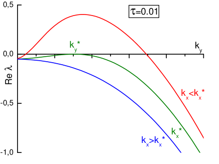
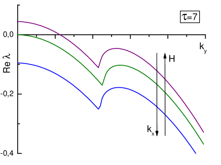
Figure 2: Solutions of dispersion equation (28) for small and large $\tau$, for $\alpha=0.001$ and n=20.

Let us first consider the simple case of a uniform perturbation, $k_{y}=0$. One finds from Eq. (28) that the perturbation will grow ($\mathop{\mathrm{Re}}\lambda>0$) if

$$h\tau<1-k_{x}^{2}/\gamma\alpha\,.$$ (29)

When the flux penetration region, $\ell$, is small, i. e., $k_{x}$ is large, the system is stable. As the flux advances, $k_{x}$ decreases, and the system can eventually become unstable. The instability will take place, however, only if $h\tau<1$. Otherwise the superconducting strip of any width will remain stable no matter how large magnetic field is applied. This size-independent stability means that at $h\tau\geq 1$ the heat dissipation due to flux motion is slower than heat removal into the substrate.

Equation (29) further simplifies in the adiabatic limit, $\tau\to 0$, when the heat production is much faster than heat diffusion within the film or into the substrate. The instability then develops at $k_{x}^{2}/(\gamma\alpha)<1$, which in dimensional variables reads as $\mu_{0}j_{c}^{2}ld>CT^{*}(\pi^{2}/2\gamma)$. Assuming small penetration depth, $l\ll w$, and using Eq. (7) this criterion can be rewritten as $H>H_{\text{adiab}}$, with the adiabatic instability field,

$$H_{\text{adiab}}=\sqrt{\frac{d}{w}\ \frac{CT^{*}}{\gamma\mu_{0}}}\sim\sqrt{\frac{d}{w}}\,\ H_{\text{adiab}}^{\text{slab}}\,.$$ (30)

Here $H_{\text{adiab}}^{\text{slab}}$ is the adiabatic instability field for the slab geometry.Mints81 ; Gurevich97 ; Wipf91 ; Wilson83 ; Wipf67 This result coincides up to a numerical factor with the adiabatic instability field for a thin strip found recently in Ref. Shantsev05, .

Solutions of Eq. (28) for perturbations with arbitrary $k_{y}$ are presented in Fig. 2. The upper panel shows $\mathop{\mathrm{Re}}\lambda(k_{y})$ curves for $\tau=0.01$ and different values of $k_{x}$. For large $k_{x}$, i. e., small magnetic field, $\mathop{\mathrm{Re}}\lambda$ is negative for all $k_{y}$. It means that the superconductor is stable. However, at small $k_{x}$, the increment $\mathop{\mathrm{Re}}\lambda$ becomes positive in some finite range of $k_{y}$. Hence, some perturbations with a spatial structure will start growing. They will have the form of fingers of elevated $T$ and $E$ directed perpendicularly to the flux front. We will call this situation the fingering (or dendritic) instability.

For large $\tau$ an instability also develops at small $k_{x}$, however in a different manner, see Fig. 2 (lower panel). Here the maximal $\mathop{\mathrm{Re}}\lambda$ always corresponds to $k_{y}=0$. Hence, the uniform perturbation will be dominant. The uniform growth of perturbations for large $\tau$ has been recently predicted in Refs. slab, ; Aranson, and explained by the prevailing role of heat diffusion.

Let us now find the critical $k_{y}^{*}$ and $k_{x}^{*}$ for the fingering instability, see Fig. 2 (upper panel). The $k_{x}^{*}$ determines the applied magnetic field when the instability first takes place, while $k_{y}^{*}$ determines its spatial scale. These quantities can be found from the requirement $\max\{\mathop{\mathrm{Re}}\lambda(k_{y})\}=0$ for $k_{y}\neq 0$. In the limit $\alpha\ll 1$ we can put $A_{1}=0$ in Eq. (28) and then rewrite it in the form

$$\lambda=-(k_{y}^{2}+h)\tau+\frac{(k_{y}^{2}-k_{x}^{2})}{k_{y}^{2}+nk_{x}^{2}}\,.$$

From this expression we obtain

$$k_{x}^{*} = \left(\sqrt{n+1}-\sqrt{nh\tau}\right)/n\sqrt{\tau}\,,$$ (31)

$$k_{y}^{*} = \left[\sqrt{nh\tau+1}\left(\sqrt{n+1}-\sqrt{nh\tau+1}\right)\right]^{1/2}/\sqrt{n\tau}\,.$$

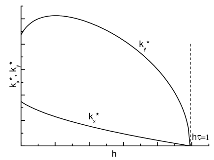
Figure 3: Dependences of $k_{y}^{*}$ and $k_{x}^{*}$ on $h$ for n=20, $\tau=0.01$, $\alpha=0.001$ according to Eq. (31).

The dependences of $k_{x}^{*}$, $k_{y}^{*}$ on the heat transfer coefficient $h$ are shown in Fig. 3. One can see that $k_{y}^{*}$ is always larger than $k_{x}^{*}$ implying that fingers of elevated $T$ and $E$ are extended in the direction normal to the film edge. For $h\ll 1/\tau$ and $n\gg 1$ we find $k_{y}^{*}\approx n^{1/4}k_{x}^{*}\gg k_{x}^{*}\approx 1/\sqrt{n\tau}$. Both $k_{x}^{*}$ and $k_{y}^{*}$ tend to zero as $h\to 1/\tau$, while for larger $h$ the system is always stable due to fast heat removal to the substrate.

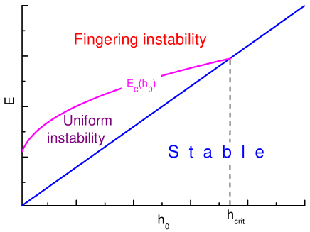
Figure 4: Stability diagram in the plane electric field – heat transfer coefficient according to equation Eq. (33) and condition $1-h\tau>0$ for $n=30$ and $\alpha=0.001$.

It follows from Fig. 2 that for large enough $\tau$ the instability will develop uniformly, while for small $\tau$ it will acquire a spatially-nonuniform structure. Let us find now the critical value $\tau_{c}$ that separates these two regimes. It can be obtained from the equality $\mathop{\mathrm{Re}}\lambda(k_{x}=k_{x}^{*},k_{y}=0)=0$. When it is fulfilled $\mathop{\mathrm{Re}}\lambda=0$ both for $k_{y}=0$ and for $k_{y}=k_{y}^{*}\neq 0$. We find using Eq. (28) that the instability will evolve in a spatially-nonuniform way if

$$\tau<\tau_{c}=\left(1-k_{x}^{*2}/\gamma\alpha\right)/h\,.$$ (32)

Substituting here $\alpha$ and $k_{x}^{*}$ we find a transcendental relation between $\tau_{c}$ and $h$. For $n\gg 1$ it reduces to

$$\sqrt{n\tau_{c}}\left(1+\sqrt{h\tau_{c}}\right)=\pi a/\gamma d\,.$$ (33)

Using this result we can construct a stability diagram in the $E-h_{0}$ plane shown in Fig. 4. The curved line marks the critical electric field $E_{c}(h_{0})$ that separates two types of instability: fingering ($E>E_{c}$) and uniform ($E<E_{c}$). This line is calculated from Eq. (33), where the electric field is expressed via $\tau$ as $E=j_{c}\mu_{0}\kappa/nC\tau$ according to Eqs. (5) and (6). The straight line is given by the condition $h\tau=1$. Below this line the superconductor is always stable, as follows from Eq. (29) for the uniform perturbations, and from Eq. (31) for the nonuniform case. At a certain value $h_{0}=h_{\text{crit}}$, the two lines intercept. We find

$$h_{\text{crit}}=\frac{2\gamma^{2}\mu_{0}^{2}j_{c}^{4}d^{3}\kappa n}{\pi^{2}T^{*2}C^{2}}\,,$$ (34)

and the critical electric field $E_{c}$ for $h_{0}=0$ is

$$E_{c}(0)=\frac{\gamma^{2}\mu_{0}^{2}\kappa j_{c}^{3}}{\pi^{2}C^{2}T^{*}}\ d^{2}\ ,$$ (35)

while $E_{c}(h_{\text{crit}})=4E_{c}(0)$.

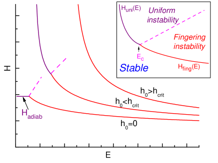
Figure 5: Stability diagram in the $H$-$E$ plane according to Eq. (29) and Eq. (31).

For any point ($h_{0}$,$E$) belonging to the stable phase in the stability diagram, Fig. 4, the flux distribution is stable for any applied magnetic field. For the points belonging to unstable phases, the instability develops above some threshold magnetic field, either $H_{\text{fing}}(h_{0},E)$ or $H_{\text{uni}}(h_{0},E)$ for fingering or uniform instability, respectively. Shown in Fig. 5 are three sets of $H_{\text{fing}}(E)$ and $H_{\text{uni}}(E)$ curves for different values of $h_{0}$. They represent boundaries between the three phases, stable and unstable with respect to either fingering or uniform instability, as shown in the inset. Using Eq. (7) one can rewrite the expression Eq. (29) for $H_{\text{uni}}$ as

$$H_{\text{uni}}=H_{\text{adiab}}\left(1-\frac{2T^{*}h_{0}}{nd\,j_{c}E}\right)^{-1/2}\,.$$ (36)

In the absence of heat removal to the substrate, $h_{0}=0$, we obtain the adiabatic instability field, Eq. (30), and the $H_{\text{uni}}(E)$ curve becomes a horizontal line.heatx

The threshold magnetic field for the fingering instability, $H_{\text{fing}}$, is calculated from Eq. (31). A simplified expression obtained for $h\ll 1/\tau$ and $n\gg 1$,

$$H_{\text{fing}}=\left(\frac{j_{c}d^{2}}{\pi w}\sqrt{\frac{\kappa T^{*}j_{c}}{E}}\right)^{1/2}\,,$$ (37)

shows that at large electric fields $H_{\text{fing}}$ decays as $E^{-1/4}$. At $h_{0}\leq h_{\text{crit}}$ the curves $H_{\text{fing}}(E)$ and $H_{\text{uni}}(E)$ intercept at the critical electric field $E_{c}$ determined by Eq. (32). At $h_{0}\geq h_{\text{crit}}$ we have $H_{\text{fing}}(E)<H_{\text{uni}}(E)$ for any $E$, so the lines do not intercept and the instability will develop into a fingering pattern.

V Discussion

Let us compare the present results for a thin film in a perpendicular magnetic field with results of Ref. slab, for a bulk superconductor. In both cases the instability develops into a fingering pattern if the background electric field in the superconductor exceeds some critical value $E_{c}$. The values of $E_{c}$ are however different. Their ratio for a thin strip and a slab,

$$\frac{E_{c}(0)}{E_{c}^{\text{slab}}}=\frac{\gamma^{2}}{\pi^{2}}\ \frac{d^{2}j_{c}^{2}\mu_{0}}{CT^{*}}\,,$$ (38)

is expected to be much less than unity. For $j_{c}=10^{10}$ A/m², $C=10^{3}$ J/Km³, $\kappa=10^{-2}$ W/Km, $T^{*}=10$ K and $d=0.3\,\mu$m, we find from Eq. (35) that $E_{c}\approx 4\cdot 10^{-4}$ V/m, while according to Ref. slab, , $E_{c}^{\text{slab}}=0.1$ V/m. Consequently, the development of thermomagnetic instability into a fingering pattern is much more probable in thin films than in bulk superconductors.

The threshold magnetic field for the fingering instability, $H_{\text{fing}}$, is also much smaller for thin films. Comparing Eq. (37) with the results of Ref. slab, for a slabslab we find

$$\frac{H_{\text{fing}}}{H_{\text{inst}}^{\text{slab}}}=\frac{\sqrt{2}}{\pi}\frac{d}{\sqrt{wl^{*}}}\,.$$ (39)

Here $l^{*}=(\pi/2)\sqrt{\kappa T^{*}/j_{c}E}$ is the flux penetration depth at the threshold of the fingering instability, $H=H_{\text{fing}}$. Experimentally, the fingering instability always starts after the flux has penetrated a noticeable distance from the edges, such that $l^{*}\gg d$.Wertheimer67 ; Leiderer93 ; Bolz03 ; Duran95 ; welling ; Johansen02 ; Johansen01 ; Bobyl02 ; Barkov03 ; sust03 ; ye ; Rudnev03 ; jooss ; menghini ; Rudnev05 Hence, for a thin film the fingering instability should start at much smaller applied fields than in bulk samples (by a factor of $\sim 10^{3}$ for films with $d\sim 10^{-4}w$). The difference between the threshold fields for the two geometries here is even stronger than for the case of uniform instability in the adiabatic limit, see Eq. (30). Assuming the above values of parameters and $w=2$ mm we find from Eq. (37) that $H_{\text{fing}}[E_{c}(0)]=H_{\text{adiab}}\approx 1$ mT. This value becomes larger if we take into account the heat transfer to the substrate. It is therefore in excellent agreement with experiment,Duran95 ; welling ; Johansen02 ; Barkov03 ; Rudnev03 ; jooss ; Rudnev05 ; Shantsev05 where the threshold field is typically of the order of a few milliTesla.

The spatial structure of the instability predicted by our linear analysis is a periodic array of fingers perpendicular to the film edge. Its period can be estimated from Eq. (31). For $E=E_{c}$, $h=0$ and $n\gg 1$ one finds

$$d_{y}=\frac{\pi^{2}CT^{*}}{2\gamma n^{1/4}\mu_{0}j_{c}^{2}d}\,,$$ (40)

which yields $d_{y}\approx 100\ \mu$m for $n=30$. Numerical analysis of the instability development showsAranson ; slab that beyond the linear regime the periodic structure is destroyed and only one (strongest) finger invades the Meissner region. This scenario is indeed reproduced experimentally, and the observed width of individual fingers, 20-50 $\mu$m,Leiderer93 ; Duran95 ; Johansen01 ; Barkov03 is very close to our estimate, $d_{y}/2$.

The finger width and the threshold magnetic field also depend on the dimensionless parameter $h$ characterizing the thermal coupling to the substrate, Eq. (13). In turn, $h$, grows rapidly with temperature because of a strong $T$ dependence of $C$ and $j_{c}$. One can therefore make several testable predictions from the dependences $k_{x}^{*}(h)$ and $k_{y}^{*}(h)$ shown in Fig. 3: (i) There must be a threshold temperature $T_{\text{th}}$ above which the instability is not observed. (ii) When approaching $T_{\text{th}}$, the instability field diverges since $k_{x}^{*}\to 0$. (iii) When approaching $T_{\text{th}}$ the characteristic width of individual fingers increases since $k_{y}^{*}\to 0$. The last prediction has also been obtained in the boundary layer model allowing calculation of the exact finger shape.Baggio The first and the second predictions have already been confirmed experimentally.Johansen01 ; welling As for the last one, the $T$ dependence of the finger width has not yet been studied. At the same time, there is a solid experimental evidenceDuran95 ; Johansen01 ; welling ; Rudnev05 for an enhanced degree of branching as $T\to T_{\text{th}}$ that can be quantitatively described as a larger fractal dimension of the flux pattern.Rudnev05 This abundant branching could be an indirect consequence of the increased finger width since wider fingers are presumably more likely to undergo splitting.

The present problem of fingering instability in a thin film has two new features compared to a similar problem for a bulk superconductor, (i) nonlocal electrodynamics and (ii) thermal coupling to the substrate. The nonlocality results in much smaller values of the threshold magnetic field $H_{\text{fing}}$ and the critical electric field $E_{c}$ in films than in bulks. If a film is made thinner, it becomes even more unstable since $H_{\text{fing}}\propto d$, and has a stronger tendency to form a fingering pattern since $E_{c}(0)\propto d^{2}$. The thermal coupling to the substrate has a somewhat opposite effect. It can lead to an ultimate stability if $h>1/\tau$ – a situation that is never realized in bulks. A moderate coupling, $h\ll 1/\tau$, slightly renormalizes $H_{\text{fing}}$ and $E_{c}$, i.e. makes the film a little bit more stable and less inclined to fingering.

Let us now compare the results presented in this work to those obtained in a similar model by Aranson et al.Aranson Our expressions for the “fingering” threshold field , Eq. (37), and for the finger width, Eq. (40), agree with their results up to a numerical factor. For $\tau\gg 1$ our results for the “uniform” threshold field (derived from Eq. (29)) are also similar to results of Ref. Aranson, . As a new result, we find that there exists a critical value of the parameter $\tau$, Eq. (32), which controls whether the instability evolves either in the uniform, or in the fingering way. Shown in Fig. 4 is the stability diagram where the line $E_{c}(h_{0})$ separates regimes of fingering and uniform instability. Other new results of this paper are: (i) the existence of a field-independent “critical point”, $h_{\text{crit}}$, such that for $h_{0}>h_{\text{crit}}$ the instability always develops into a fingering pattern, and (ii) the full stability diagram in the $H$-$E$ plane, Fig. 5, containing all three phases.

The background electric field needed to nucleate the fingering instability can be induced by ramping the magnetic field, $E\sim\dot{H}l\propto\dot{H}H^{2}$ for $l\ll w$, where $\dot{H}$ is the ramp rate. This is the lowest estimate since the flux penetration in practice is strongly nonuniform in space and in time,AltRev and there can be additional sources of $E$ due to random fluctuations of superconducting parameters. The occurrence of the fingering instability even at rather low ramp rates Wertheimer67 ; Duran95 ; welling ; Johansen02 ; Barkov03 ; Rudnev03 ; jooss ; menghini ; Rudnev05 is therefore not surprising.

The build-up time of the instability can be estimated as $t_{0}\approx 0.1\mu$s  if the flux-flow conductivity $\sigma=10^{9}\ \Omega^{-1}m^{-1}$. Our linear analysis assumes that the perturbations of $T$ and $E$ grow in amplitude, but remain localized within the initial flux penetrated region. Numerical results showslab ; Aranson that at $t\gg t_{0}$ the perturbations also propagate into the Meissner region. This propagation can be described by recent modelsbiehler05 ; shapiro that predict a characteristic propagation speed in agreement with experimental values of 10-100 km/s.Leiderer93 ; Bolz03

In conclusion, the linear analysis of thermal diffusion and Maxwell equations shows that a thermomagnetic instability in a superconducting film may result in either uniform or finger-like distributions of $T$, $E$ and $B$. The fingering distributions will be observed if the background electric field $E>E_{c}$, where $E_{c}$ grows with the film thickness, the critical current density, the thermal conductivity and the thermal coupling to the substrate. Due to nonlocal electrodynamics in thin films they turn out to be more unstable than bulk superconductors and more susceptible to formation of a fingering pattern.

VI Appendix

Here we present in more detail some derivations omitted in main text.

VI.1 Eq. (11)

In components, equation (11) reads as

$$ik_{y}\left(\frac{\partial\varepsilon_{y}}{\partial\xi}-ik_{y}\varepsilon_{x}\right)-\frac{\partial^{2}\varepsilon_{x}}{\partial\zeta^{2}} = -\lambda n\varepsilon_{x}\,,$$ (41)

$$\frac{\partial}{\partial\xi}\left(\frac{\partial\varepsilon_{y}}{\partial\xi}-ik_{y}\varepsilon_{x}\right)+\frac{\partial^{2}\varepsilon_{y}}{\partial\zeta^{2}} = \lambda nf(\lambda,k_{y})\varepsilon_{y}\,,$$ (42)

$$\frac{\partial}{\partial\zeta}\left(\frac{\partial\varepsilon_{x}}{\partial\xi}+ik_{y}\varepsilon_{y}\right) = 0\,.$$ (43)

VI.2 Transition from Eq.(17) to Eq.(25)

The Fourier transformation for the kernel function $G$ with respect to variable $\eta$ reads

$$G(\xi,\eta,\alpha) = \int^{\infty}_{-\infty}\frac{dk_{y}}{2\pi}G(\xi,k_{y},\alpha)e^{ik_{y}\eta}\,,$$ (44)

$$G(\xi,k_{y},\alpha) = \int^{\infty}_{-\infty}d\eta G(\xi,\eta,\alpha)e^{-ik_{y}\eta}\,,$$ (45)

Substituting Fourier transformation of kernel $G$ into Eqs. (15) and (16), we find

$$\varepsilon^{\prime}_{x}(\xi,k_{y})=2\alpha^{2}\lambda n\int^{\ell/a}_{0}d\xi^{\prime}G(\xi-\xi^{\prime},k_{y})\varepsilon_{x}(\xi^{\prime},k_{y}),\quad$$ (46)

$$\varepsilon^{\prime}_{y}(\xi,k_{y})=2\alpha^{2}\lambda nf(\lambda,k_{y})\int^{\ell/a}_{0}d\xi^{\prime}G(\xi-\xi^{\prime},k_{y})\varepsilon_{y}(\xi^{\prime},k_{y}).\quad$$ (47)

These are two linear independent integral equations with difference kernel. Each of these equations can be solved separately by a standard method.

Although the procedure of solution of Eqs. (46) and (47) is standard, we describe it in details to avoid any mistakes. In a strict sense, the symmetry of the Fourier expansions with $\cos(k_{x}\xi)$ and $\sin(k_{x}\xi)$ corresponds to the interval $-2\ell/a<\xi<2\ell/a$ for these trigonometric functions to be orthogonal at different $k_{x}$. Thus, we should formally continue analytically $\varepsilon_{x,y}$ on this interval. These continuations are different for the sine and cosine functions. It could be easily found that the symmetry of the function $\varepsilon_{y}(\xi)$ corresponds to the following continuation $\widetilde{\varepsilon}_{y}(\xi)$ from the interval $0<\xi<\ell/a$ to $-2\ell/a<\xi<2\ell/a$

$$\widetilde{\varepsilon}_{y}(\xi)=\varepsilon_{y}(2\ell/a-\xi)\,\,\text{at}\,\,\ell/a<\xi<2\ell/a$$ (48)

and $\widetilde{\varepsilon}_{y}(\xi)$ is an odd function with respect to $\xi=0$. The continuation $\widetilde{\varepsilon}_{x}(\xi)$ of the function $\varepsilon_{x}(\xi)$ is

$$\widetilde{\varepsilon}_{x}(\xi)=-\varepsilon_{x}(2\ell/a-\xi)\,\,\text{at}\,\,\ell<\xi<2\ell/a$$ (49)

and is even with respect to $\xi=0$. The functions $\widetilde{\varepsilon}_{x,y}(\xi)$ coincide with $\varepsilon_{x,y}(\xi)$ at $0<\xi<\ell/a$ and can be expanded using the same trigonometrical functions. So, we get

$$\varepsilon_{x}(k_{x})=\frac{1}{2}\int^{2\ell/a}_{-2\ell/a}\widetilde{\varepsilon}_{x}(\xi)\cos(k_{x}\xi)d\xi=2\int^{\ell/a}_{0}\varepsilon_{x}(\xi)\cos(k_{x}\xi)d\xi,\,\,\,$$ (50)

$$\varepsilon_{y}(k_{x})=\frac{1}{2}\int^{2\ell/a}_{-2\ell/a}\widetilde{\varepsilon}_{y}(\xi)\sin(k_{x}\xi)d\xi=2\int^{\ell/a}_{0}\varepsilon_{y}(\xi)\sin(k_{x}\xi)d\xi.\,\,\,$$ (51)

Let us produce a similar continuations with the function $G$. First, we consider $G(\xi-\xi^{\prime})$ in Eq. (46) as a function of two independent arguments, $G(\xi,\xi^{\prime})$. Then we can define the continuation $\widetilde{G}_{x}(\xi^{\prime})$ of $G(\xi^{\prime})$ as

$$\widetilde{G}_{x}(\xi^{\prime})=-G(2\ell/a-\xi^{\prime})\,\,\text{at}\,\,\ell/a<\xi^{\prime}<2\ell/a$$ (52)

and even with respect to $\xi^{\prime}=0$. Second, in Eq. (47), we can define the continuation $\widetilde{G}_{y}(\xi^{\prime})$ of $G(\xi^{\prime})$ as

$$\widetilde{G}_{y}(\xi^{\prime})=G(2\ell/a-\xi^{\prime})\,\,\text{at}\,\,\ell/a<\xi^{\prime}<2\ell/a$$ (53)

and $\widetilde{G}_{y}(\xi^{\prime})$ is an odd function with respect to $\xi^{\prime}=0$. The functions $\widetilde{G}_{x,y}(\xi,\xi^{\prime})$ obey the same symmetry with respect to the other argument $\xi$ since $G[(\xi-\xi^{\prime})]$ is symmetric with respect to a permutation of $\xi$ and $\xi^{\prime}$ as follows from (15).

The integrals, Eqs. (46) and (47), can now be written as

$$\widetilde{\varepsilon}_{x}\,^{\prime}(\xi)=\frac{\alpha^{2}\lambda n}{2}\int^{2\ell/a}_{-2\ell/a}d\xi^{\prime}\widetilde{G}_{x}(\xi,\xi^{\prime})\widetilde{\varepsilon}_{x}(\xi^{\prime}),\,\,\,$$ (54)

$$\widetilde{\varepsilon}_{y}\,^{\prime}(\xi)=\frac{\alpha^{2}\lambda nf(\lambda,k_{y})}{2}\int^{2\ell/a}_{-2\ell/a}d\xi^{\prime}\widetilde{G}_{y}(\xi,\xi^{\prime})\widetilde{\varepsilon}_{y}(\xi^{\prime}).\,\,\,$$ (55)

The solutions of these equations coincide with the solutions of the original Eqs. (46) and (47) at $0<\xi<\ell/a$ and have the symmetry necessary for the suggested Fourier transformations.

Let us introduce the Fourier transformations

$$\widetilde{G}_{x}(\xi,\xi^{\prime})=\sum_{k_{x},k_{x}^{\prime}}G_{x}(k_{x},k_{x}^{\prime})\cos(k_{x}\xi)\cos(k_{x}^{\prime}\xi^{\prime}),$$ (56)

$$\widetilde{G}_{y}(\xi,\xi^{\prime})=\sum_{k_{x},k_{x}^{\prime}}G_{y}(k_{x},k_{x}^{\prime})\sin(k_{x}\xi)\sin(k_{x}^{\prime}\xi^{\prime}),$$ (57)

where

$$G_{x}(k_{x},k_{x}^{\prime})=4\int^{\ell/a}_{0}d\xi\int^{\ell/a}_{0}d\xi^{\prime}G_{x}(\xi,\xi^{\prime})\cos(k_{x}\xi)\cos(k_{x}^{\prime}\xi^{\prime}),\quad$$ (58)

$$G_{y}(k_{x},k_{x}^{\prime})=4\int^{\ell/a}_{0}d\xi\int^{\ell/a}_{0}d\xi^{\prime}G_{y}(\xi,\xi^{\prime})\sin(k_{x}\xi)\sin(k_{x}^{\prime}\xi^{\prime}),\quad$$ (59)

and $G_{x,y}(k_{x},k_{x}^{\prime})=G_{x,y}(k_{x}^{\prime},k_{x})$. Equations (58),(59) lead to (25)

VI.3 Properties of kernel $G$

First, note that we do not disregard the value of the order of $(d/\ell)^{2}$ in the denominator of the function $G$. It seems as an exceeding of accuracy since previously we neglect the $z$ dependence of electric field and temperature across the film. In other words, in the film

$$\varepsilon_{i}(\zeta)=\varepsilon_{i}(0)+\frac{\zeta^{2}}{2}\frac{\partial^{2}\varepsilon_{i}}{\partial\zeta^{2}}+...\,,$$ (60)

where the first derivative is omitted due to the symmetry. We neglect all the terms in the right hand side of Eq. (60), except the first. That is, we should seemingly neglect all the values of the order of $(d/\ell)^{2}$ and for the temperature perturbation as well. However, it is not so since the derivatives across the film thickness includes additional smallness. In the case of electromagnetic values it is due to the assumption that $d\leq\lambda_{L}$ and for the temperature due to the smallness of Bio number $Bi=h_{0}d/\kappa$ in any realistic situation for a thin film.

As in the previous study slab , we analyze here the stability in the linear approximation following two different ways. In qualitative approach, we do not specify the boundary conditions exactly assuming that $k_{x}$ is of the order of $a/\ell$, and analyze evolution of perturbations with each $k_{x}$ independently. In this approach we evidently need only diagonal component of the kernel $G$ with $k_{x}=k_{x}^{\prime}$. If we specify the boundary conditions and try to find exact expressions for the stability criterion and characteristic time and spatial scales, we need to know kernel function in a more general form. Both the approaches should give rise to qualitatively the same results.

VI.4 Transition from Eqs. (18) and (25) to formula (27)

Performing the integration of Fourier transformation for the kernel function $G$ we get

$$G(\xi,k_{y})=\frac{k_{y}a}{2\pi\ell\sqrt{\xi^{2}+\alpha^{2}}}K_{1}\left(k_{y}\sqrt{\xi^{2}+\alpha^{2}}\right),$$ (61)

where $K_{1}$ is the modified Bessel function of the second kind. In general case, the kernel function $G(k_{x},k_{x}^{\prime},k_{y})$ could not be found in the explicit form and Eqs. (18) and (19) should be solved numerically. However, we are interested here only in the specific case $\alpha\ll 1$. Within these limit the analytical expressions for the kernel can be found.

The expressions for the Fourier components of the function $G$ read

$$G_{x}(k_{x},k_{x}^{\prime},k_{y})=\frac{2k_{y}a}{\pi\ell}\int^{\ell/a}_{0}d\xi\int^{\ell/a}_{0}d\xi^{\prime}\frac{K_{1}\left[k_{y}\sqrt{(\xi-\xi^{\prime})^{2}+\alpha^{2}}\right]\cos(k_{x}\xi)\cos(k_{x}^{\prime}\xi^{\prime})}{\sqrt{(\xi-\xi^{\prime})^{2}+\alpha^{2}}},$$ (62)

$$G_{y}(k_{x},k_{x}^{\prime},k_{y})=\frac{2k_{y}a}{\pi\ell}\int^{\ell/a}_{0}d\xi\int^{\ell/a}_{0}d\xi^{\prime}\frac{K_{1}\left[k_{y}\sqrt{(\xi-\xi^{\prime})^{2}+\alpha^{2}}\right]\sin(k_{x}\xi)\sin(k_{x}^{\prime}\xi^{\prime})}{\sqrt{(\xi-\xi^{\prime})^{2}+\alpha^{2}}}.$$ (63)

Under conditions specified for (62),(63), the main contribution to these integrals evidently comes from the region $|\xi-\xi^{\prime}|<\alpha$. At larger $|\xi-\xi^{\prime}|$ the functions under integrals decays exponentially. So, we can replace the Bessel function $K_{1}(x)$ under integrals by its expression at small value of argument $x$ up to the order of $x$

$$K_{1}(x)\approx\frac{1}{x}+\frac{x}{2}\ln x$$ (64)

From Eqs. (62) and (63) we find in the main approximation accounting for the first term in the rhs of Eq. (64)

$$G^{1}_{x}(k_{x},k_{x}^{\prime},k_{y})=\frac{2a}{\pi\ell}\int^{\ell/a}_{0}d\xi\int^{\ell/a-\xi}_{-\xi}du\frac{\cos(k_{x}\xi)\cos[k_{x}^{\prime}(\xi+u)]}{u^{2}+\alpha^{2}},$$ (65)

$$G^{1}_{y}(k_{x},k_{x}^{\prime},k_{y})=\frac{2a}{\pi\ell}\int^{\ell/a}_{0}d\xi\int^{\ell/a-\xi}_{-\xi}du\frac{\sin(k_{x}\xi)\sin[k_{x}^{\prime}(\xi+u)]}{u^{2}+\alpha^{2}},$$ (66)

where we proceed to integration over $u=\xi^{\prime}-\xi$.

We need to compute following integrals, the first one for $G^{1}_{x}$ and the second for $G^{1}_{y}$:

$$\int^{\ell/a}_{0}\cos k_{x}\xi\cos k_{x}^{\prime}\xi d\xi\int^{\ell/a-\xi}_{\xi}du\frac{\cos k_{x}^{\prime}u}{u^{2}+\alpha^{2}}-\int^{\ell/a}_{0}\cos k_{x}\xi\sin k_{x}^{\prime}\xi d\xi\int^{\ell/a-\xi}_{\xi}du\frac{\sin k_{x}^{\prime}u}{u^{2}+\alpha^{2}}$$ (67)

$$\int^{\ell/a}_{0}\sin k_{x}\xi\sin k_{x}^{\prime}\xi d\xi\int^{\ell/a-\xi}_{\xi}du\frac{\cos k_{x}^{\prime}u}{u^{2}+\alpha^{2}}+\int^{\ell/a}_{0}\sin k_{x}\xi\cos k_{x}^{\prime}\xi d\xi\int^{\ell/a-\xi}_{\xi}du\frac{\sin k_{x}^{\prime}u}{u^{2}+\alpha^{2}}$$ (68)

The calculation of this integrals are almost identical, so we show only computing of the first one. In the begining we need to compute following integral

$$\int_{-\xi}^{\ell/a-\xi}\!\!du\,\frac{\cos k_{x}u}{u^{2}+\alpha^{2}}=\int_{-\xi}^{\ell/a-\xi}\!\!\frac{du}{u^{2}+\alpha^{2}}-\int_{-\xi}^{\ell/a-\xi}du\,\frac{1-\cos k_{x}u}{u^{2}+\alpha^{2}}\,.$$ (69)

The first integral yields $\alpha^{-1}\left[\arctan(\xi/\alpha)+\arctan(\ell/a-\xi)/\alpha\right]$. Thus we have to calculate

$$\frac{2a}{\pi\ell}\int_{0}^{\ell/a}d\xi\,\cos k_{x}\xi\cos k_{x}^{\prime}\xi\left[\arctan(\xi/\alpha)+\arctan(\ell/a-\xi)/\alpha\right]\,.$$

One can show that off-diagonal integrals, i. e. for $k_{x}\neq k_{x}^{\prime}$, are very small, and we will keep only diagonal elements which are the same for all $k_{x}$. Let us denote them as $[1-c(\alpha)]/\alpha$. For $\alpha\ll 1$ one finds $c(\alpha)\propto\alpha$, while a good approximation for $\alpha\lesssim 1$ case is $c(\alpha)\approx 1.6a^{0.84}$. Even though $c(\alpha)\to 0$ for $\alpha\to 0$ its account is important since $c(\alpha)$ will enter the dispersion law with the factor $\propto k^{2}$.

The second integral in Eq. (69) can be calculated numerically, it has the order of $k_{x}^{2}$, let us denote this integral as $r(\alpha,k_{x})$. The values of $r(\alpha,k_{x})$ in the limit $\alpha\ll 1$ depend on $k_{x}$, namely $r(\alpha,k_{x})=0$ for $k_{x}=0$ and $r(\alpha,k_{x})\to k_{x}$ for $k_{x}\gg 1$.

To complete computation of Eqs. (65) and (66) we also need to calculate integral

$$\int^{\ell/a}_{0}\cos k_{x}\xi\sin k_{x}^{\prime}\xi d\xi\int^{\ell/a-\xi}_{\xi}du\frac{\sin k_{x}^{\prime}u}{u^{2}+\alpha^{2}},$$ (70)

which for $k_{x}=(\pi a/2\ell)(2n+1)$ is equal to zero. The same results one can obtain for $G_{y}^{0}$. Despite the fact that Eq. (65) contains $cos$ and Eq. (66) contains $sin$ the final results are the same thus we employ the approximation

$$G_{x,y}^{1}(k_{x},k_{x};k_{y})=\frac{a}{\ell}\left[\frac{1-c(\alpha)}{\alpha}-r(\alpha,k_{x})\right]$$ (71)

Denoting $c(\alpha)/\alpha+r(\alpha,k_{x})$ as $\gamma(\alpha,k_{x})$ we get equation (27) in the main text. The dependence of $\gamma(\alpha,k_{x})$ on $\alpha$ for the main instability mode $k_{x}=\pi a/2\ell$ is shown on Figure 6.

Figure 6: Plot of the product $\gamma\alpha$ versus $\alpha$ for the lowest instability mode, $k_{x}=\pi a/2\ell$. Shown in inset is the plot for small values of $\alpha$.

VI.5 Calculation of $G$ up to the second order

To calculate $G_{x,y}^{2}$ we need to take following integral:

$$\frac{k_{y}^{2}a}{\pi\ell}\int^{\ell/a}_{0}\cos k_{x}\xi d\xi\int^{\ell/a}_{0}d\xi\ln(k_{y}\sqrt{(\xi-\xi^{\prime})^{2}+\alpha^{2}})\cos k_{x}^{\prime}\xi^{\prime})$$ (72)

To do this we have to split $\ln(k_{y}\sqrt{(\xi-\xi^{\prime})^{2}+\alpha^{2}})$ into $\ln(k_{y})+\frac{1}{2}\ln((\xi-\xi^{\prime})^{2}+\alpha^{2})$. The first part of integral can be solved analytically quite easily and using that $k_{x}=\frac{\pi a}{2\ell}(1+2n)$ we get following result:

$$\frac{k_{y}^{2}a\ln{k_{y}}}{\pi\ell k_{x}^{2}}$$ (73)

The second part of integral (72) cannot be solved analytically. Using numerical computation for $\alpha\ll 1$ we find an approximately linear dependence of this integral on $\alpha$: $a+b\alpha$. For $k_{x}=(\pi a)(2\ell)$ this will be $-1.386+3.1\alpha$. The full equation for $G_{x,y}$ will be:

$$G_{x,y}^{2}(k_{x},k_{x},k_{y})=\frac{a}{\ell}\left[\frac{1-\gamma(\alpha,k_{x})\alpha}{\alpha}+\frac{k_{y}^{2}\ln{k_{y}}}{\pi k_{x}^{2}}+\frac{k_{y}^{2}}{2\pi}(a+b\alpha)\right]$$ (74)

Using (74) we can get more precise equations for (28). The changes will be very simple - all terms containing $\gamma\alpha$ will transform into $(\gamma\alpha-\alpha\frac{k_{y}^{2}\ln{k_{y}}}{\pi k_{x}^{2}}-\alpha\frac{k_{y}^{2}}{2\pi}(a+b\alpha))$:

$$A_{1} = n(\gamma-\frac{k_{y}^{2}\ln{k_{y}}}{\pi k_{x}^{2}}-\frac{k_{y}^{2}}{2\pi}(a+b\alpha)\alpha\,,$$ (75)

$$A_{2} = k_{y}^{2}(1+\tau A_{1})+nk_{x}^{2}+A_{1}(h\tau-1)\,,$$

$$A_{3} = k_{y}^{4}\tau+nk_{x}^{2}k_{y}^{2}\tau+nk_{x}^{2}(h\tau+1/n)+k_{y}^{2}(h\tau-1).$$

VI.6 Exact expression for $h_{crit}$

$$h_{crit}=\frac{2\gamma^{2}\mu_{0}^{2}j_{c}^{4}d^{3}\kappa}{\pi^{2}T^{*2}k_{x}^{2}C^{2}}\left(n+\sqrt{n^{2}+n}+0.5+\sqrt{7}\cdot 10^{-10}n\right)$$ (76)