Calculation of the microcanonical temperature for the classical Bose field

Abstract

The ergodic hypothesis asserts that a classical mechanical system will in time visit every available configuration in phase space. Thus, for an ergodic system, an ensemble average of a thermodynamic quantity can equally well be calculated by a time average over a sufficiently long period of dynamical evolution. In this paper we describe in detail how to calculate the temperature and chemical potential from the dynamics of a microcanonical classical field, using the particular example of the classical modes of a Bose-condensed gas. The accurate determination of these thermodynamics quantities is essential in measuring the shift of the critical temperature of a Bose gas due to non-perturbative many-body effects.

I Introduction

The shift in critical temperature of the homogeneous Bose gas has been the subject of numerous investigations over the past fifty years. As the density of this idealized system is constant, the shift due to the mean-field is zero, and the first order shift is due to long-wavelength critical fluctuations. The first estimates were due to Lee and Yang Lee1957a ; Lee1958a , who gave two different results for the dependence on the s-wave scattering length $a$. In 1999 Baym et al. Baym1999a determined that the result should be

$$\Delta T_{c}/T_{c}^{0}=can^{1/3},$$ (1)

where $n$ is the particle number density, and $c$ is a constant of order unity. Several authors have attempted to calculate this constant, and a wide range of results have been obtained, as summarised in Fig. 1 of Arnold2001c . However recent Monte Carlo calculations have apparently settled this matter, giving a combined result of $c\approx 1.31\pm 0.02$ Arnold2001c ; Kashurnikov2001a . A useful summary and discussion of this topic is provided by Andersen Andersen2004a and Holzmann et al. Holzmann2004a .

Previously we have performed numerical simulations of an equation known as the Projected Gross-Pitaevskii equation (PGPE), which can be used to represent the highly occupied modes of Bose condensed gases at finite temperature Svistunov1991 ; Kagan1992 ; Kagan1994 ; Kagan1997 ; Davis2001a . This equation is observed to evolve randomised initial conditions to equilibrium for which it is possible to measure a temperature Davis2001b ; Davis2002a ; Blakie2005a . The PGPE is non-perturbative, and hence includes the effect of critical fluctuations. The only approximation made is that the modes of the gas are sufficiently highly occupied as to be well described by a classical rather than a quantum field. The occupation condition is that mode $k$ must satisfy $\langle N_{k}\rangle\gg 1$; however for practical simulations we may choose, for example, $\langle N_{k}\rangle\geq 5$ Blakie2005b . This method is suitable for investigating many problems of current interest in ultra-cold Bose gases, such as the shift in critical temperature due to non-perturbative effects Davis2005a .

The PGPE describes a microcanonical system, with the classical field restricted to a finite number of modes for which the occupation number condition is met. In order to study the problem of the shift in $T_{c}$ it is necessary to accurately determine thermodynamic quantities defined as derivatives of the entropy such as the temperature and chemical potential. In 1997 Rugh developed a new approach to statistical mechanics where he derived an expression from the Hamiltonian of a system for which the ensemble average gives the temperature within the microcanonical ensemble Rugh1997a . However, if the system is known to be ergodic then the equilibrium temperature can be determined from the system dynamics over a sufficiently long period of time.

We have applied an extension of Rugh’s method to the PGPE Hamiltonian, and the appropriate expression to determine the temperature is given as Eq. (22) of Davis2003a . This method was found to agree with the less rigorous methods described in Davis2001b ; Davis2002a . In Davis2003a we made use of this method to calculate the shift in the critical temperature of the homogeneous Bose gas. Despite the calculation being performed with limited statistics and suffering from finite size effects, it gave a result of $c=1.3\pm 0.4$ in agreement with the Monte Carlo results Arnold2001c ; Kashurnikov2001a . In Davis2005a we applied this method to the experiment of Gerbier et al. Gerbier2004a who measured the shift in critical temperature of a trapped Bose gas, and found good agreement with experiment. In this paper we give the details of our implementation of Rugh’s method for a general mode basis for the PGPE.

II Background

II.1 Formalism of Rugh

We consider a classical system with $M$ independent modes. The Hamiltonian can be written as $H=H(\mathbf{\Gamma})$, where $\mathbf{\Gamma}=\{\Gamma_{i}\}=\{Q_{i},P_{i}\}$ is a vector of length $2M$ consisting of the canonical position and momentum co-ordinates. We define the gradient operator $\nabla$ in terms of its components $\nabla_{i}=\partial/\partial\Gamma_{i}$. In the notation of Rugh Rugh2001a , the Hamiltonian $H$ may have a number of independent first integrals, labelled by $F=F_{1},\ldots,F_{m},$ that are invariant under the dynamics of $H$. A particular macro-state of such a system can be specified by the values of the conserved quantities, labelled as $H=E,F_{i}=I_{i}$.

The usual expression for the temperature of a system in the microcanonical ensemble is given by

$$\frac{1}{k_{B}T}=\left(\frac{\partial S}{\partial E}\right)_{F_{i}},$$ (2)

where all other constants of motion are held fixed, and where the entropy can be written

$$e^{S/k_{B}}=\int d\mathbf{\Gamma}\;\delta[E-H(\mathbf{\Gamma})]\;\prod_{i}\delta[{I_{i}-F_{i}(\mathbf{\Gamma})}].$$ (3)

Using Rugh’s methods, the temperature of the system can be written as

$$\frac{1}{k_{B}T}=\bigg{\langle}\mathbf{\mathbf{\mathcal{D}}}\cdot\mathbf{X}_{T}(\mathbf{\Gamma})\bigg{\rangle},$$ (4)

where the angle brackets correspond to an ensemble average, and the components of the vector operator $\mathbf{\mathcal{D}}$ are

$$\mathbf{\mathcal{D}}_{i}=e_{i}\frac{\partial}{\partial\Gamma_{i}},$$ (5)

where $e_{i}$ can be chosen to be any scalar value, including zero. The vector field $\mathbf{X}_{T}$ can also be chosen freely within the constraints

$$\mathbf{\mathcal{D}}H\cdot\mathbf{X}_{T}=1,\quad\mathbf{\mathcal{D}}F_{i}\cdot\mathbf{X}_{T}=0,\quad 1\leq i\leq m.$$ (6)

Geometrically this means that the vector field $\mathbf{X}_{T}$ has a non-zero component transverse to the $H=E$ energy surface, and is parallel to the surfaces $F_{i}=I_{i}$. The expectation value in Eq. (4) is over all possible states in the microcanonical ensemble; however if the ergodic theorem is applicable then it can equally well be interpreted as a time-average. For further details on the origin of this expression we refer the reader to Rugh’s original papers Rugh1997a ; Rugh1998a ; Rugh2001a , as well as derivations found in Giardinà and Levi Giardina1998a , Jepps et al. Jepps2000a and Rickayzen and Powles Rickayzen2001a .

II.2 Dimensionless Hamiltonian

The classical Hamiltonian for the dilute Bose gas in dimensionless form is

$$H=\int d^{3}\mathbf{x}\left[\psi^{*}(\mathbf{x})H_{\mathrm{sp}}\psi(\mathbf{x})+V_{\mathrm{ad}}(\mathbf{x})|\psi(\mathbf{x})|^{2}+\frac{C_{\rm nl}}{2}|\psi(\mathbf{x})|^{4}\right],$$ (7)

where $H=\tilde{H}/(N_{C}\epsilon_{L})$, $N_{C}$ is the number of particles in the system, $\mathbf{x}=\mathbf{\tilde{x}}/L$, $L$ is the unit of length, $\epsilon_{L}=\hbar^{2}/(2mL^{2})$ is the unit of energy, and $m$ is the mass of the particles. The dimensionless classical Bose field operator $\psi(\mathbf{x})$ is here normalized to one, $\int d^{3}\mathbf{x}|\psi(\mathbf{x})|^{2}=1$, and $C_{\rm nl}$ is the nonlinear constant defined as

$$C_{\rm nl}=\frac{N_{C}U_{0}}{\epsilon_{L}L^{3}}=\frac{8\pi aN_{C}}{L},$$ (8)

where $U_{0}=4\pi\hbar^{2}a/m$. $H_{\mathrm{sp}}$ is the single particle Hamiltonian with eigenbasis $H_{\mathrm{sp}}\phi_{k}(\mathbf{x})=\epsilon_{k}\phi_{k}(\mathbf{x})$, and $V_{\mathrm{ad}}(\mathbf{x})$ is the dimensionless version of any potential additional to that included in the single-particle Hamiltonian.

We restrict our field $\psi(\mathbf{x})$ to be formed from the modes of the classical region $C$ defined by a high energy cutoff in the single-particle basis, such that we can write

$$\psi(\mathbf{x})=\sum_{k\in C}c_{k}\phi_{k}(\mathbf{x}).$$ (9)

The equation of motion for this restricted system is the Projected Gross-Pitaevskii equation

$$i\frac{\partial\psi(\mathbf{x})}{\partial\tau} = H_{\mathrm{sp}}\psi+\mathcal{P}\{V_{\mathrm{ad}}(\mathbf{x})\psi(\mathbf{x})+C_{\rm nl}|\psi(\mathbf{x})|^{2}\psi(\mathbf{x})\}.$$ (10)

The projection operator $\mathcal{P}\{F\}$ projects function $F$ onto the classical modes of the single particle Hamiltonian $H_{\mathrm{sp}}$ via

$${\mathcal{P}}\{F(\mathbf{x})\}=\sum_{k\in C}\phi_{k}({\bf x})\int d^{3}{\bf x}^{\prime}\;\phi_{k}^{*}({\bf x}^{\prime})F({\bf x}^{\prime}).$$ (11)

It eliminates collisional processes which would cause the scattering of particles into higher energy single particle modes not represented by the classical field.

In the single-particle basis of $H_{\mathrm{sp}}$ the Hamiltonian (7) can be written

$$H=\sum_{n\in C}\epsilon_{n}c_{n}^{*}c_{n}+\sum_{mn\in C}V_{mn}c_{m}^{*}c_{n}+\frac{C_{\rm nl}}{2}\sum_{mnpq\in C}c_{m}^{*}c_{n}^{*}c_{p}c_{q}\langle mn|pq\rangle,$$ (12)

where we have defined the matrix elements

$$V_{mn} = \int d^{3}\mathbf{x}\,\phi^{*}_{m}(\mathbf{x})V_{\mathrm{ad}}(\mathbf{x})\phi_{n}(\mathbf{x}),$$ (13)

$$\langle mn|pq\rangle = \int d^{3}\mathbf{x}\,\phi^{*}_{m}(\mathbf{x})\phi^{*}_{n}(\mathbf{x})\phi_{p}(\mathbf{x})\phi_{q}(\mathbf{x}).$$ (14)

We make use of the real, canonically-conjugate coordinates $Q_{n}$ and $P_{n}$ defined by

$$Q_{n}=\frac{1}{\sqrt{2\epsilon_{n}}}(c_{n}^{*}+c_{n}),\quad P_{n}=i\sqrt{\frac{\epsilon_{n}}{2}}(c_{n}^{*}-c_{n}),$$ (15)

with the inverse transformation

$$c_{n}=\sqrt{\frac{\epsilon_{n}}{2}}Q_{n}+\frac{i}{\sqrt{2\epsilon_{n}}}P_{n},\quad c_{n}^{*}=\sqrt{\frac{\epsilon_{n}}{2}}Q_{n}-\frac{i}{\sqrt{2\epsilon_{n}}}P_{n}.$$ (16)

II.3 Choice of vector field $\mathbf{X}$

In order to satisfy the conditions (6) we can choose a vector field of the form

$$\mathbf{X}_{T}=a\mathbf{\mathcal{D}}H+\sum_{i=1}^{m}b_{i}\mathbf{\mathcal{D}}F_{i},$$ (17)

where the $m+1$ coefficients $\{a,b_{i}\}$ are determined by the $m+1$ simultaneous equations in Eq. (6). Due to the freedom in the choice of the vector operator $\mathbf{\mathcal{D}}$ we can set any number of components of the length $2M$ vector $\mathbf{X}_{T}$ to zero. This turns out to be useful as the components corresponding to the momentum and position variables can be different orders of magnitude. Two particular choices we make use of later are $\mathbf{X}_{T,P}$ with $\mathbf{\mathcal{D}}=\mathbf{\mathcal{D}}_{P}=\{0,\partial/\partial P_{i}\}$ and $\mathbf{X}_{T,Q}$ with $\mathbf{\mathcal{D}}=\mathbf{\mathcal{D}}_{Q}=\{\partial/\partial Q_{i},\,0\}.$ These lead to two different calculations for the temperature that only agree in general if the system is in thermal equilibrium. This provides a useful check that the numerical simulations have indeed reached thermal equilibrium, as well as giving two independent values for the temperature.

For the classical Bose gas Hamiltonian (7) there can be several constants of motion that must be taken into account. These depend on the details of the single-particle Hamiltonian $H_{\mathrm{sp}}$ — examples include components of the angular and/or linear momentum. The effect of including these additional first integrals in the definition of the vector field $\mathbf{X}_{T}$ is to account for the energy that is associated with a conserved quantity and hence is unavailable for thermalization. This ensures that only the appropriate free energy is used to calculate the temperature. We conjecture that the same result can be achieved by first transforming to a co-ordinate system where the total angular and linear momenta, etc, are all zero and therefore do not contribute to the energy of the system. Rugh demonstrated this explicitly in Rugh2001a for a system of particles with a conserved centre-of-mass motion, and our numerical results support this conjecture.

An exception to this, however, is the conservation of normalization $N=\sum_{n}c^{*}_{n}c_{n}$. This must be considered explicitly because there is no co-ordinate system in which it can be made to vanish. The constraint on $N$ means that the ground state of the system will, in general, have a finite energy that is not accessible for thermalization. We note that the effect of this constraint is in general more complicated than a simple subtraction of the ground state energy (which could be achieved by hand) and depends on the definition of the operator $\mathbf{\mathcal{D}}$ used to calculate the temperature, as shown below.

We need to choose a vector field $\mathbf{X}_{T}$ which satisfies Eqs. (6) with $F_{1}=N=\sum_{n}c^{*}_{n}c_{n}$. The result is

$$\mathbf{X}_{T}=\frac{\mathbf{\mathcal{D}}H-\lambda_{N}\mathbf{\mathcal{D}}N}{|\mathbf{\mathcal{D}}H|^{2}-\lambda_{N}\mathbf{\mathcal{D}}N\cdot\mathbf{\mathcal{D}}H},$$ (18)

where the parameter

$$\lambda_{N}=\frac{\mathbf{\mathcal{D}}N\cdot\mathbf{\mathcal{D}}H}{|\mathbf{\mathcal{D}}N|^{2}},$$ (19)

looks similar to a chemical potential. Substituting Eq. (18) into Eq. (4) we find that our full expression for the dimensionless temperature $\tilde{T}=k_{B}T/N_{C}\epsilon_{L}$ is

$$\frac{1}{\tilde{T}}=\left\langle\frac{\mathbf{\mathcal{D}}^{2}H-\lambda_{N}\mathbf{\mathcal{D}}^{2}N-\mathbf{\mathcal{D}}\lambda_{N}\cdot\mathbf{\mathcal{D}}N}{|\mathbf{\mathcal{D}}H|^{2}-\lambda_{N}(\mathbf{\mathcal{D}}H\cdot\mathbf{\mathcal{D}}N)}\right\rangle-\left\langle\frac{(\mathbf{\mathcal{D}}H-\lambda_{N}\mathbf{\mathcal{D}}N)\cdot[\mathbf{\mathcal{D}}|\mathbf{\mathcal{D}}H|^{2}-(\mathbf{\mathcal{D}}H\cdot\mathbf{\mathcal{D}}N)\mathbf{\mathcal{D}}\lambda_{N}-\lambda_{N}\mathbf{\mathcal{D}}(\mathbf{\mathcal{D}}H\cdot\mathbf{\mathcal{D}}N)]}{[{|\mathbf{\mathcal{D}}H|^{2}-\lambda_{N}(\mathbf{\mathcal{D}}H\cdot\mathbf{\mathcal{D}}N)}]^{2}}\right\rangle,$$ (20)

where

$$\mathbf{\mathcal{D}}\lambda_{N}=\frac{\mathbf{\mathcal{D}}(\mathbf{\mathcal{D}}N\cdot\mathbf{\mathcal{D}}H)}{|\mathbf{\mathcal{D}}N|^{2}}+\frac{\mathbf{\mathcal{D}}N\cdot\mathbf{\mathcal{D}}H}{|\mathbf{\mathcal{D}}N|^{4}}\mathbf{\mathcal{D}}(|\mathbf{\mathcal{D}}N|^{2}).$$ (21)

The chemical potential of the system can be determined in a similar manner using a different choice of vector field. In particular we wish to calculate

$$\frac{\mu}{k_{B}T}=-\left(\frac{\partial S}{\partial N}\right)_{E}=\bigg{\langle}\mathbf{\mathbf{\mathcal{D}}}\cdot\mathbf{X}_{\mu}(\mathbf{\Gamma})\bigg{\rangle},$$ (22)

where the conditions on the vector field are

$$\mathbf{\mathcal{D}}H\cdot\mathbf{X}_{\mu}=0,\quad\mathbf{\mathcal{D}}N\cdot\mathbf{X}_{\mu}=1.$$ (23)

This results in expressions identical to the RHS of Eqs. (18,19,20) but with $H$ and $N$ interchanged, and so we will not write them out in full.

The technique outlined above has been described previously by one of us in Ref. Davis2003a , and in particular the result of Eq. (20) was given in that work. The numerical method has also been applied by the current authors in Refs. Blakie2005a ; Davis2005a . The purpose of this paper is to outline in detail the procedure for calculating the terms in Eqs. (20) and (21). This is not a trivial exercise, and the proliferation of terms can make it difficult to avoid errors in both the analytical and numerical implementation. By discussing our approach to evaluating Eqs. (20) and (21) we hope to facilitate other researchers wanting to make use of the method. The basic numerical requirement is an efficient and accurate numerical transform from real space to basis space and vice versa. This may be provided, for example, by fast Fourier transforms using a basis of plane waves appropriate for a homogeneous system Davis2001b ; Davis2002a , or an efficient quadrature for trapped systems Blakie2005a .

III Formulae

In this section we give explicit analytic expressions for all quantities required in the evaluation of Eq. (20) and (21). As we are using the canonical co-ordinates defined in Eq. (15) it is easiest to evaluate the derivatives of the Hamiltonian using the mode expansion of the Hamiltonian (12). However, this leaves us with expressions involving inner products of vector quantities with summations that would be computationally expensive to evaluate directly for any sizeable basis. We show how to define auxiliary field functions that can be used to simplify these terms for implementation with an efficient numerical transform.

III.1 Derivatives

We begin by writing out the necessary derivatives of the Hamiltonian using the two choices of vector operator defined earlier, $\mathbf{\mathcal{D}}_{Q}$ and $\mathbf{\mathcal{D}}_{P}$. In component form the first derivatives of the Hamiltonian are

$$(\mathbf{\mathcal{D}}_{Q}H)_{i} = \epsilon_{i}^{2}Q_{i}+\sqrt{\frac{\epsilon_{i}}{2}}\sum_{n}\left[V_{ni}c_{n}^{*}+V_{in}c_{n}\right]+C_{\rm nl}\sqrt{\frac{\epsilon_{i}}{2}}\sum_{pqm}\left[c^{*}_{p}c^{*}_{q}c_{m}\langle pq|mi\rangle+c^{*}_{m}c_{p}c_{q}\langle mi|pq\rangle\right],$$ (24)

$$(\mathbf{\mathcal{D}}_{P}H)_{i} = P_{i}+\frac{i}{\sqrt{2\epsilon_{i}}}\sum_{n}\left[V_{ni}c_{n}^{*}-V_{in}c_{n}\right]+i\frac{C_{\rm nl}}{\sqrt{2\epsilon_{i}}}\sum_{pqm}\left[c^{*}_{p}c^{*}_{q}c_{m}\langle pq|mi\rangle-c^{*}_{m}c_{p}c_{q}\langle mi|pq\rangle\right],$$ (25)

and the second derivatives are

$$(\mathbf{\mathcal{D}}_{Q}^{2}H)_{ij} = \delta_{ij}\epsilon_{i}^{2}+\frac{\sqrt{\epsilon_{i}\epsilon_{j}}}{2}[V_{ij}+V_{ji}]+\frac{C_{\rm nl}}{2}\sqrt{\epsilon_{i}\epsilon_{j}}\sum_{pq}\left[4c^{*}_{p}c_{q}\langle pi|qj\rangle+c_{p}c_{q}\langle ij|pq\rangle+c_{p}^{*}c_{q}^{*}\langle pq|ij\rangle\right],$$ (26)

$$(\mathbf{\mathcal{D}}_{P}^{2}H)_{ij} = \delta_{ij}+\frac{1}{2\sqrt{\epsilon_{i}\epsilon_{j}}}[V_{ij}+V_{ji}]+\frac{C_{\rm nl}}{2\sqrt{\epsilon_{i}\epsilon_{j}}}\sum_{pq}\left[4c^{*}_{p}c_{q}\langle pi|qj\rangle-c_{p}c_{q}\langle ij|pq\rangle-c_{p}^{*}c_{q}^{*}\langle pq|ij\rangle\right].$$ (27)

We also need the derivatives of the other first integral of the Hamiltonian — the the normalisation given by $N=\sum_{k\in C}|c_{k}|^{2}$. These are

$$(\mathbf{\mathcal{D}}_{Q}N)_{i}=\epsilon_{i}Q_{i},\qquad \qquad(\mathbf{\mathcal{D}}_{P}N)_{i}=\frac{P_{i}}{\epsilon_{i}},$$ (28)

$$(\mathbf{\mathcal{D}}_{Q}^{2}N)_{ij}=\epsilon_{i}\delta_{ij},\qquad \qquad(\mathbf{\mathcal{D}}_{P}^{2}N)_{ij}=\frac{\delta_{ij}}{\epsilon_{i}}.$$ (29)

From Eq. (20) we can see that we need the terms

$$\mathbf{\mathcal{D}}(|\mathbf{\mathcal{D}}H|^{2})_{i}=2\sum_{j}(\mathbf{\mathcal{D}}H)_{j}(\mathbf{\mathcal{D}}^{2}H)_{ij},\qquad\mathbf{\mathcal{D}}(|\mathbf{\mathcal{D}}N|^{2})_{i}=2\sum_{j}(\mathbf{\mathcal{D}}N)_{j}(\mathbf{\mathcal{D}}^{2}N)_{ij},$$ (30)

$$\mathbf{\mathcal{D}}(\mathbf{\mathcal{D}}N\cdot\mathbf{\mathcal{D}}H)_{i}=\sum_{j}\left[(\mathbf{\mathcal{D}}N)_{j}(\mathbf{\mathcal{D}}^{2}H)_{ij}+(\mathbf{\mathcal{D}}H)_{j}(\mathbf{\mathcal{D}}^{2}N)_{ij}\right].$$ (31)

Some of these expressions are simple to calculate e.g.

$$\mathbf{\mathcal{D}}_{Q}(|\mathbf{\mathcal{D}}_{Q}N|^{2})_{i} = 2\sum_{j}(\mathbf{\mathcal{D}}_{Q}N)_{j}(\mathbf{\mathcal{D}}_{Q}^{2}N)_{ij}$$ (32)

$$= 2\sum_{j}(\epsilon_{j}Q_{j})(\epsilon_{i}\delta_{ij})\;=\;2\epsilon_{i}^{2}Q_{i},$$ (33)

$$\mathbf{\mathcal{D}}_{P}(|\mathbf{\mathcal{D}}_{P}N|^{2})_{i} = 2\sum_{j}(\mathbf{\mathcal{D}}_{P}N)_{j}(\mathbf{\mathcal{D}}_{P}^{2}N)_{ij}$$ (34)

$$= 2\sum_{j}\left(\frac{P_{i}}{\epsilon_{i}}\right)\left(\frac{\delta_{ij}}{\epsilon_{i}}\right)\;=\;2\frac{P_{i}}{\epsilon_{i}^{2}},$$ (35)

$$\sum_{j}(\mathbf{\mathcal{D}}_{Q}H)_{j}(\mathbf{\mathcal{D}}_{Q}^{2}N)_{ij} = \sum_{j}(\mathbf{\mathcal{D}}_{Q}H)_{j}\epsilon_{i}\delta_{ij}\;=\;\epsilon_{i}(\mathbf{\mathcal{D}}_{Q}H)_{i},$$ (36)

$$\sum_{j}(\mathbf{\mathcal{D}}_{P}H)_{j}(\mathbf{\mathcal{D}}_{P}^{2}N)_{ij} = \frac{\delta_{ij}}{\epsilon_{i}}\;=\;\frac{(\mathbf{\mathcal{D}}_{P}H)_{i}}{\epsilon_{i}}.$$ (37)

However, the remainder are more complicated. To calculate them efficiently we make the following vector definitions

$$a_{j} = \sqrt{\epsilon_{j}}(\mathbf{\mathcal{D}}_{Q}H)_{j},\qquad b_{j}=\frac{(\mathbf{\mathcal{D}}_{P}H)_{j}}{\sqrt{\epsilon_{j}}},$$ (38)

$$f_{j} = \sqrt{\epsilon_{j}}(\mathbf{\mathcal{D}}_{Q}N)_{j},\qquad g_{j}=\frac{(\mathbf{\mathcal{D}}_{P}N)_{j}}{\sqrt{\epsilon_{j}}},$$ (39)

with the corresponding auxiliary field functions

$$A(\mathbf{x}) = \sum_{j}a_{j}\phi_{j}(\mathbf{x}),\qquad B(\mathbf{x})=\sum_{j}b_{j}\phi_{j}(\mathbf{x}),$$ (40)

$$F(\mathbf{x}) = \sum_{j}f_{j}\phi_{j}(\mathbf{x}),\qquad G(\mathbf{x})=\sum_{j}g_{j}\phi_{j}(\mathbf{x}).$$ (41)

Making use of these definitions we find

$$\mathbf{\mathcal{D}}_{Q}(|\mathbf{\mathcal{D}}_{Q}H|^{2})_{i} = 2\sum_{j}(\mathbf{\mathcal{D}}_{Q}H)_{j}(\mathbf{\mathcal{D}}_{Q}^{2}H)_{ij},$$ (42)

$$= 2\sum_{j}\frac{a_{j}}{\sqrt{\epsilon_{j}}}\left(\delta_{ij}\epsilon_{i}^{2}+\frac{\sqrt{\epsilon_{i}\epsilon_{j}}}{2}[V_{ij}+V_{ji}]+\frac{C_{\rm nl}}{2}\sqrt{\epsilon_{i}\epsilon_{j}}\sum_{pq}\left[4c^{*}_{p}c_{q}\langle pi|qj\rangle+c_{p}c_{q}\langle ij|pq\rangle+c_{p}^{*}c_{q}^{*}\langle pq|ij\rangle\right]\right),$$

$$= 2a_{i}\epsilon_{i}^{3/2}+\sqrt{\epsilon_{i}}\sum_{j}a_{j}[V_{ij}+V_{ji}]+C_{\rm nl}\sqrt{\epsilon_{i}}\sum_{pqj}a_{j}\left[4c^{*}_{p}c_{q}\langle pi|qj\rangle+c_{p}c_{q}\langle ij|pq\rangle+c_{p}^{*}c_{q}^{*}\langle pq|ij\rangle\right],$$

$$\mathbf{\mathcal{D}}_{P}(|\mathbf{\mathcal{D}}_{P}H|^{2})_{i} = 2\sum_{j}(\mathbf{\mathcal{D}}_{P}H)_{j}(\mathbf{\mathcal{D}}_{P}^{2}H)_{ij},$$ (43)

$$= 2\sum_{j}\sqrt{\epsilon_{j}}b_{j}\left(\delta_{ij}+\frac{1}{2\sqrt{\epsilon_{i}\epsilon_{j}}}[V_{ij}+V_{ji}]+\frac{C_{\rm nl}}{2\sqrt{\epsilon_{i}\epsilon_{j}}}\sum_{pq}\left[4c^{*}_{p}c_{q}\langle pi|qj\rangle-c_{p}c_{q}\langle ij|pq\rangle-c_{p}^{*}c_{q}^{*}\langle pq|ij\rangle\right]\right),$$

$$= 2\sqrt{\epsilon_{i}}b_{i}+\frac{1}{\sqrt{\epsilon_{i}}}\sum_{j}b_{j}[V_{ij}+V_{ji}]+\frac{C_{\rm nl}}{\sqrt{\epsilon_{i}}}\sum_{pqj}b_{j}\left[4c^{*}_{p}c_{q}\langle pi|qj\rangle-c_{p}c_{q}\langle ij|pq\rangle-c_{p}^{*}c_{q}^{*}\langle pq|ij\rangle\right],$$

and

$$\sum_{j}(\mathbf{\mathcal{D}}_{Q}N)_{j}(\mathbf{\mathcal{D}}_{Q}^{2}H)_{ij} = \sum_{j}\frac{f_{j}}{\sqrt{\epsilon_{j}}}\left(\delta_{ij}\epsilon_{i}^{2}+\frac{\sqrt{\epsilon_{i}\epsilon_{j}}}{2}[V_{ij}+V_{ji}]+\frac{C_{\rm nl}}{2}\sqrt{\epsilon_{i}\epsilon_{j}}\sum_{pq}\left[4c^{*}_{p}c_{q}\langle pi|qj\rangle+c_{p}c_{q}\langle ij|pq\rangle+c_{p}^{*}c_{q}^{*}\langle pq|ij\rangle\right]\right),$$ (44)

$$= f_{i}\epsilon_{i}^{3/2}+\frac{\sqrt{\epsilon_{i}}}{2}\sum_{j}f_{j}[V_{ij}+V_{ji}]+\frac{C_{\rm nl}}{2}\sqrt{\epsilon_{i}}\sum_{pqj}f_{j}\left[4c^{*}_{p}c_{q}\langle pi|qj\rangle+c_{p}c_{q}\langle ij|pq\rangle+c_{p}^{*}c_{q}^{*}\langle pq|ij\rangle\right],$$

$$\sum_{j}(\mathbf{\mathcal{D}}_{P}N)_{j}(\mathbf{\mathcal{D}}_{P}^{2}H)_{ij} = \sum_{j}\sqrt{\epsilon_{j}}g_{j}\left(\delta_{ij}+\frac{1}{2\sqrt{\epsilon_{i}\epsilon_{j}}}[V_{ij}+V_{ji}]+\frac{C_{\rm nl}}{2\sqrt{\epsilon_{i}\epsilon_{j}}}\sum_{pq}\left[4c^{*}_{p}c_{q}\langle pi|qj\rangle-c_{p}c_{q}\langle ij|pq\rangle-c_{p}^{*}c_{q}^{*}\langle pq|ij\rangle\right]\right),$$ (45)

$$= \sqrt{\epsilon_{i}}g_{i}+\frac{1}{2\sqrt{\epsilon_{i}}}\sum_{j}g_{j}[V_{ij}+V_{ji}]+\frac{C_{\rm nl}}{2\sqrt{\epsilon_{i}}}\sum_{pqj}g_{j}\left[4c^{*}_{p}c_{q}\langle pi|qj\rangle-c_{p}c_{q}\langle ij|pq\rangle-c_{p}^{*}c_{q}^{*}\langle pq|ij\rangle\right].$$

III.2 Evaluation of terms with auxiliary fields

The above expressions are written in a form that they can be easily calculated using efficient quadratures in real space. We outline in detail how to calculate all of these terms, and write them in the most efficient form we have found. We make the definitions

$$\sum_{n}V_{in}c_{n} = \int d^{3}\mathbf{x}\phi_{i}^{*}(\mathbf{x})V_{\mathrm{ad}}(\mathbf{x})\psi(\mathbf{x})\;\equiv\;W_{i},$$ (46)

$$\sum_{n}V_{ni}c_{n}^{*} = \int d^{3}\mathbf{x}\psi^{*}(\mathbf{x})V_{\mathrm{ad}}(\mathbf{x})\phi_{i}(\mathbf{x})\;\equiv\;W_{i}^{*},$$ (47)

where we have assumed that the potential $V_{\mathrm{ad}}(\mathbf{x})$ is real. We can therefore write the appropriate parts of Eqs. (24) and (25) as

$$\sum_{n}\left[V_{ni}c_{n}^{*}+V_{in}c_{n}\right] = 2\mbox{Re}(W_{i}),$$ (48)

$$\sum_{n}\left[V_{ni}c_{n}^{*}-V_{in}c_{n}\right] = -2i\mbox{Im}(W_{i}).$$ (49)

The next set of terms are

$$\sum_{pqm}c^{*}_{m}c_{p}c_{q}\langle mi|pq\rangle = \int d^{3}\mathbf{x}\phi_{i}^{*}(\mathbf{x})|\psi(\mathbf{x})|^{2}\psi(\mathbf{x})\;\equiv\;K_{i},$$ (50)

$$\sum_{pqm}c^{*}_{p}c^{*}_{q}c_{m}\langle pq|mi\rangle = \int d^{3}\mathbf{x}|\psi(\mathbf{x})|^{2}\psi^{*}(\mathbf{x})\phi_{i}(\mathbf{x})\;\equiv\;K_{i}^{*}.$$ (51)

Hence, parts of Eqs. (24) and (25) can be written

$$\sum_{pqm}\left[c^{*}_{p}c^{*}_{q}c_{m}\langle pq|mi\rangle+c^{*}_{m}c_{p}c_{q}\langle mi|pq\rangle\right] = 2\mbox{Re}(K_{i}),$$ (52)

$$\sum_{pqm}\left[c^{*}_{p}c^{*}_{q}c_{m}\langle pq|mi\rangle-c^{*}_{m}c_{p}c_{q}\langle mi|pq\rangle\right] = -2i\mbox{Im}(K_{i}).$$ (53)

For the terms involving the auxiliary fields we have expressions like

$$\sum_{pqj}a_{j}c^{*}_{p}c_{q}\langle pi|qj\rangle = \int d^{3}\mathbf{x}\phi_{i}^{*}(\mathbf{x})|\psi(\mathbf{x})|^{2}A(\mathbf{x})\;\equiv\;(A_{1})_{i},$$ (54)

$$\sum_{pqj}a_{j}c_{p}c_{q}\langle ij|pq\rangle = \int d^{3}\mathbf{x}\phi_{i}^{*}(\mathbf{x})A^{*}(\mathbf{x})\psi(\mathbf{x})^{2}\;\equiv\;(A_{2})_{i},$$ (55)

$$\sum_{pqj}a_{j}c_{p}^{*}c_{q}^{*}\langle pq|ij\rangle = \int d^{3}\mathbf{x}\psi^{*}(\mathbf{x})^{2}\phi_{i}(\mathbf{x})A(\mathbf{x})\;\equiv\;(A_{2})_{i}^{*},$$ (56)

$$\sum_{j}a_{j}V_{ij} = \int d^{3}\mathbf{x}\phi_{i}^{*}(\mathbf{x})V_{\mathrm{ad}}(\mathbf{x})A(\mathbf{x})\;\equiv\;(A_{3})_{i},$$ (57)

$$\sum_{j}a_{j}V_{ji} = \int d^{3}\mathbf{x}A^{*}(\mathbf{x})V_{\mathrm{ad}}(\mathbf{x})\phi_{i}(\mathbf{x})\;\equiv\;(A_{3})_{i}^{*},$$ (58)

where we have made use of the fact that $a_{j}=a_{j}^{*}$. We have similar expression for all the other auxiliary vector fields $b,f$, and $g$ and will refrain from writing these all out. We can write parts of Eqs. (42), (43), (44) and (45) as

$$\sum_{pqj}a_{j}\left[4c^{*}_{p}c_{q}\langle pi|qj\rangle+c_{p}c_{q}\langle ij|pq\rangle+c_{p}^{*}c_{q}^{*}\langle pq|ij\rangle\right] = 4(A_{1})_{i}+2\mbox{Re}(A_{2})_{i},$$ (59)

$$\sum_{pqj}b_{j}\left[4c^{*}_{p}c_{q}\langle pi|qj\rangle-c_{p}c_{q}\langle ij|pq\rangle-c_{p}^{*}c_{q}^{*}\langle pq|ij\rangle\right] = 4(B_{1})_{i}-2\mbox{Re}(B_{2})_{i},$$ (60)

$$\sum_{pqj}f_{j}\left[4c^{*}_{p}c_{q}\langle pi|qj\rangle+c_{p}c_{q}\langle ij|pq\rangle+c_{p}^{*}c_{q}^{*}\langle pq|ij\rangle\right] = 4(F_{1})_{i}+2\mbox{Re}(F_{2})_{i},$$ (61)

$$\sum_{pqj}g_{j}\left[4c^{*}_{p}c_{q}\langle pi|qj\rangle-c_{p}c_{q}\langle ij|pq\rangle-c_{p}^{*}c_{q}^{*}\langle pq|ij\rangle\right] = 4(G_{1})_{i}-2\mbox{Re}(G_{2})_{i},$$ (62)

$$\sum_{j}a_{j}[V_{ij}+V_{ji}] = 2\mbox{Re}(A_{3})_{i},\qquad\sum_{j}b_{j}[V_{ij}+V_{ji}]\,=\,2\mbox{Re}(B_{3})_{i},$$ (63)

$$\sum_{j}f_{j}[V_{ij}+V_{ji}] = 2\mbox{Re}(F_{3})_{i},\qquad\sum_{j}g_{j}[V_{ij}+V_{ji}]\,=\,2\mbox{Re}(G_{3})_{i}.$$ (64)

The remaining terms are diagonal second derivatives of the form $\mathbf{\mathcal{D}}^{2}H=\sum_{i}(\mathbf{\mathcal{D}}^{2}H)_{ii}$, in which we have matrix elements

$$\sum_{pq}c^{*}_{p}c_{q}\langle pi|qi\rangle = \int d^{3}\mathbf{x}|\phi_{i}(\mathbf{x})|^{2}|\psi(\mathbf{x})|^{2}\;\equiv\;(M_{1})_{i},$$ (65)

$$\sum_{pq}c_{p}c_{q}\langle ii|pq\rangle = \int d^{3}\mathbf{x}\phi_{i}^{*}(\mathbf{x})^{2}\psi(\mathbf{x})^{2}\;\equiv\;(M_{2})_{i},$$ (66)

$$\sum_{pq}c_{p}^{*}c_{q}^{*}\langle pq|ii\rangle = \int d^{3}\mathbf{x}\psi^{*}(\mathbf{x})\phi_{i}(\mathbf{x})^{2}\;\equiv\;(M_{2})^{*}_{i},$$ (67)

and thus the appropriate parts of Eqs. (26) and (27) are

$$\sum_{pq}\left[4c^{*}_{p}c_{q}\langle pi|qi\rangle+c_{p}c_{q}\langle ii|pq\rangle+c_{p}^{*}c_{q}^{*}\langle pq|ii\rangle\right] = 4(M_{1})_{i}+2\mbox{Re}(M_{2})_{i},$$ (68)

$$\sum_{pq}\left[4c^{*}_{p}c_{q}\langle pi|qi\rangle-c_{p}c_{q}\langle ii|pq\rangle-c_{p}^{*}c_{q}^{*}\langle pq|ii\rangle\right] = 4(M_{1})_{i}-2\mbox{Re}(M_{2})_{i}.$$ (69)

We have now explicitly outlined the calculation of all terms necessary to calculate the temperature and chemical potential of the equilibrium dynamical evolution of a microcanonical PGPE system.

III.3 Summary

Here we summarise all the components of the vector quantities required for the evaluation of the temperature according to Eq. (20) making use of the definitions made in the previous section for both choices of vector operator $\mathbf{\mathcal{D}}_{Q}$ and $\mathbf{\mathcal{D}}_{P}$. The inner products between these vectors found in Eq. (20) can be easily evaluated numerically. In addition, these are all the terms required for calculating the chemical potential as well.

$$(\mathbf{\mathcal{D}}_{Q}H)_{i} = \epsilon_{i}^{2}Q_{i}+\sqrt{2\epsilon_{i}}\mbox{Re}(W_{i})+C_{\rm nl}\sqrt{2\epsilon_{i}}\mbox{Re}(K_{i}),$$ (70)

$$(\mathbf{\mathcal{D}}_{P}H)_{i} = P_{i}+\frac{2}{\sqrt{\epsilon_{i}}}\mbox{Im}(W_{i})\ +C_{\rm nl}\sqrt{\frac{2}{\epsilon_{i}}}\mbox{Im}(K_{i}),$$ (71)

$$(\mathbf{\mathcal{D}}_{Q}^{2}H)_{ii} = \epsilon_{i}^{2}+\epsilon_{i}V_{ii}+C_{\rm nl}\epsilon_{i}[2(M_{1})_{i}+\mbox{Re}(M_{2})_{i}],$$ (72)

$$(\mathbf{\mathcal{D}}_{P}^{2}H)_{ii} = 1+\frac{V_{ii}}{\epsilon_{i}}+\frac{C_{\rm nl}}{\epsilon_{i}}[2(M_{1})_{i}-\mbox{Re}(M_{2})_{i}].$$ (73)

$$\mathbf{\mathcal{D}}_{Q}(|\mathbf{\mathcal{D}}_{Q}N|^{2})_{i} = 2\epsilon_{i}^{2}Q_{i},$$ (74)

$$\mathbf{\mathcal{D}}_{P}(|\mathbf{\mathcal{D}}_{P}N|^{2})_{i} = 2\frac{P_{i}}{\epsilon_{i}^{2}},$$ (75)

$$\sum_{j}(\mathbf{\mathcal{D}}_{Q}H)_{j}(\mathbf{\mathcal{D}}_{Q}^{2}N)_{ij} = \epsilon_{i}(\mathbf{\mathcal{D}}_{Q}H)_{i},$$ (76)

$$\sum_{j}(\mathbf{\mathcal{D}}_{P}H)_{j}(\mathbf{\mathcal{D}}_{P}^{2}N)_{ij} = \frac{(\mathbf{\mathcal{D}}_{P}H)_{i}}{\epsilon_{i}}.$$ (77)

$$\mathbf{\mathcal{D}}_{Q}(|\mathbf{\mathcal{D}}_{Q}H|^{2})_{i} = 2a_{i}\epsilon_{i}^{3/2}+2\sqrt{\epsilon_{i}}\mbox{Re}(A_{3})_{i}+C_{\rm nl}\sqrt{\epsilon_{i}}[4(A_{1})_{i}+2\mbox{Re}(A_{2})_{i}],$$ (78)

$$\mathbf{\mathcal{D}}_{P}(|\mathbf{\mathcal{D}}_{P}H|^{2})_{i} = 2\sqrt{\epsilon_{i}}b_{i}+\frac{2}{\sqrt{\epsilon_{i}}}\mbox{Re}(B_{3})_{i}+\frac{C_{\rm nl}}{\sqrt{\epsilon_{i}}}[4(B_{1})_{i}-2\mbox{Re}(B_{2})_{i}],$$ (79)

$$\sum_{j}(\mathbf{\mathcal{D}}_{Q}N)_{j}(\mathbf{\mathcal{D}}_{Q}^{2}H)_{ij} = f_{i}\epsilon_{i}^{3/2}+\sqrt{\epsilon_{i}}\mbox{Re}(F_{3})_{i}+C_{\rm nl}\sqrt{\epsilon_{i}}[2(F_{1})_{i}+\mbox{Re}(F_{2})_{i}],$$ (80)

$$\sum_{j}(\mathbf{\mathcal{D}}_{P}N)_{j}(\mathbf{\mathcal{D}}_{P}^{2}H)_{ij} = \sqrt{\epsilon_{i}}g_{i}+\frac{1}{\sqrt{\epsilon_{i}}}\mbox{Re}(G_{3})_{i}+\frac{C_{\rm nl}}{\sqrt{\epsilon_{i}}}[2(G_{1})_{i}-\mbox{Re}(G_{2})_{i}].$$ (81)

IV Numerical results

In this section we outline the algorithm for applying the formulae of the previous section to simulation results, and give examples of the results obtained for the PGPE for trapped Bose gas systems.

We have previously demonstrated in Davis2001b ; Davis2002a ; Blakie2005a that the PGPE will evolve any randomised initial field function to an equilibrium that can be characterised by a temperature, and have made use of this in the beyond mean-field calculation of the critical temperature of a trapped Bose gas in Davis2005a .

The basic requirement to determine the temperature in such calculations is to evaluate Eq. (20) over a sufficiently long period of simulation time for the ergodic averaging to be effective. Our procedure is as follows. Beginning with an initial random field configuration with a predetermined energy, we run our simulation for sufficiently long such that we can be reasonably sure that equilibrium has been reached (this can be checked as described below). This is typically for one hundred or more trap periods for simulations of Bose gases in a harmonic potential. We usually save one thousand or more field configurations at equally spaced times throughout the evolution, which are sufficiently separated in time that there is little correlation between samples.

The temperature analysis is performed after the simulation is completed. The field configurations are stored as vectors of basis coefficients, and we make use of efficient computational routines that avoid numerical aliasing to transform to and from a real space representation. For each saved field configuration we calculate the vector components $P_{i}$ and $Q_{i}$, the derivatives in Eqs. (28–31), the auxillary fields given by Eqs. (40,41), and then their overlaps with the various functions of the field $\psi(\mathbf{x})$ as in Eqs. (54–58). This allows us to calculate the vector quantities defined in Eqs.(70–81) that appear in Eq. (20). We then form the appropriate dot products of these quantities to give a single sample of $\mathbf{\mathcal{D}}_{Q}\cdot\mathbf{X}_{T}$ and $\mathbf{\mathcal{D}}_{P}\cdot\mathbf{X}_{T}$.

These values are calculated for every saved field configuration. These can then be plotted versus time, and any initial transients before the field has settled into equilibrium can be identified (typically this a very small fraction of the total simulation time.) The quantities $\mathbf{\mathcal{D}}_{Q}\cdot\mathbf{X}_{T}$ and $\mathbf{\mathcal{D}}_{P}\cdot\mathbf{X}_{T}$ are numerically distinct from one another before equilibrium is reached, however they can be quite noisy and so sometimes it is difficult to tell when they are in agreement. We exclude the transients from the final averaging to determine the temperature — typically we discard at least the first quarter of the time evolution to ensure accuracy.

We now illustrate with a set of typical numerical results from applying the method described in this paper to the PGPE for trapped Bose gas systems. We solve the PGPE (10) for a harmonic trapping potential $V(\mathbf{x})=(x^{2}+y^{2}+8z^{2})/4$ and no additional potential $V_{\mathrm{ad}}(\mathbf{x})$. The unit of length is $L=(\hbar/m\omega_{x})^{1/2}$ and energy $\epsilon_{L}=\hbar\omega_{x}$. We have a dimensionless energy cutoff of $E_{\rm cut}=31$ such that there are 1739 classical modes, and the data shown is for $C_{\rm nl}=2000$. We begin individual simulations with a randomised initial condition with fixed energy, and evolve in dimensionless time for until $\tau=1200$, which is slightly more than 190 radial trap periods. We find that these simulations equilibrate very quickly, and use 1000 field samples over the last two-thirds of the evolution for the ergodic averaging. The results are shown in Fig. 1, some of which have previously been reported in Ref. Blakie2005a .

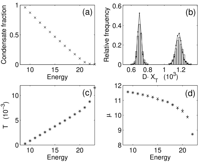
Figure 1: Data extracted from PGPE simulations in equilibrium. (a) Condensate fraction versus energy of simulation. (b) Histograms of the quantity $\mathbf{\mathcal{D}}\cdot\mathbf{X}_{T}$ on the RHS of Eq. (4) for the simulations with $E=10$ and $E=11$. The bars are for the operator $\mathbf{\mathcal{D}}_{Q}$, and the dots connected by solid lines for $\mathbf{\mathcal{D}}_{P}$. (c) Temperature versus energy. Plusses: $T_{Q}$, crosses: $T_{P}$. (d) Chemical potential versus energy. Plusses: $\mu_{Q}$, crosses: $\mu_{P}$. All quantities are in dimensionless units as defined in the text.

Figure 1(a) shows the condensate fraction versus energy for the PGPE system (we remind the reader that energy given by Eq. (12) is a conserved quantity in these calculations). The condensate fraction is determined by the Penrose-Onsager criterion: it is the largest eigenvalue found by diagonalizing the single-particle density matrix formed by ergodic averaging as described in Blakie2005a . It looks somewhat different to the result for the full three-dimensional system due to the basis cutoff that is present in these simulations. Figure 1(b) shows the distribution of the function $\mathbf{\mathcal{D}}\cdot\mathbf{X}_{T}$ for two different simulations, using the formulae for both $\mathbf{\mathcal{D}}_{Q}$ and $\mathbf{\mathcal{D}}_{P}$. The temperature is found by the inverse of the mean value of these distributions, and is shown for all simulations in Fig. 1(c). We can see that the results of both calculations agree very well, and so we can be confident that firstly the simulations have reached equilibrium, and secondly that the numerical implementation of these calculations are free from errors. Figure 1(d) shows the similar calculation for the chemical potential.

One interesting point is that the width of the distributions in Fig. 1(b) calculated using the operator $\mathbf{\mathcal{D}}_{P}$ are slightly narrower than those for $\mathbf{\mathcal{D}}_{Q}$. While this is of no consequence conceptually, in practice the narrower the distribution the fewer samples are required for an estimate of the mean to a required accuracy. Given the large amount of freedom in the choice of the operator $\mathbf{\mathcal{D}}$, it seems quite possible that for particular problems that some choices will be better than others. We have found situations where one of these distributions is signficantly narrower than the other. This has also been pointed out by Rugh Rugh2001a . However, with no a priori way to estimate the width of the distributions, finding the most accurate method of determing the temperature is a matter of trial and error.

V Conclusions

To investigate the effect of critical fluctuations in Bose gases using the PGPE in the microcanonical ensemble it is necessary to have accurate methods of determining the thermodynamic temperature and chemical potential. In this paper we have explicitly outlined a method of how to do so using the assumption of ergodicity and the dynamical evolution of the PGPE. The method could potentially be applied to other nonlinear classical field Hamiltonians.

References

• (1) Lee T D and Yang C N 1957 Phys. Rev. 105(3) 1119
• (2) Lee T D and Yang C N 1958 Phys. Rev. 112(5) 1419
• (3) Baym G, Blaizot J P, Holzmann M, Laloë F and Vautherin D 1999 Phys. Rev. Lett. 83(9) 1703
• (4) Arnold P and Moore G 2001 Phys. Rev. Lett. 87(12) 120401
• (5) Kashurnikov V A, Prokof’ev N V and Svistunov B V 2001 Phys. Rev. Lett. 87(12) 120402
• (6) Andersen J O 2004 Rev. Mod. Phys. 76 599
• (7) Holzmann M, Jean-Noël-Fuchs, Baym G A, Blaizot J P and Laloë F 2004 C. R. Physique 5 21
• (8) Svistunov B V and Shlyapnikov G V 1991 J. Mosc. Phys. Soc. 1 373
• (9) Kagan Y, Svistunov B V and Shlyapnikov G V 1992 Zh. Éksp. Teor. Fiz. 101 528 [JETP 75, 387 (1992)]
• (10) Kagan Y and Svistunov B V 1994 Zh. Éksp. Teor. Fiz. 105 353 [JETP 75, 387 (1992)]
• (11) Kagan Y and Svistunov B V 1997 Phys. Rev. Lett. 79 3331
• (12) Davis M J, Ballagh R J and Burnett K 2001 J. Phys. B 34 4487
• (13) Davis M J, Morgan S A and Burnett K 2001 Phys. Rev. Lett. 87 160402
• (14) Davis M J, Morgan S A and Burnett K 2002 Phys. Rev. A. 66 053618
• (15) Blakie P B and Davis M J 2005 http://arXiv.org pp cond–mat/0410496
• (16) Blakie P B and Davis M J 2005 http://arXiv.org pp cond–mat/0508669
• (17) Davis M J and Blakie P B 2005 http://arXiv.org pp cond–mat/0508667
• (18) Rugh H H 1997 Phys. Rev. Lett. 78 772
• (19) Davis M J and Morgan S A 2003 Phys. Rev. A 68(5) 053615
• (20) Gerbier F, Thywissen J H, Richard S, Hugbart M, Bouyer P and Aspect A 2004 Phys. Rev. Lett. 92(3) 030405
• (21) Rugh H H 2001 Phys. Rev. E 64 055101
• (22) Rugh H H 1998 J. Phys. A 31 7761
• (23) Giardina C and Livi R 1998 J. Stat. Phys. 91 1027
• (24) Jepps O G, Ayton G and Evans D J 2000 Phys. Rev. E 62 4757
• (25) Rickayzen G and Powles J G 2001 J. Chem. Phys. 114 4333