Critical temperature of a trapped Bose gas: comparison of theory and experiment

Abstract

We apply the Projected Gross-Pitaevskii equation (PGPE) formalism to the experimental problem of the shift in critical temperature $T_{c}$ of a harmonically confined Bose gas as reported in Gerbier et al. [Phys. Rev. Lett. 92, 030405 (2004)]. The PGPE method includes critical fluctuations and we find the results differ from various mean-field theories, and are in best agreement with experimental data. To unequivocally observe beyond mean-field effects, however, the experimental precision must either improve by an order of magnitude, or consider more strongly interacting systems. This is the first application of a classical field method to make quantitative comparison with experiment.

The shift in critical temperature $T_{c}$ with interaction strength for the homogeneous Bose gas has been the subject of numerous studies spanning almost fifty years since the first calculations of Lee and Yang Lee and Yang (1957, 1958). While there is a finite shift to the chemical potential in mean-field (MF) theory, the shift of the critical temperature is zero Baym et al. (2001). The leading order effect is due to long-wavelength critical fluctuations and is inherently non-perturbative. Using effective field theory it was determined that the shift is $\Delta T_{c}/T_{c}^{0}=can^{1/3}$ where $n$ is the particle number density, $a$ is the s-wave scattering length, and $c$ is a constant of order unity Baym et al. (1999). Until recently results for the value of $c$ disagreed by an order of magnitude and even sign, as summarised in Fig. 1 of Arnold and Moore (2001). However, two calculations performed using lattice Monte Carlo have settled the matter, and confirm that the shift is in the positive direction with combined estimate of $c\approx 1.31\pm 0.02$ Kashurnikov et al. (2001); Arnold and Moore (2001). A number of recent improved results broadly agree, and useful discussions are provided by Andersen Andersen (2004) and Holzmann et al. Holzmann et al. (2004).

The situation for the harmonically confined Bose gas is somewhat different. The ideal gas transition temperature and de Broglie wavelength at $T_{c}$ are

$$T_{c}^{0}=\left(\frac{N}{\zeta(3)}\right)^{1/3}\frac{\hbar\bar{\omega}}{k_{B}},\quad\lambda_{0}=\left(\frac{2\pi\hbar^{2}}{mk_{B}T_{c}^{0}}\right)^{1/2},$$ (1)

with $\bar{\omega}=(\omega_{x}\omega_{y}\omega_{z})^{1/3}$. There is a shift in $T_{c}$ due to finite size effects Grossmann and Holthaus (1995) given by $\Delta T_{c}/T_{c}^{0}\simeq-0.73N^{-1/3}\bar{\omega}/\omega$ with $\omega=(\omega_{x}+\omega_{y}+\omega_{z})/3$, however this is usually small for experimentally relevant parameters. The first-order shift in $T_{c}$ that survives in the thermodynamic limit is due to mean-field effects and has been estimated analytically Giorgini et al. (1996). Repulsive interactions reduce $T_{c}$, which can be intuitively understood due to a lowering of the peak density of the gas. Next-order effects due to fluctuations have been estimated in Houbiers et al. (1997); Arnold and Tomášik (2001); Holzmann et al. (2004) and in general predict an increase in $T_{c}$ from the first order result. For a sufficiently wide trap Ref. Arnold and Tomášik (2001) estimates

$$\frac{\Delta T_{c}}{T_{c}^{0}}=c_{1}\frac{a}{\lambda_{0}}+\left(c_{2}^{\prime}\ln\frac{a}{\lambda_{0}}+c_{2}^{\prime\prime}\right)\left(\frac{a}{\lambda_{0}}\right)^{2}+O\left(\frac{a}{\lambda_{0}}\right)^{3},$$ (2)

with $c_{1}=-3.426$, $c_{2}^{\prime}=-45.86$, $c_{2}^{\prime\prime}=-155.0$, which for $a/\lambda_{0}<0.032$ predicts a positive shift due to fluctuations. The first term is the MF result of Giorgini et al. (1996). Recently Zobay and co-authors have investigated power law traps with the goal of understanding how $T_{c}$ behaves in a smooth transition from harmonic trapping to the homogeneous situation Zobay (2004); Zobay et al. (2004, 2005).

For a typical BEC experiment, the critical temperature deviates from the ideal gas result only by a few percent. As thermometry of Bose gases at this level of accuracy can be difficult Gerbier et al. (2004a), until recently the only experimental measurement was reported by Ensher et al.  with $\Delta T_{c}/T_{c}^{0}=-0.06\pm 0.05$ Ensher et al. (1996). However, in 2004 the Orsay group reported precise measurements of the critical temperature for a range of atom numbers, and compared their results to the first-order MF estimate of Giorgini et al. (1996). While in agreement, the theoretical results lie near the upper range of the experimental error bars.

Previously one of us used the classical field projected Gross-Pitaevskii equation (PGPE) formalism Davis et al. (2001a, b, 2002) to give an estimate of the shift in $T_{c}$ of the homogeneous Bose gas Davis and Morgan (2003), which was found to be in agreement with the Monte Carlo calculations Kashurnikov et al. (2001); Arnold and Moore (2001). The PGPE is a dynamical non-perturbative method, with the only approximation being that the highly occupied modes ($\langle N_{k}\rangle\gg 1$) of the quantum Bose field are well-approximated by a classical field evolved according to the GPE. Related classical field approaches have been considered by a number of authors, including Kagan and co-workers Kagan and Svistunov (1997), Sinatra et al. Sinatra et al. (2000, 2001), Rza̧żewski and co-workers Góral et al. (2001, 2002).

Here we use an extension of the PGPE for harmonically trapped gases Blakie and Davis (2005) to calculate the shift in $T_{c}$ for the experiment of Gerbier et al., and in particular focus on the competing effects of mean-field and critical fluctuations. The PGPE in dimensionless units is

$$i\frac{\partial\Psi}{\partial\tau} = -\nabla^{2}\Psi+V\Psi+\mathcal{P}\{C_{\rm nl}|\Psi|^{2}\Psi\},$$ (3)

where $\Psi$ is the classical field, $V=(\lambda_{x}^{2}x^{2}+\lambda_{y}^{2}y^{2}+z^{2})/4$, and $\lambda_{x,y}=\omega_{x,y}/\omega_{z}$. The nonlinearity is $C_{\rm nl}=N_{b}U_{0}/\hbar\omega_{z}x_{0}^{3}$ where the unit of length is $x_{0}=\sqrt{\hbar/2m\omega_{z}}$ and $\tau=\omega_{z}t$. For the harmonic trap the Bose field is expanded on a basis of harmonic oscillator eigenstates, with the cutoff energy $E_{\mathrm{cut}}$ determined by the occupation number condition. The projection operator $\mathcal{P}\{F\}$ projects the function $F$ onto the harmonic oscillator modes with energy less than $E_{\mathrm{cut}}$.

The dynamical PGPE system represents a microcanonical ensemble, and will evolve any random initial conditions to thermal equilibrium defined by the integrals of motion Davis et al. (2001b). For a cylindrically symmetric harmonic trap these are the total number of particles, the energy, and the component of the angular momentum along the symmetry axis. Once in equilibrium, we use the assumption of ergodicity to accurately determine the condensate fraction Blakie and Davis (2005), and the temperature $T$ and chemical potential $\mu_{b}$ Davis and Morgan (2003). By varying the initial state energy we measure the dependence of condensate fraction on temperature.

As an initial investigation into critical fluctuations, in Fig. 1 the results of the PGPE calculations from Blakie and Davis (2005) are compared with a self-consistent mean-field calculation in the Popov approximation to the Hartree-Fock-Bogoliubov (HFB) formalism (see e.g. Hutchinson et al. (1997)). In order to make a direct comparison, the HFB-Popov calculation is performed in the same basis as the dynamical PGPE calculations, and we use the equipartition distribution $N_{k}=k_{B}T/(\epsilon_{k}-\mu)$ for the quasi-particle occupations. (This is the high temperature limit $k_{B}T\gg\epsilon_{k}$ of the Bose-Einstein distribution applicable to classical fields). For smaller values of $C_{\mathrm{nl}}$ the HFB-Popov theory agrees with the classical field calculation, however for larger values there is a distinct difference which we attribute to critical fluctuations. We have repeated these calculations using gapless implementations of HFB theory Proukakis et al. (1998) and found that they are little different from the results calculated using HFB-Popov. Our results demonstrate that critical fluctuations have a measurable effect for the PGPE system. However this is an idealised calculation — to be quantitative we must make a connection between the PGPE method and the recent experiment Gerbier et al. (2004b).

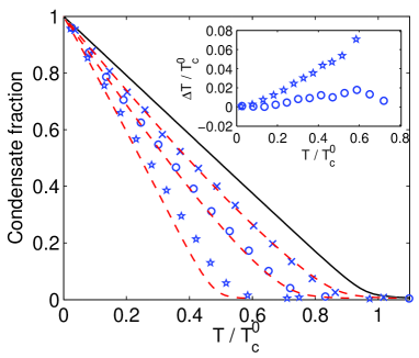
Figure 1: (color online) Comparison of condensate fraction versus temperature normalised to $T_{c}^{0}$ for the PGPE method and the HFB-Popov calculation for $\lambda_{x}=\sqrt{8},\,\lambda_{y}=1$ and $E_{{\rm cut}}=31\hbar\omega_{z}$. PGPE method: $C_{\mathrm{nl}}=500$ (crosses), $C_{\mathrm{nl}}=2000$ (circles), $C_{\mathrm{nl}}=10000$ (stars). Dashed line: HFB-Popov results. Solid line: exact result for $C_{\mathrm{nl}}=0$. Inset: $\Delta T=T_{\rm PGPE}-T_{\rm HFB}$ at fixed condensate fraction for $C_{\mathrm{nl}}=2000$ and $10000$, indicating a maximum shift near $T_{c}$.

$N_{\rm tot}^{0}$ ($10^{6}$)	0.5	1.0	1.5	2.0	2.5	2.5	3.0	4.0	5.0
$T_{c}^{0}$ (nK)	399	505	580	639	689	689	733	808	871
$N_{\rm cut}$	5.0	5.0	5.0	5.0	5.0	7.5	7.5	7.5	7.5
$E_{\rm cut}$ ($\hbar\omega_{z}$)	219	266	299	325	347	253	266	288	307
Modes	767	1382	1952	2498	3058	1172	1373	1730	2129
$N_{\rm b}(10^{3})$	8.75	15.0	20.7	26.1	31.4	19.2	22.1	27.6	33.1
$\mu_{c}$ ($\hbar\omega_{z}$)	101	119	132	142	152	135	143	153	163
$\delta_{c}$ ($\hbar\omega_{z}$)	23	29	34	37	41	39	41	46	49

Table 1: Input parameters for the PGPE simulations. The chemical potential $\mu_{b}$ and the shift of the cutoff energy $\delta_{c}$ are outputs parameters measured at the critical point.

Gerbier et al. Gerbier et al. (2004b) trap ⁸⁷Rb atoms in a cylindrically symmetric harmonic potential with $(\omega_{x,y},\omega_{z})=2\pi\times(413,8.69)$ Hz giving $\lambda_{x,y}=47.52$. For total numbers of atoms $N_{\mathrm{tot}}$ ranging from $2.5\times 10^{5}$ to $2.5\times 10^{6}$, the critical point was identified by reducing the final rf frequency of the evaporative cooling, and identifying the point that the condensate fraction became measurable (see Fig. 2 of Gerbier et al. (2004b).) We perform numerical simulations in a similar manner. We choose relevant simulation parameters and dynamically evolve the system to equilibrium for a range of energies. We identify the critical point from the number of condensate particles and determine the number of particles above the cutoff using a self-consistent semi-classical approximation for the high-energy modes as described below. This gives us a set of points $(N_{c},T_{c})$ to be compared with the experimental data.

To simulate the experiments of Gerbier et al. using the PGPE we need to choose both an energy cutoff $E_{\rm cut}$ and a number of particles below the cutoff $N_{b}$ to simulate so that the occupation number condition is satisfied. However, any final result should be insensitive to the exact value of the cutoff that is chosen. A priori estimates for our simulation parameters were determined from the Bose-Einstein distribution of quantum orbitals of an ideal trapped gas at the critical temperature, and are summarised in Table 1. For the smaller clouds we chose an energy cutoff such that $\langle N_{k}\rangle\geq 5$. For the large clouds this leads to correspondingly larger basis sets that become computationally prohibitive, and for these we chose $\langle N_{k}\rangle\geq 7.5$. In principle we could use this occupation condition for all simulations, however the two calculations at the crossover point ($N_{\rm{tot}}^{0}=2.5\times 10^{6}$) enables us to verify that our calculations are insensitive to the exact value of the energy cutoff. We use the PGPE to evolve randomised initial states to equilibrium and measure the condensate number $N_{0}$, chemical potential $\mu_{b}$, temperature $T$, and density $n_{b}(\mathbf{x})$ for each set of parameters.

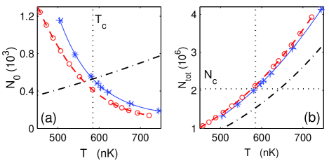
Figure 2: (color online) Determination of the critical number and temperature for the simulation with $N_{\mathrm{tot}}^{0}=4.0\times 10^{6}$. (a) $N_{0}$ vs $T$ for: classical field (crosses, plusses, solid line), HFB-Popov (circles, dashed line). The number of condensate atoms for the ideal gas at the critical temperature is the dot-dash line. (b) Total number of atoms for: classical field (crosses, plusses, solid line), HFB-Popov (circles, dashed line). Critical number versus temperature for the finite-sized ideal gas is the dot-dash line. For both (a) and (b) the solid and dashed lines are polynomial fits to the data.

In Fig. 2(a) we plot the condensate number versus temperature for the $N_{\rm tot}^{0}=4\times 10^{6}$ data set and find there is no sharp transition. This is because we are only considering the atoms below the cutoff. As the majority of atoms in the full system are above the cutoff and $N_{0}$ is of order a few hundred particles for all the data points on this graph, these simulation results all lie close to the critical point. To determine a single critical point from each data set we plot on the same graph the corresponding condensate number for the finite-sized ideal gas at the same critical temperature. We choose the intersection of these two curves to identify the critical point, and have verified that the occupation number condition is satisfied here.

To relate these results back to the full experimental system we assume that the classical field and the above cutoff thermal cloud are weakly-coupled systems in equilibrium, with the same temperature and chemical potential. The thermal cloud exists in the potential of the trap plus time-averaged classical field density $n_{b}(\mathbf{x})$ that is determined from the PGPE simulations. To solve for the above cutoff thermal cloud we make use of the self-consistent Hartree-Fock approximation, which provides an accurate description of the modes above $E_{\mathrm{cut}}$. The above cutoff density is determined by the self-consistent solution of

$$n_{a}(\mathbf{x})=\frac{1}{h^{3}}\int_{E_{\mathrm{HF}}>E_{0}}d^{3}\mathbf{p}\left[e^{(E_{\mathrm{HF}}(\mathbf{p},\mathbf{x})-\mu)/k_{B}T}-1\right]^{-1},$$ (4)

$$E_{\mathrm{HF}}(\mathbf{p},\mathbf{x})=p^{2}/2m+V_{\rm trap}(\mathbf{x})+2U_{0}[n_{b}(\mathbf{x})+n_{a}(\mathbf{x})],$$ (5)

where $E_{\mathrm{HF}}(\mathbf{p},\mathbf{x})$ is the Hartree-Fock energy. In this procedure the contribution of the above cutoff density $n_{a}(\mathbf{x})$ to the effective potential for the classical field is neglected. This is justified as we find that near the critical point $n_{a}(\mathbf{x})$ is approximately flat in the region where the $n_{b}(\mathbf{x})$ is non-zero. However, the uniform energy shift of this interaction must be included in the chemical potential used in Eq. (4) as $\mu=\mu_{b}+2n_{a}(\mathbf{0})U_{0}$. Another important correction accounts for the shift in the energy of the highest oscillator modes in the classical field from $E_{\mathrm{cut}}$ due to interaction effects so that the integral in Eq. (4) is over the correct region of phase space. We do this by assuming that the highest energy modes of the classical field are single-particle in nature, and are shifted by a constant amount $\delta_{c}$. We fit the time-averaged occupation of these modes to $\langle N_{k}\rangle=T/(\epsilon_{k}^{0}+\delta_{c}-\mu_{b})$. The lower limit of the integral in Eq. (4) is then $E_{0}=E_{\mathrm{cut}}+\delta_{c}+2n_{a}(\mathbf{0})U_{0}$ to account for the mean-field of the thermal cloud.

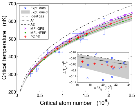
Figure 3: (color online) Comparison of theoretical calculations with experiment. The main figure plots $T_{c}$ vs $N_{c}$, whereas the inset plots the shift of $T_{c}$ against the relevant small parameter $a/\lambda_{0}$. Experimental results: data (open circles), one $\sigma$ fit (grey area). Theoretical results for $T_{c}$: ideal gas (dot-dash), A1 (dotted), A2 (dashed), MF-GPE (crosses), MF-HFBP (dots), PGPE (plusses). Solid lines through the data points are polynomial fits. A1 is not shown in the main figure for clarity.

We have also calculated $T_{c}$ using other methods for comparison, as summarised below:
1. A1: This is the first order analytic estimate of Giorgini et al. Giorgini et al. (1996), which is the first term of Eq. (2).
2. A2: This is the full second order result of Eq. (2). However, the validity condition for this result (Eq. (7.2) of Arnold and Tomášik (2001)) requires the trap to be “sufficiently broad”, and this is strongly violated for this experiment. This essentially says that the semi-classical approximation is not valid for the lowest energy modes of this strongly elongated system.
3. MF-GPE: The GPE is solved numerically using a variational Gaussian ansatz, and the thermal cloud calculated using a semi-classical approximation Giorgini et al. (1996). At each temperature the condensate and non-condensate are determined self-consistently with a fixed number of particles, and the critical temperature is where the condensate fraction decreases to zero.
4. MF-HFBP: We fix the condensate fraction, and determine the temperature that gives an appropriate self-consistent condensate mode and thermal density. We have verified the results are unchanged for equipartition or Bose-Einstein statistics. We use the same procedure as for the PGPE calculation to determine the critical point, the above cutoff density and the total atom number. An illustrative set of data is displayed in Fig. 2.

In Fig. 3 we compare these theoretical results with the PGPE and experimental data. The MF A1 estimate was shown in Gerbier et al. (2004b) and is within the experimental error bars. However, our more accurate MF-GPE calculation gives a greater value of $T_{c}$ at larger atom numbers, agreeing with the mean-field results of Houbiers et al. Houbiers et al. (1997). However, the MF-HFBP result, which presumably is an even better mean-field calculation, is quite different and towards the lower end of the experimental error estimate.

The predicted effect of critical fluctuations Houbiers et al. (1997); Arnold and Tomášik (2001) is to further increase $T_{c}$. The non-perturbative A2 estimate lies at the boundary of experimental error, but as mentioned earlier this result does not satisfy the validity requirement for this experiment. The PGPE calculation, which includes all the physics of the MF-HFBP calculation as well as critical fluctuations, is measurably different. Arguably it is in best agreement with the experimental data. However, both the PGPE and MF-HFBP calculations lie within the error bars, suggesting that experimental precision must improve by an order of magnitude in order to distinguish these predictions.

The inset of Fig. 3 shows the PGPE shift as a function of $a/\lambda_{0}$ and in comparison with the results of Eq. (2) and the experimental data. The second order term is almost constant over the experimental range of $a/\lambda_{0}$ and so cannot distinguish the presence or otherwise of any logarithmic term. We note that the finite-size shift is subtracted from the PGPE and experimental data for this comparison.

We have also translated data for parameters as in Fig. 1 but with $C_{\mathrm{nl}}=5000$ to realistic experimental values, and found that for $10^{7}$ atoms of ⁸⁷Rb in a TOP trap with a 40 Hz radial frequency that the difference between the MF-HFBP and PGPE results is of order 3%. Thus we suggest that for currently accessible experimental conditions it will be necessary to either make use of Feshbach resonances to probe more strongly interacting regimes, or to move to traps flatter than harmonic to be able to distinguish these theories in the lab.

In conclusion we have performed a careful theoretical analysis of the experiment on the shift in critical temperature of a trapped Bose gas reported in Gerbier et al. Gerbier et al. (2004b). We have determined that earlier calculations based on mean-field theory and the local-density approximation are inappropriate for this experiment, and make predications for $T_{c}$ outside the experimental error bars at larger atom numbers. We have applied non-perturbative classical field theory to this problem, and described how to incorporate the physics of the above-cutoff atoms in equilibrium. The results include the effect of critical fluctuations, and give the best agreement with experimental observations. Our results indicate the precision requirements for experiments to investigate beyond mean-field effects on the critical temperature.

We thank Alain Aspect for useful discussions. MJD acknowledges financial support from the Australian Research Council and the University of Queensland, and PBB from the Marsden Fund of New Zealand and the University of Otago.

References

- Lee and Yang (1957) T. D. Lee and C. N. Yang, Phys. Rev. 105, 1119 (1957).
- Lee and Yang (1958) T. D. Lee and C. N. Yang, Phys. Rev. 112, 1419 (1958).
- Baym et al. (2001) G. Baym, J.-P. Blaizot, M. Holzmann, F. Laloë, and D. Vautherin, Eur. Phys. J. B 24, 107 (2001).
- Baym et al. (1999) G. Baym, J.-P. Blaizot, M. Holzmann, F. Laloë, and D. Vautherin, Phys. Rev. Lett. 83, 1703 (1999).
- Arnold and Moore (2001) P. Arnold and G. Moore, Phys. Rev. Lett. 87, 120401 (2001).
- Kashurnikov et al. (2001) V. A. Kashurnikov, N. V. Prokof’ev, and B. V. Svistunov, Phys. Rev. Lett. 87, 120402 (2001).
- Andersen (2004) J. O. Andersen, Rev. Mod. Phys. 76, 599 (2004).
- Holzmann et al. (2004) M. Holzmann, J.-N. Fuchs, G. A. Baym, J.-P. Blaizot, and F. Laloë, C. R. Physique 5, 21 (2004).
- Grossmann and Holthaus (1995) S. Grossmann and M. Holthaus, Phys. Lett. A 208, 188 (1995).
- Giorgini et al. (1996) S. Giorgini, L. P. Pitaevskii, and S. Stringari, Phys. Rev. A 54, R4633 (1996).
- Houbiers et al. (1997) M. Houbiers, H. T. C. Stoof, and E. A. Cornell, Phys. Rev. A 56, 2041 (1997).
- Arnold and Tomášik (2001) P. Arnold and B. Tomášik, Phys. Rev. A 64, 053609 (2001).
- Zobay (2004) O. Zobay, J. Phys. B 37, 2593 (2004).
- Zobay et al. (2004) O. Zobay, G. Metikas, and G. Alber, Phys. Rev. A 69, 063615 (2004).
- Zobay et al. (2005) O. Zobay, G. Metikas, and H. Kleinert, Phys. Rev. A 71, 043614 (2005).
- Gerbier et al. (2004a) F. Gerbier, J. H. Thywissen, S. Richard, M. Hugbart, P. Bouyer, and A. Aspect, Phys. Rev. A 70, 013607 (2004a).
- Ensher et al. (1996) J. R. Ensher, D. S. Jin, M. R. Matthews, C. E. Wieman, and E. A. Cornell, Phys. Rev. Lett. 77, 4984 (1996).
- Davis et al. (2001a) M. J. Davis, R. J. Ballagh, and K. Burnett, J. Phys. B 34, 4487 (2001a).
- Davis et al. (2001b) M. J. Davis, S. A. Morgan, and K. Burnett, Phys. Rev. Lett. 87, 160402 (2001b).
- Davis et al. (2002) M. J. Davis, S. A. Morgan, and K. Burnett, Phys. Rev. A. 66, 053618 (2002).
- Davis and Morgan (2003) M. J. Davis and S. A. Morgan, Phys. Rev. A 68, 053615 (2003).
- Kagan and Svistunov (1997) Y. Kagan and B. V. Svistunov, Phys. Rev. Lett. 79, 3331 (1997).
- Sinatra et al. (2000) A. Sinatra, Y. Castin, and C. Lobo, J. Mod. Opt. 47, 2629 (2000).
- Sinatra et al. (2001) A. Sinatra, C. Lobo, and Y. Castin, Phys. Rev. Lett. 87, 210404 (2001).
- Góral et al. (2001) K. Góral, B.-G. Englert, and K. Rza̧żewski, Phys. Rev. A 63, 033606 (2001).
- Góral et al. (2002) K. Góral, M. Gajda, and K. Rza̧żewski, Phys. Rev. A 66, 051602(R) (2002).
- Blakie and Davis (2005) P. B. Blakie and M. J. Davis, Phys. Rev. A 72, 063608 (2005).
- Hutchinson et al. (1997) D. A. W. Hutchinson, E. Zaremba, and A. Griffin, Phys. Rev. Lett. 78, 1842 (1997).
- Proukakis et al. (1998) N. P. Proukakis, S. A. Morgan, S. Choi, and K. Burnett, Phys. Rev. A 58, 2435 (1998).
- Gerbier et al. (2004b) F. Gerbier, J. H. Thywissen, S. Richard, M. Hugbart, P. Bouyer, and A. Aspect, Phys. Rev. Lett. 92, 030405 (2004b).