Ordering of geometrically frustrated classical and quantum Ising magnets

Abstract

A systematic study of both classical and quantum geometric frustrated Ising models with a competing ordering mechanism is reported in this paper. The ordering comes in the classical case from a coupling of 2D layers and in the quantum model from the quantum dynamics induced by a transverse field. By mapping the Ising models on a triangular lattice to elastic lattices of non-crossing strings, we derive an exact relation between the spin variables and the displacement field of the strings. Using this map both for the classical (2+1)D stacked model and the quantum frustrated 2D system, we obtain a microscopic derivation of an effective Hamiltonian which was proposed before on phenomenological grounds within a Landau-Ginzburg-Wilson approach. In contrast to the latter approach, our derivation provides the coupling constants and hence the entire transverse field–versus–temperature phase diagram can be deduced, including the universality classes of both the quantum and the finite–temperature transitions. The structure of the ordered phase is obtained from a detailed entropy argument. We compare our predictions to recent simulations of the quantum system and find good agreement. We also analyze the connections to a dimer model on the hexagonal lattice and its height profile representation, providing a simple derivation of the continuum free energy and a physical explanation for the universality of the stiffness of the height profile for anisotropic couplings.

I Introduction

Frustrated two-dimensional magnetic systems exhibit a rich variety of phases and critical points. The consequences of quantum or thermal fluctuations about the highly degenerate ground states of frustrated magnets are important to understand in the ongoing quest to find novel exotic quantum states Sachdev-book . The past decades have seen a resurgence of significant interest in a systematic study of geometrically frustrated antiferromagnets Diep-book . Geometric frustration arises in materials containing antiferromagnetically coupled moments which reside on geometrical units, that inhibit the formation of a collinear magnetically ordered Néel state, and induces a macroscopically large degeneracy of the classical ground state.

For magnets with a discrete Ising symmetry, the complexity of the ground-state manifold can endow the system with a continuous symmetry. Such symmetry is of particular importance to 2D quantum magnets at low temperatures since then the Mermin-Wagner theorem applies, precluding an ordered phase Mermin+66 . Another possible but contrary scenario is “order-from-disorder” Villain+80 where zero-point fluctuations select a small class of states from the ground-state manifold since those states are particularly susceptible to fluctuations. This fundamental mechanism can produce an ordered symmetry-broken state moessner1 . Hence one expects weak competing fluctuations about the classical ground states to be able to generate new strongly correlated states and (quantum) phase transitions of unexpected universality classes.

From a theoretical perspective, it is natural to try to understand the role of frustration from extremely simple interactions and dynamics. The possibly simplest realization of classical frustration is found in the antiferromagnetic Ising model on a triangular lattice (TIAF). Each elementary triangle is frustrated, and the TIAF is disordered even at zero temperature with a finite entropy density and algebraic decaying spin correlations Wannier+Houtappel . The effect of quantum fluctuations about the highly degenerate ground states can be studied in its simplest form by introducing quantum spin dynamics from a magnetic field which is transverse to the spin coupling. For this transverse field TIAF model, and its companions on other 2D lattices, Moessner and Sondhi have argued the existence of both ordered and spin liquid phases moessner1 . In the limit of a small field, the quantum ground state is constructed as a linear superposition of classical ground states which maximize the number of spins which can be flipped to gain transversal field energy at no cost in exchange energy. This yields a strong suppression of configurations and, since the TIAF is already critical at zero field, order emerges. As a result, there will be a discontinuity in entropy and correlations in the ground state at vanishing field and zero temperature. At a large transverse field, the TIAF has a gaped paramagnetic ground state. It is separated from the ordered state by a quantum critical point. The additional effect of thermal fluctuations has been studied quantitatively so far only in simulations Isakov+03 .

Experimental realizations of these frustrated Ising systems can be found either directly in magnets with strong anisotropy, e.g., in LiHoF₄ Aeppli+98 , or indirectly (via the equivalent (2+1)D classical model) in stacked triangular lattice antiferromagnets Collins+97 with strong couplings along the stacking direction as studied in recent experiments on CsCoBr₃ Mao+02 . However, transverse field Ising models can also provide insight into some more complicated systems in certain limits. They may describe the singlet sector below the spin gap of frustrated antiferromagnetic quantum Heisenberg models, e.g., on the Kagome lattice, since the latter model can then be formulated as a ${\mathbb{Z}}_{2}$ gauge theory which in turn is related by duality to the transverse field Ising system on the dual lattice of the original Heisenberg model Nikolic+03 . An ordered Ising phase describes then in the Heisenberg problem a paramagnet with spin waves forming the gaped excitations. A related approach to study Heisenberg antiferromagnets is via quantum dimer models (QDM) on the same lattice Rokhsar+98 . Depending on the lattice symmetry, the QDM exhibits a disordered state (on the triangular lattice) Moessner+01a ; Moessner+01b , corresponding to a resonating valence bond or spin-liquid phase, or it is found always in ordered valence-bond solid phases (on the hexagonal lattice) Moessner+01a ; Moessner+01b . Interestingly, the spin liquid phase renders the triangular QDM a promising candidate for quantum computing Ioffe+02 . For Ising spins, there is also a direct correspondence between QDM’s with just kinetic terms and fully frustrated Ising models in a small transverse field on the dual lattice moessner1 . In particular, the transverse field TIAF maps to the hexagonal QDM.

For comparison to the new developments presented in this work, we briefly review the salient achievements for the classical stacked and quantum TIAF obtained in earlier studies. Symmetry arguments have been used to guess a Landau-Ginzburg-Wilson (LGW) theory for the (2+1)D classical stacked system Blankschtein+84 . After translation to the quantum TIAF, this approach suggests a quantum critical point of 3D XY universality at intermediate transverse field strength and an extended critical phase at finite temperatures moessner1 . However, the Suzuki-Trotter mapping relating the 2D quantum and (2+1)D classical systems involves a scaling limit with a diverging anisotropy of the classical exchange coupling which may invalidate a LGW approach suzuki1 . Moreover, the latter approach has been put somewhat into question, mainly since it has been argued that it fails to describe the (classical) system at low temperatures since it neglects the restriction to classical spin values $\pm 1$ and thus geometrical frustration Coppersmith85 . Very recent Monte Carlo simulation support the LGW based conjecture for the phase diagram but the actual computations were performed for the (2+1)D classical problem Isakov+03 . Recently, the weak field behavior has been also studied in terms of a quantum kink crystal Mostovoy+03 .

In a recent letter Jiang+05 the present authors have presented a string description of the transverse field TIAF in order to obtain a quantitative prediction for the phase diagram. In the present paper, we will give a full account of the relation between spins and non-crossing strings, including a more complete presentation of the relation to dimer models and its surface height representation. We exploit and extend the quantum dimer analogy in order to map the TIAF, at arbitrary transverse field strength, to quantum strings which result from the superposition of dimer configurations plus defects and a fixed reference dimer state. Using the Suzuki-Trotter theorem suzuki1 we obtain a stack of coupled 2D layers of classical strings which in the Suzuki-Trotter limit of infinitely many layers can be described by the Villain model Villain75 . We show that the LGW action Blankschtein+84 , which was employed in the vicinity of the quantum critical point moessner1 , can be derived microscopically from the quantum string action if the phase of the complex LGW order parameter is identified with the displacement field of the string lattice. However, our approach explicitly takes into account frustration which is encoded in the topological constraint on the phase field resulting from the non-crossing property of the strings. This constraint restricts the phase field configurations of the order parameter and thus distinguishes our theory from the original LGW approach. Our approach confirms explicitly the 3D XY universality of the quantum critical point, and allows to predict the phase diagram at arbitrary transverse field strength and finite temperature. Using an entropy argument for the strings, we can determine the nature of the ordered phase.

In this paper we present first a thorough discussion of the relations between Ising spins on the triangular lattice, dimers on the hexagonal lattice and its height representation and elastic string lattices. After a introduction of the spin models in Section II, we explore the relations to dimers and strings in Section III for the classical 2D Ising model on the triangular lattice in order to set up the formalism for the following sections. In Section IV we map the Ising model on a stacked triangular lattice to (2+1)D string lattice which is described by a 3D XY model with a 6-fold symmetry breaking term. Using the results of the latter section, we perform a Suzuki-Trotter mapping of the 2D quantum Ising system to the classical stacked model which enables us to predict a quantitative phase diagram for the quantum frustrated model in Section V. Finally, we conclude with a summary and a discussion of potential extensions of our work in Section VI.

II Models

We are interested in two models which are both based on the Ising antiferromagnet on a triangular lattice (TIAF). First, we study a classical three dimensional Ising system which consists of a stack of TIAF’s which are coupled ferromagnetically. The Hamiltonian reads

$$H_{\rm 3D}=J_{\parallel}\sum_{\langle ij\rangle,k}\sigma_{ik}\sigma_{jk}-J_{\perp}\sum_{i,k}\sigma_{ik}\sigma_{ik+1},$$ (1)

with $\sigma_{ik}=\pm 1$ and where $J_{\parallel}$, $J_{\perp}>0$ and $\langle ij\rangle$ indicates summation over nearest-neighbor pairs in each TIAF plane. This system is fully frustrated in each layer, but has no competing interaction along the stacking direction. This model has been studied originally within a Landau-Ginzburg-Wilson (LGW) approach by Blankschtein et al. Blankschtein+84 . In fact, much of the physics of the stacked triangular lattice is similar to that of the two-dimensional triangular lattice. However, the presence of the third dimension has the tendency to stabilizes ordered phases. Indeed, for all well-characterized materials which have triangular magnetic lattices, the long-range order at low temperatures is three-dimensional in nature. The stacked system is of direct experimental relevance since it describes the low-temperature physics of the Ising-like compounds CsCoCl₃, CsCoBr₃ and related materials where transition metal atoms form chains along the stacking direction which are coupled through three equivalent halogen atoms. For a review on these compounds see Ref. Collins+97, . Almost the entire existing body of theory on this stacked system is based on the LGW approach, mean-field theory and numerical simulations with sometimes conflicting results for the low-temperature ordered phase. We will briefly review previous developments for this model in Section IV.

As shall be demonstrated below, the previously introduced model is also useful in describing the two-dimensional quantum antiferromagnet which results from applying a transverse magnetic field to the TIAF. The latter system has the Hamiltonian

$$H=J\sum_{\langle i,j\rangle}\,\sigma^{z}_{i}\sigma^{z}_{j}+\Gamma\sum_{i}\sigma^{x}_{i}\,,$$ (2)

$\sigma^{x}$, $\sigma^{z}$ are Pauli operators, and $\Gamma$ is the transverse field. This model is of particular interest since it combines a standard realization of geometric frustration with simple quantum dynamics. The transverse field induces tunnelling between the exponentially large number of classical ground states at zero temperature. One can argue that the quantum fluctuations select a smaller susceptible class of the ground states. This would lead then to a reduction of ground state entropy, and an “order from disorder” Villain+80 phenomenon is expected.

Both the classical stacked magnet and the 2D quantum TIAF are related to the quantum dimer model (QDM) on the hexagonal lattice.

III String picture of classical frustrated 2D magnets

III.1 From spins to dimers

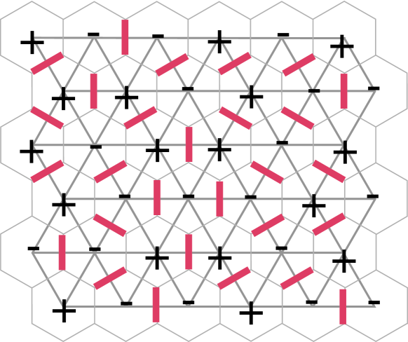
Figure 1: (color online) Mapping of a spin configuration to a dimer covering on the dual hexagonal lattice.

We start with the description of the antiferromagnetic Ising model on the triangular lattice in order to explain its relation to dimers and strings. The Hamiltonian is

$$H_{\rm TIAF}=\sum_{\langle i,j\rangle}J_{ij}\sigma_{i}\sigma_{j}$$ (3)

where the couplings $J_{ij}$ are equal to one of the three positive constants $J_{1}$, $J_{2}$ or $J_{3}$ depending on the orientation of the bond $(ij)$ relative to the three main lattice directions. It is well knownWannier+Houtappel that the ground state of this system has exponentially large degeneracy in the isotropic case $J_{1}=J_{2}=J_{3}$, leading to a finite entropy density and the absence of order even at zero temperature. For all ground states of the general model of Eq. (3) each triangle has exactly one frustrated bond, and hence there is a one-to-one correspondence (modulo a global spin flip) of all spin ground state configurations to complete dimer coverings of the dual hexagonal lattice. This can be seen from Fig. 1: If one places a dimer across every frustrated bond, one obtains the corresponding dimer covering of the dual hexagonal lattice, where each lattice site in the hexagonal lattice is touched by one and only one dimer Nienhuis+84 . If the two smallest couplings are equal, $J_{1}=J_{3}<J_{2}$, then dimers can occupy bonds in directions $1$ and $3$ only and there is still a huge ground state degeneracy. But the entropy at $T=0$ scales now $\sim\sqrt{N}$ with the number of lattice sites, $N$, due to the constraint that dimers cannot touch each other. Thus the entropy density vanishes and the system is ordered at $T=0$ but disordered at any finite temperature. (At finite $T$ topological defects have to be considered, see below.) If one of the three coupling constants is the smallest, then there is only one dimer ground state configuration with all dimers being perpendicular to the direction with smallest coupling, and order survives at finite temperature.

The analogy to dimers can be expressed by the fact that the Ising partition function in the limit of vanishing temperature is proportional to that of the dimers which reads

$$Z_{D}=\sum_{\{D\}}z_{1}^{n_{1}}z_{2}^{n_{2}}\,,$$ (4)

where the sum runs over all complete dimer coverings of the hexagonal lattice, and $n_{1}$ and $n_{2}$ is the number of dimers being perpendicular to direction 1 and 2, respectively. Here we assumed that $J_{3}\leq J_{1}$, $J_{2}$ so that the weights for the two types of non-vertical bonds are given by

$$z_{1}=e^{-2(J_{1}-J_{3})/T},\;z_{2}=e^{-2(J_{2}-J_{3})/T},$$ (5)

and all vertical bonds have a weight of unity. Of course, for the TIAF the isotropic case with $J_{1}=J_{2}=J_{3}$ is of most interest but for the dimer model itself anisotropic weights provide some interesting insight as will become clear below. We note that even at finite temperature the analogy to dimers will turn out to be useful but then defects (triangles with all three bonds crossed by dimers) have to be included.

III.2 From dimers to strings

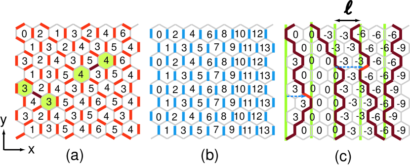
Figure 2: (color online) Mapping a dimer covering (a) to a string configuration (c) via the reference state (b). The numbers denote the height profiles associated with the dimer coverings. The displacement of a string from its straight reference position is determined by the height profile at the two plaquettes which are joined by the displaced dimer in the original dimer covering (a).

In this subsection we make use of another mapping which relates dimer configurations to fluctuating strings which are directed and non-crossing yokoi+86 . This mapping applies to general weights for the dimers but of primary interest is the TIAF at $T=0$ where the dimer weights are either unity or zero, and there is a one-to-one correspondence (modulo a global spin flip) of Ising ground states to string configurations. The string representation results from the superposition of a given dimer covering and a fixed reference dimer covering where all vertical bonds of the hexagonal lattice are occupied by dimers, see Fig. 2(b). The superposition is an ”exclusive or” operation, i.e., only if a given bond is covered by a dimer either in the original covering or in the reference covering, it will be covered in the superposition. The resulting superposition is no longer a dimer covering (since dimers touch each other) but an array of strings which are directed (along the reference direction) and non-crossing (due to the fact that each site is touched by exactly one dimer in the original dimer covering) zeng1 . The fluctuations of the lines result from the non-zero entropy density of the spin system. Or in other words, we map the zero temperature TIAF to a line lattice at a finite (virtual) temperature $T_{l}$.

Before we parameterize the string configurations, it is useful to introduce a height profile $h$ which can be associated with a dimer covering. If the lattice covered by dimers is bipartite, then there exists a well-defined (single-valued) height profile which is defined on the sites of the original (triangular) lattice. Starting at an arbitrary site with some integer number, one follows a triangle pointing down clockwise and changes the height by +2 (-1) if a (no) dimer is crossed. Repeating the latter process for all triangles pointing downward, one obtains a consistent height on all sites, see Fig. 2 (a). If one subtracts the height profile of the fixed reference dimer covering from a given height profile, one observes that the previously introduced strings separate domains of equal height which is an integer multiple of $3$, see Fig. 2(c). It will turn out that the height profile measures the roughness, i.e., the displacement of the strings from a perfectly straight configuration.

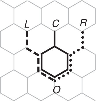
Figure 3: Different kind of steps of the random walk of a string.

The array of strings is characterized only by its density $\rho=1/\ell$ and the elastic line tension $g$ of the strings. The interaction between the strings consists only of the non-crossing constraint and thus introduces no additional energy scale. The configurations of a single directed string are characterized by its position function $x_{i}(z)$ since overhangs are forbidden. The reduced energy of all strings is then

$$\frac{H_{l}}{T_{l}}=\sum_{i}\int dy\,\frac{g}{2T_{l}}\left(\frac{dx_{i}}{dy}\right)^{2}.$$ (6)

First, we determine the line tension $g$ from a simple random walk argument. If $\bar{x}$ denotes the mean string position, then the total mean squared displacement of a string of length $L=\sqrt{3}aM$ along the $y$-direction (after $M$ steps), with $a$ the triangular lattice constant, must be

$$\sum_{i=1}^{M}\langle(x_{i}-\bar{x})^{2}\rangle=LT_{l}/g$$ (7)

in order to be consistent with the result of the continuum model of Eq.(6). Here $x_{i}=-a,\;0,\;+a$ are the three possible transversal steps. The different kind of steps correspond to the paths $OL$, $OC$ and $OR$ shown in Fig. 3. The corresponding probabilities for the steps can be expressed in terms of the weights of the occupied non-vertical bonds as

$$p_{L}=\frac{z_{2}^{2}}{(z_{1}+z_{2})^{2}},\;p_{C}=\frac{2z_{1}z_{2}}{(z_{1}+z_{2})^{2}},\;p_{R}=\frac{z_{1}^{2}}{(z_{1}+z_{2})^{2}}.$$ (8)

The mean position after one step is

$$\bar{x}=(p_{R}-p_{L})\,a=\frac{z_{1}-z_{2}}{z_{1}+z_{2}}a.$$ (9)

Thus, after $M$ steps, the variance of the transverse wandering around the mean position is

$$\sum_{i=1}^{M}\langle(x_{i}-\bar{x})^{2}\rangle=L\frac{2}{\sqrt{3}\,(2+\eta+\eta^{-1})}a,$$ (10)

where $\eta=z_{1}/z_{2}$, yielding the line tension

$$\frac{g}{T_{l}}=\frac{\sqrt{3}\,(2+\eta+\eta^{-1})}{2a}.$$ (11)

The mean density of strings depends also on the dimer weights of the non-vertical bonds. It can be computed exactly with the result Nienhuis+84 ; yokoi+86

$$\rho=\frac{2}{\pi a}\arcsin\left[\frac{(z_{1}+z_{2})^{2}-1}{4z_{1}z_{2}}\right]^{1/2},$$ (12)

for $z_{1}+z_{2}>1$. For $z_{1}+z_{2}\leq 1$ the density vanishes kasteleyn1 , corresponding to a Kasteleyn or commensurate-incommensurate transition. For the isotropic TIAF, one has $z_{1}=z_{2}=1$ and $\rho=2/(3a)$.

Before we introduce the relation between the string displacement and the height profile, and a corresponding continuum description, it is instructive to focus on the free energy of the string array. This will allow for an independent check of our random walk description. Moreover, from the free energy one can determine the elastic constants on large length scales which are needed for the proper continuum model.

Actually, the density of strings is determined by the densities $\rho_{1}$, $\rho_{2}$ of non-vertical dimers with weights $z_{1}$, $z_{2}$, respectively. This can be seen from the fact that along a cut perpendicular to the string direction each non-vertical dimer corresponds to one string. It follows from Eq. (4) that

$$\rho_{i}=\frac{z_{i}}{N}\frac{\partial\log Z_{D}}{\partial z_{i}}\,,$$ (13)

for $i=1$, $2$, where the number of triangular lattice sites, $N$, equals the total number of dimers. The string density then reads

$$\rho=\frac{\rho_{1}+\rho_{2}}{a}\,.$$ (14)

Now we change variables from $z_{1}$, $z_{2}$ to $\eta=z_{1}/z_{2}$ and $\tilde{\rho}=\rho a$, see Eq.(12). Since $z_{1}\partial\eta/\partial z_{1}+z_{2}\partial\eta/\partial z_{2}=0$, and using Eq.(12), we have

$$z_{1}\frac{\partial}{\partial z_{1}}+z_{2}\frac{\partial}{\partial z_{2}}=\frac{1+\eta^{2}+2\eta\cos(\pi\tilde{\rho})}{\pi\eta\sin(\pi\tilde{\rho})}\frac{\partial}{\partial\tilde{\rho}}\,.$$ (15)

This allows us to derive a differential equation for the free energy density of the dimers,

$$f_{D}=-\frac{2\log Z_{D}}{\sqrt{3}Na^{2}}$$ (16)

as a function of the parameters $\eta$, $\rho$ of the string system. $f_{D}$ fulfills the equation

$$\frac{\partial f_{D}}{\partial\rho}=-\frac{2\pi}{\sqrt{3}}\frac{\eta\rho\sin(\pi a\rho)}{1+\eta^{2}+2\eta\cos(\pi a\rho)}.$$ (17)

Integrating the latter expression yields the exact result for the lattice string model. In the continuum limit $a\to 0$, the result simplifies to

$$f_{D}=-\frac{\pi^{2}}{3}\frac{2a}{\sqrt{3}(2+\eta+\eta^{-1})}\,\rho^{3}\,.$$ (18)

There is an alternative and simple approach to obtain the free energy in the continuum limit. The strings can be regarded as the world lines of free fermions in one dimension Pokrovsky+79 . The non-crossing condition is then implemented automatically by the Pauli principle. In the limit of infinitely long strings, the ground state energy density of the fermions equals the free energy density of the strings if the fermion mass is mapped to the line tension $g$ and $\hbar$ to the temperature $T_{l}$. From the expression for the ground state energy of one-dimensional free fermions follows immediately the reduced free energy density of the strings,

$$f_{l}=f_{1}\rho+\frac{\pi^{2}}{6}\frac{T_{l}}{g}\rho^{3}\,,$$ (19)

where $f_{1}$ is the reduced free energy (per length) of a single string, and the last term is generated by the reduction of entropy due to the non-crossing condition. A direct comparison of the free energies of Eqs.(18) and (19) is not possible since the number of strings varies with the dimer coverings although the number of dimers is fixed. Only the mean density of strings is fixed. Hence, one has to consider the grand potential density $j$ for the string system which follows easily from the free energy density,

$$j=f_{l}-\mu\rho=-\frac{\pi^{2}}{3}\frac{T_{l}}{g}\rho^{3}\,,$$ (20)

where $\mu=\partial f_{l}/\partial\rho$ is the chemical potential (per string length). Comparing Eq.(18) and Eq.(20), we see that $f_{D}=j$ exactly for the expression of the line tension which we obtained above from an independent random walk argument, see Eq.(11). Thus in the continuum limit the ground states of the TIAF and the dimer model can be described as free fermions with their mass determined by our simple random walk argument on the lattice.

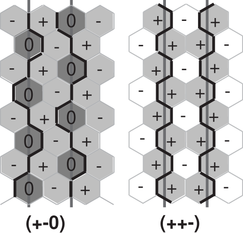
Figure 4: Two different flat states, with the corresponding sublattice magnetizations of the isotropic TIAF indicated below.

Now we turn to the structural properties of the string lattice. The most ordered state consists of straight (“flat”) strings which do not wander transversally. Depending on the string density there are different commensurate and incommensurate states possible. For the discussion of the flat states we focus on the state with a maximal density of $\rho=2/(3a)$ which corresponds to the most interesting case of isotropic couplings for the TIAF. In this case there are two non-equivalent classes of flat strings which are not related by shifts by a nearest-neighbor vector of the triangular lattice, see Fig. 4. These classes translate directly to different ordered spin states which are characterized by their sublattice magnetizations. One state, $(+-0)$, is obtained by orienting two sublattices uniformly but opposite while the third sublattice has the same number of $+$ and $-$ spins, leading to zero magnetization. This, on average, locks the straight strings on the sublattice with zero magnetization. Since each of the three sublattices can be chosen as the one with zero magnetization, equivalent flat string states are related by a shift of $a/2$. The other state, $(++-)$, has up spins on two sublattices and down spins on the other sublattice which places the non-vertical dimers on straight strings that are locked symmetrically between the two sublattices with equal magnetization.

The displacement $u$ from flat strings is determined by the original height profile $h$ of the corresponding dimer covering. Since only non-vertical dimers are conserved under the subtraction of the reference covering, we will defined $u$ for each non-vertical bond of the hexagonal lattice. If a bond is occupied by a string segment, then $u$ measures the normal distance between the corresponding flat string and the center of the segment, cf. Fig. 2(c). Since a shift of the height $h$ by $3$ corresponds to a string translation by the mean string distance $\ell$, the displacement on each non-vertical bond is given by $u=\ell\bar{h}/3+u_{0}$ where $\bar{h}$ is the coincident (original) height of the two hexagonal plaquettes which are joined by the non-vertical bond, see Fig. 2(a). $u_{0}$ is a global offset of the flat string lattice. For $u_{0}=n\,a/2$, $n\in{\mathbb{Z}}$, the class $(++-)$ is chosen while $u_{0}=a/4+n\,a/2$ selects $(+-0)$. This definition of $u$ is equivalent to the height profile introduced by Zeng and Henley Zeng+97 by averaging over the three sites of every triangle in order to obtain a coarse-grained height on the center of the triangles.

After a coarse-graining over length scales large compared to the lattice constant, one obtains a continuous field $u({\bf r})$ which allows to write the effective free energy of long-wavelength fluctuations of the string lattice in the form of a continuum elastic energy,

$$\frac{{\cal F}_{\rm el}}{T_{l}}=\int d^{2}{\bf r}\left\{\frac{c_{11}}{2}(\partial_{x}u)^{2}+\frac{c_{44}}{2}(\partial_{y}u)^{2}+V_{L}(u)\right\}$$ (21)

with compression $c_{11}$ and tilt $c_{44}$ modulus. The tilt modulus is fixed by the line tension $g$ as $c_{44}=(g/T_{l})\rho$. The compression modulus on asymptotically large length scales is affected by the entropic repulsion between strings and has to be determined in a macroscopic way. The compressibility of the lattice is given by the second derivative of the free energy density with respect to the mean distance $\ell=1/\rho$ between the strings landau1 , which leads to the result

$$c_{11}=\ell\frac{\partial^{2}}{\partial\ell^{2}}[\ell f_{l}(\ell)]=\pi^{2}\frac{T_{l}}{g}\rho^{3}\,,$$ (22)

where we have used Eq.(19). $V_{L}(u)$ is a periodic potential which reflects the discreteness of the lattice and favors an ordered phase with flat strings. Since equivalent flat states are related by shifts of all straight strings by $a/2$ and since $u=\ell h/3+u_{0}$, the locking potential must have the form footnote1

$$V_{L}=-v\cos\left(\frac{4\pi}{a}(u-u_{0})\right)=-v\cos\left(\frac{4\pi}{3}\frac{\ell}{a}h\right)$$ (23)

with $v>0$. If $\sqrt{c_{11}c_{44}}>2\pi/a^{2}$ the string lattice is sufficiently stiff and the potential $V_{L}$ is relevant (under renormalization) so that the strings lock into one of the flat states. Interestingly, $\sqrt{c_{11}c_{44}}=\pi/\ell^{2}$ is independent of the line tension, and the locking potential is relevant for $\ell<a/\sqrt{2}$. However, the minimal string separation is $\ell=3a/2$ (corresponding to isotropic dimer weights), and hence $V_{L}$ is irrelevant at all possible densities.

However, if there are additional interactions present which increase the stiffness of the string lattice, the lock-in potential might become relevant. In fact, we will see below that a coupling of many TIAF can render the periodic pinning relevant. Therefore, it is important to determine the consequences of the lock-in potential for the spin configurations, which depend on the sign of that potential. To do so, we recall that the offset $u_{0}$ selects the lattice positions of the strings in the flat states. It has to be determined from additional information which is in the present case provided by spin configurations which correspond to flat strings and small fluctuations around the locked-in states. Thus, we focus now on the isotropic TIAF so that the possible classes of flat states are those shown in Fig. 4. If one switches between the two classes, $u_{0}$ shifts by $a/4$ and thus the sign of $V_{L}$ changes. The sign can be determined as follows.

The systems selects the class with the largest entropy, i.e., with the maximal number of configurations which yield at arbitrary large ${\bf r}$ still a finite displacement $\langle[u({\bf r})-u({\bf 0})]^{2}\rangle_{\text{flat}}\sim\text{const.}$, where the displacement is measured relative to the respective flat state. For large systems, the entropy of such macroscopically flat states can be estimated from the number of string configurations on the hexagonal lattice for which each string fluctuates in a tube of width $\ell$ about its straight reference position, i.e., $|u|\leq\ell/2=3a/4$ for each non-vertical dimer footnote2 . This puts a strong constraint on the spin states since a flip of a single flippable spin (a spin with 3 up and 3 down spins as neighbors) shifts a string by the hexagonal plaquette on which the spin sits. In the class $(+-0)$ the spins on one sublattice (dark grey in Fig. 4) can assume any of the $2^{N/3}$ possible states where $N$ is the number of triangular lattice sites. The maximal displacement of $u=3a/4$ is obtained if spins on the other two sublattices are also flipped with respect to the perfectly ordered state $(++-)$ which, however, is possible only for $1/2^{3}\times 2N/3$ sites since the $3$ neighbors on the fully flippable sublattice must have the same orientation as the spin to be flipped in order to have directed and non-crossing strings. This yields $2^{N/3+N/12}=\exp(0.2888\,N)$ configurations. For the fluctuations in class $(++-)$ all spins on one sublattice (white in Fig. 4) are frozen. The sites of the other two sublattices can be divided into $N/12$ “rings”, each of $6$ plaquettes centered about a frozen site, and $N/6$ extra plaquettes between the rings. Due to the constraints on the strings, each ring permits only $18$ spin states. For a given spin state on all rings, the extra plaquettes can only flip if its $3$ neighboring spins located on rings point up, which occurs with probability $(13/18)^{3}$. Thus there are $18^{N/12}\times 2^{(13/18)^{3}N/6}=\exp(0.2844\,N)$ configurations. We conclude that entropy favors flat states of the class $(+-0)$ and one has to set $u_{0}=-a/4$ as shown in Fig. 2 (c), i.e., $V_{L}(u)=v\cos(4\pi u/a)$ with positive amplitude $v$.

III.3 Spin-spin correlations

In this section, we are going to apply the above framework to the spin correlations of the TIAF model at zero temperature. We concentrate on isotropic couplings since otherwise the system is ordered. We have seen that the ground state manifold of the isotropic TIAF can be regarded as the configuration space of a string lattice. Based on the irrelevance of lattice pinning effects, one can expect from the effective elastic description of Eq.(21) an algebraic decay of correlations which is characteristic for such kind of two-dimensional systems. In fact, this corresponds to the exact result found by Stephenson Stephenson70 .

The displacement correlations of the string lattice can be easily computed for large ${\bf r}$ from Eq.(21) with the result

$$\langle(u({\bf r})-u({\bf 0}))^{2}\rangle=\frac{1}{\pi}\frac{1}{\sqrt{c_{11}c_{44}}}\log\left(\frac{r}{a}\right)\,.$$ (24)

So far, we have constructed the string displacement field and the height profile from a given dimer covering of the hexagonal lattice. Although the dimer covering in turn is uniquely determined by the corresponding spin state, we have not yet established a direct relation between the spin variables $\sigma_{i}$ and the displacement field $u$. We will first express the spin variable in terms of the height profile. For a given spin state, we chose one up spin and consider its site as the point of origin with height $h=0$. The construction of the dimer covering from the spin state means that the height on all other sites is then fixed since parallel (antiparallel) spins imply a height change by $+2$ ($-1$) from site to site if the down pointing triangles are traversed clockwise. If a single spin is flipped, the height on that site changes by $\pm 3$. From this is it clear that the height profile can locally be changed by $6$ without affecting the spin state. However, a spin flip with such a change in $h$ leads out of the ground state manifold. Allowing for this excitations, the height profile is no longer single-valued. This induces topological defects which are vortex-anti-vortex pairs in form of two triangles, each having three parallel spins, see Fig. 5. Along a closed curve around a single (anti-)vortex the height changes by $6$. One easily proves that the above constraints are met by the spin-height relation

$$\sigma_{i}=\cos\left(\mathbf{q}\cdot\mathbf{r}_{i}+\frac{\pi}{3}h_{i}\right)=\pm 1\,,$$ (25)

with $\mathbf{q}=(4\pi/(3a),0)$ and the triangular lattice sites ${\bf r}_{i}$. The relation to the string displacement field is then given by the coarse grained relation $\bar{h}=3(u-u_{0})/\ell$ with $\ell=3a/2$ in the isotropic case considered here. Using these relations, the spin-spin correlation function can be written as

$$\langle\sigma_{i}\sigma_{j}\rangle=\cos\left[\frac{4\pi}{3a}(x_{i}-x_{j})\right]e^{-\frac{1}{2}\frac{\pi^{2}}{\ell^{2}}\langle[u({\bf r}_{i})-u({\bf r}_{j})]^{2}\rangle}\,,$$ (26)

where we have used the fact that $u({\bf r})$ is Gaussian and that there are no topological defects at $T=0$. From Eq.(24) and $\sqrt{c_{11}c_{44}}=\pi/\ell^{2}$ it immediately follows that

$$\left\langle\sigma_{i}\sigma_{j}\right\rangle=\cos\left[\frac{4\pi}{3a}(x_{i}-x_{j})\right]\frac{1}{|{\bf r}_{i}-{\bf r}_{j}|^{\eta}}$$ (27)

with $\eta=1/2$ which is in agreement with the exact result Stephenson70 . The anisotropy factor depends here only on the $x$-coordinates of the spins since the $x$-axis had been chosen to coincide with one of the triangular lattice directions.

Finally, we consider the height correlations for general anisotropic dimer weights. These correlations have been studied in the context of the triangular SOS model some time ago Bloete+82 ; Nienhuis+84 . In those works, the correlations were obtained from four-spin correlations of the TIAF in the isotropic case, and in terms of the Pfaffian method for the anisotropic situation. In contrast, here we present a simple derivation of the correlations based on our effective elastic description of the string lattice. The mean squared height difference between two distant positions increases logarithmically as the string displacement does. The coefficient $K$ measures the large-scale stiffness of the height profile,

$$\langle(h({\bf r})-h({\bf 0}))^{2}\rangle=\frac{1}{\pi K}\log\left(\frac{r}{a}\right)\,,$$ (28)

By making use of the relation between the height profile and the string displacement field, one easily gets

$$K=\frac{\ell^{2}}{9}\,\sqrt{c_{11}c_{44}}=\frac{\pi}{9}\,,$$ (29)

which is independent of the dimer weights $z_{1}$ and $z_{2}$. This remarkable universality was found already in the exact solution of the dimer model in Refs. Bloete+82, ; Nienhuis+84, , but the physical reason for that remained unclear. Our interpretation of the stiffness $K$ as the geometric mean of the two elastic constants of the string lattice can explain the universality. By changing the dimer weights, one tunes both the string density and the string tension $g$. Naively, one would expect that an increasing $g$ would render the height profile stiffer. However, there is also a reduction of the entropic repulsion between the strings which accompanies the reduction of string fluctuations. Interestingly but effects act together as to generate universality since $c_{44}\sim g$, $c_{11}\sim 1/g$ and the density dependent relation between $h$ and $u$.

III.4 Finite temperature

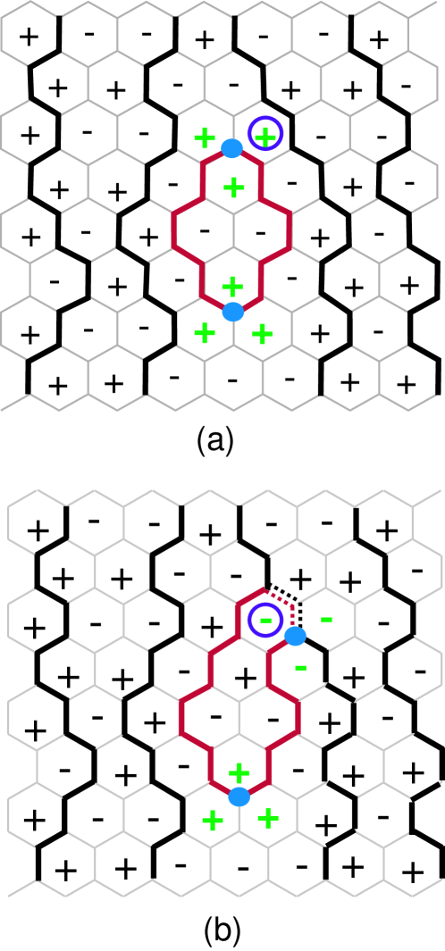
Figure 5: (color online) (a) Vortex-anti-vortex pair connected by a string loop. (b) Loop connected to a string as to generate a non-directed string. This configuration is obtained from the one in (a) by flipping a single spin (encircled) which costs no energy.

For the TIAF at finite temperatures, the mapping from spin states to string lattices can still be applied. The strings remain non-crossing, since each triangle can have only one or three frustrated bonds. However, the triangles with three frustrated bonds are excitations that generate topological defects, see Fig. 5(a). Two defects form a pair that spans a string loop which is confined between the strings, i.e., strings cannot cross loops. However, loops can attach to strings resulting in non-directed strings, see Fig. 5(b). The fugacity for the lowest energy single-spin excitations is $e^{-4J/T}$. The quasi-long-range-order of the $T=0$ phase is destroyed if the defect pairs can unbind. This will happen at sufficiently weak string lattice stiffness. Actually, the critical stiffness for that is $\sqrt{c_{11}c_{44}}=2\pi/\ell^{2}$ and hence by a factor of two larger than the actual stiffness corresponding to the TIAF at $T=0$. Hence topological defects are always a relevant perturbation but they can occur only for $T>0$ where the fugacity is finite, leading to exponentially decaying spin correlations. Thus the system does not show a Kosterlitz-Thouless transition by tuning the temperature.

IV Stacked (2+1)D Ising model

After we have introduced the description of the frustrated 2D TIAF in terms of fluctuating strings, we shall apply this mapping now to study the $(2+1)$-dimensional stacked TIAF which consists of ferromagnetically coupled TIAF layers, see Eq.(1). As in the 2D system, the in-plane frustration is expected to have strong influence on the underlying physics due to the Ising symmetry. Actually, the behavior is independent of the interaction along the stacking direction, whether it is ferro- or antiferromagnetic. Experimentally, the stacked model is a reasonable description of triangular cobalt antiferromagnets of the type ACoX₃ where A is an alkali metal and X a halogen atom Collins+97 . For these magnets, a strong crystal field splitting leads to an effective spin $1/2$ state with the moment oriented along the stacking direction. In these compounds the in-plane exchange coupling $J_{\|}$ is small compared to the inter-plane coupling $J_{\perp}$. The increased dimensionality of the stacked system reduces the degeneracy of the ground state so that the entropy per spin vanishes at $T=0$ and ordering at even finite-temperature might be possible. This is also suggested by the following argument Blankschtein+84 . Each ground state of the 2D TIAF yields a ground state of the stacked system if all spins are aligned along the stacking direction, i.e., the configuration in each layer is identical. Hence, at $T=0$ the spin correlation function cannot decay in-plane faster than that of the 2D system. However, one might wonder if the system can gain entropy by introducing domain walls parallel to the layers which would destroy the order along the stacking direction. The average energy cost for such a wall is at least

$$E_{\rm dw}\sim 2J_{\perp}\int_{0}^{N^{1/3}}\frac{2\pi r}{\sqrt{r}}dr\sim N^{1/2}$$ (30)

where $N$ is the total number of spins of the 3D system and we used the power law of Eq. (27). This has to be compared to the entropy gain which growth only $\sim(1/3)\log N$ since the wall can be placed at any of the $N^{1/3}$ layers. This naive argument suggests the absence of domain walls at $T=0$, and order along the stacking direction. Moreover, as we will see more clearly below, the huge in-plane degeneracy can actually induce order even in-plane, a phenomenon known as order from disorder Villain+80 .

The stacked TIAF has been studied first by Blankschtein et al Blankschtein+84 . Their results based on the LGW approach and Monte Carlo simulations suggested the existence of two different ordered phases and a XY-like transition into the paramagnetic phase. The LGW Hamiltonian was constructed for the large scale fluctuations about the two minimal energy modes with wave vectors ${\bf Q}_{\pm}=(\pm 4\pi/3,0)$, leading to a 3D XY model with a 6-fold symmetry breaking term,

$$H_{{\rm LGW}}(\psi) = \int d^{3}{\bf r}\Big{\{}\frac{1}{2}|\nabla\psi_{0}|^{2}+\frac{r}{2}|\psi_{0}|^{2}+u_{4}|\psi_{0}|^{4}$$ (31)

$$\,+\,u_{6}|\psi_{0}|^{6}+v_{6}|\psi_{0}|^{6}\cos\left(6\phi\right)\Big{\}},$$

for the complex order parameter $\psi({\bf r})=\psi_{0}\,e^{i\phi}$. Since for $p\gtrsim 3.4$ the symmetry breaking term is irrelevant in 3D [Aharony+86, ], the LGW theory predicts for the transition to the paramagnetic phase XY universality Blankschtein+84 ; Netz+berker . The sign of $v_{6}$ is not fixed in this approach, and hence two ordered phases with a relevant symmetry breaking term are possible in principle (see below for the two types of ordering). In fact, the two corresponding phases were observed with increasing temperature in the Monte Carlo simulations in Ref. Blankschtein+84, . However, more recent simulations indicated the existence of only one ordered phase which corresponds to the one found in Ref. Blankschtein+84, at higher temperatures only Matsubara+87 ; Kim+90 ; Nagai+94 ; Plumer+95 ; Moessner+01b . This conclusion is also supported by a hard-spin mean field theory Akguc+95 . There is also a controversy about the nature of the transition to the paramagnetic state. While the simulations of Heinonen et al. indicate tricritical behavior Heinonen+89 , a histogram Monte Carlo analysis supports XY-like behavior Bunker+93 . These conflicting results have to be viewed against the background of Coppersmith’s work Coppersmith85 . She argued that the above mentioned LGW approach is not reliable since it ignores the geometric frustration and hence does not yield the correct low temperature state.

In the following, by making use of the string mapping established in the preceding section, we provide a microscopic derivation of the LGW action for the stacked TIAF. This will allow us to discuss the nature of the ordered phase and the transition to the paramagnetic state. In each layer, we relate the spin variables $\sigma_{ik}$ to a height profile $h_{ik}$ as in the preceding section so that the relation of Eq. (25) holds for every layer. Then the intra-layer coupling can be written as

$$\sigma_{ik}\sigma_{jk}=-\cos\left[\frac{\pi}{3}\left(h_{ik}-h_{jk}+\eta_{ij}\right)\right]$$ (32)

with a shift $\eta_{ij}=+1$ for the bond directions $(a,0)$ and $\eta_{ij}=-1$ for the directions $(a/2,\pm\sqrt{3}a/2)$. Next, we have to define how the height should change along the stacking direction. Since $h_{ik}$ changes by $\pm 3$ for a spin flip, we set along the column passing through the origin of each layer $h_{0k}=0$ $(3)$ if $\sigma_{0k}=+1$ $(-1)$, where $k$ numbers the layers. According to this rule, the inter-layer coupling reads

$$\sigma_{ik}\sigma_{ik+1}=-\cos\left[\frac{\pi}{3}\left(h_{ik}-h_{ik+1}\right)\right]\,.$$ (33)

Now, the height profile can again be interpreted as the displacement field of strings, which now form a 3-dimensional lattice. Hence, it is expected to more stable against fluctuations, and spin order will occur. However, the periodic couplings of the displacement field allow for topological defects which eventually drive the system into the paramagnetic state. Even in the presence of defects, the picture of non-crossing strings remains valid since a triangle can have either 1 or 3 frustrated bonds. When introducing continuous fields, the lock-in potential of Eq.(23) has to be included as to reflect the original discreteness of the height which reads $h_{ik}=3(u_{ik}-u_{0})/\ell$ in terms of the string displacement $u_{ik}$. Hence, we obtain the reduced 3D string Hamiltonian

$$\!\!\!\!\!\!\!\!\!\!H_{S}\!\! = \!\!-\tilde{K}_{\|}\!\!\sum_{\langle ij\rangle,k}\!\cos\left[\frac{\pi}{\ell}(u_{ik}-u_{jk}+\eta_{ij}a/2)\right]$$

$$- \!\!\tilde{K}_{\perp}\!\sum_{i,k}\!\cos\left[\frac{\pi}{\ell}(u_{ik}\!-\!u_{ik+1})\right]+v\!\sum_{i,k}\!\cos\left[\frac{6\pi}{\ell}u_{ik}\right]$$

with couplings $\tilde{K}_{\|}=J_{\|}/T$, $\tilde{K}_{\perp}=J_{\perp}/T$ and mean string separation $\ell=3a/2$. Here $v>0$ due to the entropy argument at the end of Section III.2. The in-plane shift $\eta_{ij}$ reflects frustration since $\sum\eta_{ij}=3$, where the sum runs over the bonds of a down pointing triangle. Since in the discrete version the $u_{ik}$ can vary over the bonds only by $+a$ or $-a/2$, the energy is minimized for a non-uniform change of $u_{ik}$ along the triangles. This is distinct from a priori continuous field of an antiferromagnetic XY model on a triangular lattice whose oriented uniform change defines a helicity, giving rise to an additional ${\mathbb{Z}}_{2}$ symmetry leedh1 . Hence, the latter $XY$ model exhibits a Ising transition because of the ${\mathbb{Z}}_{2}$ symmetry breaking of the ground states leedh1 . However, in the present case, the non-crossing restriction for the strings, originating from the geometrical frustration, prohibits this extra symmetry breaking.

Thus the stacked Ising model of Eq.(1) maps to a stack of planar lattices of non-crossing strings which is described by a (2+1)D frustrated XY model with a 6-fold clock term. Interestingly, this provides a microscopic derivation of the LGW theory Blankschtein+84 if the string displacement $u$ is identified with the phase $\phi$ of the order parameter via $\phi=\pi u/\ell$. However, our effective model differs from the LGW theory in two important points: (i) the in-plane XY coupling is frustrated and (ii) there is a topological constraint on $\phi$ since $u$ is restricted by the non-crossing condition. The latter point will lead to an entropicly increased phase stiffness on large length scales.

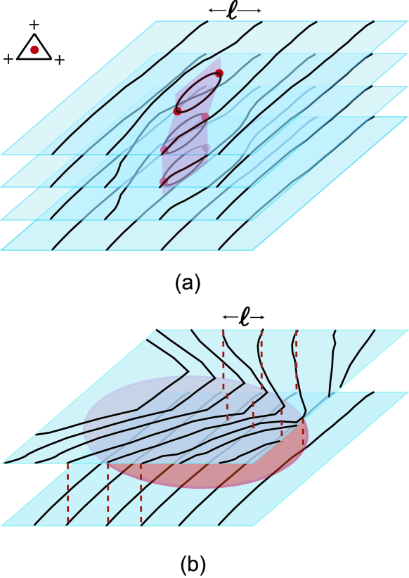
Figure 6: (color online) Different type of topological defects. (a) vortex-anti-vortex pairs in the layers form vortex loops perpendicular to the planes. (b) vortex loop parallel to the planes which borders the mismatch regions in which the strings in two adjacent planes are shifted by $2\ell$.

With the model of Eq. (IV) at hand, we can analyze the ordering mechanism and the transition to the paramagnetic phase. The latter transition is driven by topological defects which are generated by thermal fluctuations. It is well known that the XY coupling allows for defect loops across which $\phi$ changes by $2\pi$. These defects are superpositions of two kind of loops [cf. Fig. 6]: fully frustrated triangles with all spins aligned form in-plane vortex-anti-vortex pairs, which can be viewed as a string forming an in-plane loop. Together with other pairs in the neighboring layers they form defect loops oriented perpendicular to the planes, cf. Fig. 6(a). Another type of defect loops is oriented parallel to the layers. They arise as the boundaries of 2D areas across which strings in adjacent planes are shifted by $2\ell$, cf. Fig. 6(b). For the universality class of the transition to the ordered state it is important to take into account the stacked nature of the $(2+1)$D XY model and the $6$-fold clock term. In turns out that the stacking is irrelevant since the layers cannot decouple independently from the vortex unbinding transition within the layers. This is due to the fact that unbinding of defects oriented parallel to the layers can occur only at a critical value for the effective coupling $K_{\|}$ which is by factor of $1/8$ below that for the in-plane dissociation of vortices Korshunov90 . In addition, a $6$-fold clock term is known to be irrelevant at the XY critical point under renormalization if $p\gtrsim 3.4$ [Aharony+86, ]. Hence we conclude that the transition from the paramagnetic phase to an ordered state must be in the 3D XY universality class.

In the following, let us discuss the property of the ordered phase. In the latter phase, the XY couplings of Eq. (IV) can be expanded in $u_{ik}$, and in the continuum limit each layer is described by Eq. (21) with an additional harmonic inter-layer coupling. Moreover, the $6$-fold clock is relevant, and the strings are locked into a flat state with spin order whose nature depends on the form of the locking potential. In order to compare our approach with the LGW theory Blankschtein+84 , we discuss potential ordered states. As we have seen in Section III.2, there are two classes of flat strings. They differ by their value of the shift $u_{0}$ in the lock-in potential $V_{L}(u)$. After going over from the discrete field $u_{ik}$ to a coarse-grained description with a continuous field $u({\bf r})$, the coarse-grained spin variable can be written as

$$\sigma({\bf R}_{jk})=\cos\left(\mathbf{Q}\cdot\mathbf{R}_{jk}+\frac{2\pi}{3a}(u({\bf R}_{jk})-u_{0})\right)\,,$$ (35)

where ${\bf R}_{jk}$ are the 3D lattice sites and ${\bf Q}=(4\pi/(3a),0,0)$. For flat strings, the coarse-grained field $u({\bf r})$ is zero on average, and the global shift $u_{0}$ determines the sublattice magnetizations. For the first state, cf. left part of Fig. 4, $u_{0}=-a/4$, and there is an additional shift of $\pi/6$ in Eq.(35), leading to the sublattice magnetizations $\langle\sigma\rangle=(\frac{\sqrt{3}}{2},-\frac{\sqrt{3}}{2},0)$. For the second state, cf. right part of Fig. 4, $u_{0}=0$, one has the sublattice magnetizations $\langle\sigma\rangle=(1,-\frac{1}{2},-\frac{1}{2})$ since ${\bf QR}_{jk}=0$, $4\pi/3$, or $-4\pi/3$ on the three sublattices. Hence all sublattices are at least partially ordered. Since our entropy argument lead to $u_{0}=-a/4$, the first state with one fully disordered sublattice should set up the ordered phase at all temperatures which appears to be consistent with more recent simulations.

How can this ordering be reconciled with the fact that each ground state of the highly degenerate and hence disordered 2D TIAF is also a ground state of the stacked model when all spins are aligned along the stacking direction? This is the point where the mechanism of order from disorder comes into play. As we have seen at the beginning of this section, the formation of domain walls parallel to the layers is energetically not favorable. However, the system can gain entropy by flipping single (so called flippable) spins in a single layer which does not cost energy within the layer. Due to the huge ground state degeneracy there are many configurations which just differ in their orientation of flippable spins. Hence, a subset of all the 2D ground states is selected which allows for those single spin flips. This explains the existence of the found ordered state since it is composed only of an appropriate subset of all 2D ground states which on average has one sublattice disordered. The spins on this disordered sublattice form chains along the stacking directions which are decoupled from each other at low temperatures, and hence should behave as individual 1D Ising spin chains. At sufficiently low temperatures, the stacked system is thus expected to show excitations which are 1D Ising-like. This conclusion is consistent with multi-spin Monte Carlo simulations of the specific heat at low temperatures Kim+90 .

V Quantum frustrated model

Having established the relation of the $(2+1)$-dimensional TIAF to a lattice of fluctuating strings with topological defects, we now will apply this relation to the $2$-dimensional TIAF in a transverse magnetic field. The Hamiltonian of this model is given in Eq. (2). The transverse field introduces simple quantum dynamics to the highly degenerate critical state of the classical TIAF. Due to the general relation between 2D quantum spin systems and 3D classical Ising spin models suzuki1 , one can expect from the results for the stacked TIAF quantum order arising from the interplay of quantum fluctuations and geometric frustration. The existence of a quantum ordered state was suggested in recent works on the basis of a LGW theory moessner1 , a kink model Mostovoy+03 , and simulations Isakov+03 .

The exact mapping from the 2D quantum TIAF to a classical stacked Ising system is provided by Suzuki’s theorem which states that the partition function of the quantum system can be written as suzuki1

$$Z = \mathrm{Tr}\;\exp\left\{-\frac{J}{T}\sum_{\langle i,j\rangle}\sigma_{i}^{z}\sigma_{j}^{z}+\frac{\Gamma}{T}\sum_{i}\sigma_{i}^{x}\right\}$$ (36)

$$= \lim_{n\to\infty}\left[\!\frac{1}{2}\sinh\left(\frac{2\Gamma}{nT}\right)\right]^{\frac{nN}{2}}\!\!\sum_{\{\sigma_{ik}\}}\!\exp\Big{\{}\!-\frac{J}{nT}\!\!\sum_{\langle i,j\rangle,k}\!\sigma_{ik}\sigma_{jk}$$

$$+ \frac{1}{2}\log\coth\left(\frac{\Gamma}{nT}\right)\sum_{i,k}\sigma_{i,k}\sigma_{i,k+1}\Big{\}},$$

where $\sigma_{ik}=\pm 1$ are classical Ising variables which are defined on a stacked system of $n$ antiferromagnetic triangular lattices, and the second index $k=1,\ldots,n$ refers to the layer number. Hence, in the relevant limit of large $n$ the quantum system is described by the Hamiltonian of the stacked TIAF of Eq. (1) with the couplings $J_{\|}$ and $J_{\perp}$ replaced by a infinitesimal small in-plane coupling $\tilde{K}_{\|}=J/(nT)$ and a strong ferromagnetic inter-layer coupling $\tilde{K}_{\perp}=\frac{1}{2}\log(nT/\Gamma)$ which is controlled by the strength of the quantum fluctuations, i.e., the transverse field $\Gamma$. In analogy with the preceding section, the quantum system is hence described by a $(2+1)$D string lattice with the Hamiltonian of Eq. (IV). This suggests that, as for the classical 3D system, the transverse field Ising model must have an ordered phase at small transverse field and a quantum phase transition in the 3D XY universality class to a disordered state. This scenario was previously predicted from by the LGW approach. However, in contrast to the latter approach, our mapping of the quantum frustrated spin system to strings yields even the coupling constants of Eq. (IV) which is of utmost importance for the construction of the phase diagram.

V.1 Quantum critical point

First, let us focus on the quantum phase transition to the paramagnetic phase. The purpose of the following analysis is to estimate the location of the critical point and to show that the Trotter limit $n\to\infty$ can be carried out explicitly in our approach. It is useful to separate the partition function associated with the XY model of Eq. (IV) into a spin wave part and a vortex part. This can be done by making use of the fact that the planar model can be mapped to a simpler model proposed by Villain Villain75 . As was shown by Kleinert kleinert1 and in Ref. jose1, , in the partition function one can make the substitution

$$e^{\tilde{K}\cos(\phi)}\to c\!\sum_{m=-\infty}^{\infty}e^{-K(\phi-2\pi m)^{2}/2}\,,$$ (37)

where the right hand side is known as Villain coupling kleinert1 ; jose1 with a new $\tilde{K}$-dependent coupling $K$ . Both expressions become identical in the two limits of $\tilde{K}\to 0$ and $\tilde{K}\to\infty$ which are fortunately precisely the two cases arising from the Trotter limit $n\to\infty$. Then the coupling constant $K$ and the coefficient $c$ are given by

$$K=\tilde{K}, c=e^{K}\quad\text{for}\quad\tilde{K}\to\infty$$ (38)

$$K=\frac{1}{2\log(2/\tilde{K})}, c=\sqrt{2\pi K}\quad\text{for}\quad\tilde{K}\to 0$$ (39)

Hence, after taking the Trotter limit, the coupling constants of the equivalent Villain model both scale logarithmically with $nT$,

$$K_{\perp}=\frac{1}{2}\log\left(\frac{nT}{\Gamma}\right),\quad K_{\|}=\frac{1}{2}\frac{1}{\log(2nT/J)}\,.$$ (40)

Only for $T=0$, one can set $T\sim J/n$ so that for $n\to\infty$ the coupling $K_{\perp}$ remains finite, and the system shows 3D behavior. For any finite $T$, however, $K_{\perp}$ must diverge with $n$ and the system shows a 3D to 2D crossover with increasing length scales.

Knowing the coupling constants of the Villain model with decoupled spin wave and vortex parts for large $n$, we can go ahead and apply dimensional crossover scaling in order to make quantitative predictions about the location and universality of the quantum critical point. We start by eliminating $n$ from Eq. (40). From this we obtain the temperature independent relation

$$K_{\perp}=\frac{1}{4K_{\|}}-\frac{1}{2}\,\log\left(2\,\frac{\Gamma}{J}\right)$$ (41)

between $K_{\|}$ and $K_{\perp}$ which makes the parameter space one dimensional. The geometric mean of the coupling constants controls the stiffness of the XY system. It can be expanded in the relevant limit of small $K_{\|}$ as

$$\sqrt{K_{\|}K_{\perp}}=\frac{1}{2}\left[1-\log(2\Gamma/J)\,K_{\|}+{\cal O}(K_{\|}^{2})\right]\,,$$ (42)

where we used the relation of Eq. (41). The latter relation will be compared to a crossover scaling result which provides a quantitative description of the increase of the transition temperature of a layered (2+1)D XY model under the increase of the number of layers. Following closely the analysis in Refs. Ambegaokar+80, ; schneider1, , one obtains a relation between the 3D critical value $K_{\infty}^{c}$ for the in-plane coupling and the corresponding $K_{n}^{c}$ for a system of $n$ layers,

$$\frac{1}{n}\frac{K_{\infty}^{c}}{K_{n}^{c}}=\gamma\left(\frac{K_{\|}}{K_{\perp}}\right)^{1/2}\left(1-\frac{K_{\infty}^{c}}{K_{n}^{c}}\right)^{\nu}$$ (43)

with the critical exponent $\nu\approx 2/3$ of the 3D XY model and a numerical constant $\gamma$. For $n=1$ this relation yields at the 3D critical point with $K_{\|}=K_{\infty}^{c}$ the following expression for the geometric mean of the coupling constants,

$$\sqrt{K_{\infty}^{c}K_{\perp}} = \gamma K_{1}^{c}\left(1-\frac{K_{\infty}^{c}}{K_{1}^{c}}\right)^{\nu}$$ (44)

$$= \gamma K_{1}^{c}\left(1-\nu\frac{K_{\infty}^{c}}{K_{1}^{c}}+\dots\right)\,,$$

where we have expanded for $K_{\infty}^{c}\ll K_{1}^{c}$. For consistency, the latter expression should be of the same form as the expression in Eq. (42) at the quantum critical point with $\Gamma=\Gamma_{c}$ corresponding to $K_{\|}=K_{\infty}^{c}$. Indeed, both expressions are identical if one sets

$$\gamma=1/(2K_{1}^{c}),\quad 2\Gamma_{c}/J=e^{\nu/K_{1}^{c}}.$$ (45)

Hence, the location of the quantum critical point is determined by the critical value for the coupling of the 2D XY model on a triangular lattice. The standard Kosterlitz-Thouless argument for the vortex unbinding transition yields leedh1 in that case $K_{1}^{c}=2/\pi\times 2/\sqrt{3}$, leading to $\Gamma_{c}/J=1.24$. However, this scaling approach neglects renormalization effects due to the $6$-fold clock term and the non-crossing of strings which should provide a net increase of $\Gamma_{c}$. This is consistent with recent Monte Carlo studies which suggest $\Gamma_{c}/J\approx 1.65$ [Isakov+03, ].

V.2 Phase diagram

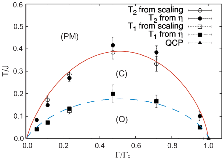
Figure 7: (color online) Phase diagram with the phase boundaries given by Eq. (46) with $b=0.98$ and Monte Carlo results of Fig. 1 in Ref. Isakov+03, . A critical phase (C) is separated by a boundary at $T_{c,2}$ from the paramagnetic phase (PM) and at $T_{c,1}=4/9\,T_{c,2}$ from an ordered phase (O).

Having established the existence of an ordered phase for $\Gamma<\Gamma_{c}$ at $T=0$, it is important to study the stability of this phase against thermal fluctuations. For finite temperatures, 2D XY physics should dominate at large length scales, and two Kosterlitz-Thouless transitions separating a critical phase at intermediate temperatures from the ordered and the paramagnetic state, respectively, are expected jose1 . In the following we will construct a quantitative phase diagram for the transverse field TIAF in the $\Gamma$-$T$-plane. The stability range of the phase with bound defects can be estimated from the crossover scaling formula of Eq. (43). Setting in the latter expression $K_{\|}$ to its critical value $K_{n}^{c}$ for a $n$-layer system, and using the scaling formula also at $n=1$ in order to relate $K_{\infty}^{c}$ to $K_{1}^{c}$ and the bare coupling ratio $K_{\perp}/K_{\|}$, we can derive an expression for the Kosterlitz-Thouless transition temperature $T_{c,2}(\Gamma)$ of the critical phase (C) which has only bound defects [see Appendix A for details],

$$\frac{T_{c,2}}{J}=b\,\frac{\Gamma}{\Gamma_{c}}\,\log^{\nu}\left(\frac{\Gamma_{c}}{\Gamma}\right)\,,$$ (46)

where $b$ is a numerical constant which is fixed by the (unknown) renormalization of $K_{\perp}$ and remains finite for $n\to\infty$. At large but finite $n$, for consistency, the renormalized effective coupling for the $n$-layer system must behave at as $K_{\perp}^{\rm eff}\sim(n/n_{c})^{3/5}$ with a characteristic number $n_{c}=bK_{1}^{c}(J/T)(\Gamma/\Gamma_{c})$ which is a measure for the strength of quantum fluctuations and characterizes the effective system size along the Trotter (“imaginary time”) axis. The spin correlation function in the critical phase (C) decays according to Eq. (27) with the exponent $\eta$ varying continuously between $\eta=1/4$ at $T_{c,2}$ and $\eta=1/9$ at a lower critical temperature $T_{c,1}$ which marks the transition to the ordered phase (O) jose1 . The correlation function exponent behaves discontinuously at $\Gamma=0$ where it is $\eta=1/2$ and at the quantum critical point where the 3D XY result $\eta\approx 0.040$ holds Zinn-Justin .

At the lower critical temperature $T_{c,1}$ there is a second Kosterlitz-Thouless transition to an ordered state where the clock-term in Eq. (IV) is relevant and locks the strings to the lattice. For a single layer, this transition occurs at the critical coupling $K_{1}^{c}=9/(2\pi)\times 2/\sqrt{3}$, see Ref. jose1, . The boundary of the ordered phase can be obtained analogously to that at $T_{c,2}$, yielding

$$T_{c,1}=\frac{4}{9}\,T_{c,2}\,.$$ (47)

Close to the quantum critical point both Kosterlitz-Thouless transition temperatures vanish $\sim(\Gamma_{c}-\Gamma)^{\nu}$ as expected from scaling. Fig. 7 compares our analytical results to recent Monte Carlo data for the phase boundaries, showing very good agreement across the entire range of $\Gamma$ if we set $b=0.98$ in Eq.(46). According to our analysis of the ordered phase for the stacked system in Section IV the quantum ordered phase (O) is characterized by the finite sublattice magnetizations $(\sqrt{3}/2,-\sqrt{3}/2,0)$. This type of order is consistent with recent simulations Isakov+03 .

VI Conclusion and Extensions

In this article, we have studied for a 2D Ising system the combined effect of classic geometric frustration and an ordering mechanism which either results from stacking many 2D system or by allowing for quantum dynamics from a transverse field. We have presented an exact relation between spin variables and the displacement field of a string lattice which we used to derive an effective Hamiltonian which was obtained previously only on the basis of a LGW approach. This allowed us to determine the nature of the ordered phase, the universality of the quantum phase transition to the paramagnetic phase, and the quantitative phase diagram at finite temperatures. To our knowledge, this is the first approach for the analyzed models which explicitly performs the Trotter limit $n\to\infty$ to obtain quantitative results for the transition temperatures. We have compared the so obtained phase diagram to predictions of recent simulations and found satisfying agreement. We related the spin model also to its dimer model representation and the resulting height profile description. Implementing a simple random walk argument for the strings, we could derive the exact free energy in the continuum limit which was known before only from a more complicated Pfaffian method. Our approach could also explain the physical reason for the previously found universality of the large-scale stiffness of the height profile in the presence of anisotropic bond weights.

For future extensions of our approach it is interesting to note that the string analogy applies independently of the form of the spin couplings. Interestingly, the mapping to strings should also be useful in the presence of quenched disorder when the system usually exhibits spin glass behavior. The behavior of a 2D string lattice with pinning sites emig1 suggests that in geometrically frustrated systems the spin glass correlation function Binder-Young-RMP $g_{SG}\left({\bf r}_{i}-{\bf r}_{j}\right)=\overline{<\sigma_{i}\sigma_{j}>^{2}}$ decays at least according to a power law, which implies that the spin glass phase is destroyed by the huge degeneracy from the geometric frustration. However, quenched disorder will induce topological defects, and a full analysis is more complicated. The situation is under better control for geometrically frustrated Ising systems with random dilution. The dilution sites act as pinning centers for the strings and topological defects do not arise from this type of disorder.

In the quantum frustrated system, though it is very hard to get a clear picture of how the transverse field and quenched disorder act together, one can try to make use of a method analogous with what Moessner et al. moessner1 used in discussing the existence of an ordered phase in clean quantum frustrated Ising systems. Moessner et al. used the divergence of the integrated squared two-spin correlation function to argue about a non-analytic free energy. Instead, with quenched disorder, the spin glass correlation function had to be integrated to detect a singularity in the disorder averaged free energy. The divergence of the latter integral would then signal the possibility of an (spin glass) ordered phase, induced by quantum fluctuations.

Finally, we discuss potential implications for the quantum phase transition in 2D Ising spin glass models in a transverse field Rieger-Young-PRL . From the analysis in Section V, we know that the 2D quantum frustrated Ising model can be mapped to a system of classical stacked string lattices which is described by a 3D $XY$ Hamiltonian. With quenched randomness, the quantum spin system should be mapped to a 3D $XY$ model with columnar, i.e., correlated disorder. If we assume that the lattice type (and hence the geometric frustration) is irrelevant for the universality class of the transition, we can argue that the quantum phase transition of 2D transverse field Ising spin glasses should belong to the universality class of 3D $XY$ model with columnar disorder. Interestingly, this speculation seems to be consistent with recent numerical results for both a transverse field Ising spin glass Rieger-Young-PRL and a 3D $XY$ model with columnar disorder Vestergren-Teitel-Wallin-PRB . The two corresponding exponents, the dynamical exponent $z=1.5\pm 0.05$ for the spin glass and the anisotropy exponent $\zeta=1.3\pm 0.1$ for the XY model, are indeed in some agreement.

Appendix A Phase boundary

In this appendix we derive the boundary of the critical phase (C). We start from the scaling result of Eq. (43) with $n=1$. This allows us to compute a relation between the critical couplings $K_{1}^{c}$ and $K_{\infty}^{c}$. In the limit $K_{\infty}^{c}\ll K_{1}^{c}$ we find

$$K_{\infty}^{c}=\frac{K_{1}^{c}}{\nu+\gamma^{-1}\sqrt{K_{\perp}/K_{\|}}}\,,$$ (48)

where $\nu$ is the critical exponent of the 3D XY model, and $\gamma=1/(2K_{1}^{c})$. Using the latter result again in the scaling formula of Eq. (43) for arbitrary $n$ and with $K_{\|}=K_{n}^{c}$ set to its critical value, we obtain

$$\frac{1}{K_{n}^{c}} = \frac{n}{K_{1}^{c}}\left(\nu\gamma\sqrt{\frac{K_{n}^{c}}{K_{\perp}}}+1\right)$$ (49)

$$\times\left(1-\frac{K_{1}^{c}}{\nu K_{n}^{c}+\gamma^{-1}\sqrt{K_{\perp}K_{n}^{c}}}\right)^{\nu}\,,$$

which yields $K_{n}^{c}$ as a function of the inter-layer coupling $K_{\perp}$ at large but finite $n$. We continue by introducing the bare coupling constant $\zeta_{0}=e^{2K_{\perp}}$ so that $n=\zeta_{0}\Gamma/T$. The renormalized effective coupling constant will be denoted by $\zeta=e^{2K_{\perp}^{\rm eff}}$. This notation allows us to take into account the fact that the renormalization of the couplings $K_{\|}$ and $K_{\perp}$ is dependent due to their relation by Eq. (41). Then the effective couplings can be written as

$$K_{\|}^{\rm eff}=\frac{1}{2\log(2\zeta\Gamma/J)},\quad K_{\perp}^{\rm eff}=\frac{1}{2}\log\zeta\,.$$ (50)

Now we use $K_{n}^{c}=K_{\|}^{\rm eff}$ and $K_{\perp}=K_{\perp}^{\rm eff}$ in Eq. (49), and expand the resulting equation for large $\zeta$ which gives

$$1=\frac{\zeta_{0}}{(2\log\zeta)^{5/3}K_{1}^{c}}\frac{\Gamma}{T}\left(\frac{\nu}{K_{1}^{c}}-\log\left(2\frac{\Gamma}{J}\right)\right)^{\nu}\,.$$ (51)

Multiplying with $T/J$ and using the relation $2\Gamma_{c}=Je^{\nu/K_{1}^{c}}$ for the quantum critical point, we get the final result

$$\frac{T_{c,2}}{J}=\frac{\zeta_{0}e^{\nu/K_{1}^{c}}}{2K_{1}^{c}(2\log\zeta)^{5/3}}\frac{\Gamma}{\Gamma_{c}}\,\log^{\nu}\left(\frac{\Gamma_{c}}{\Gamma}\right)\,,$$ (52)

which corresponds to Eq. (46) if we denote by $b$ the coefficient in the latter expression. For consistency, it follows from $K_{\perp}^{\rm eff}=\frac{1}{2}\log\zeta$ and the definition of $b$ that the effective inter-layer coupling must diverge with $n\to\infty$ according to $K_{\perp}^{\rm eff}=(n/n_{c})^{3/5}$ with a characteristic $n_{c}=bK_{1}^{c}J\Gamma/(T\Gamma_{c})$ which itself diverges for $T\to 0$.

References

- (1) S. Sachdev, Quantum Phase Transitions (Cambridge University Press, Cambridge, 1999).
- (2) For reviews, see Magnetic systems with competing interactions, edited by H. T. Diep (World Scientific, Singapore, 1994); A. P. Ramirez, Annu. Rev. Mater. Sci. 24, 453 (1994)
- (3) N. D. Mermin and H. Wagner, Phys. Rev. Lett. 17, 1133 (1966).
- (4) J. Villain et al., J. Phys. (Paris) 41, 1263 (1980).
- (5) R. Moessner and S.L. Sondhi, Phys. Rev. B 63, 224401 (2001); R. Moessner, S. L. Sondi and P. Chandra, Phys. Rev. Lett 84, 4457 (2000)
- (6) G. H. Wannier, Phys. Rev. 79, 357 (1950); R. M. F. Houtappel, Physica (Amsterdam) 16, 425 (1950).
- (7) S. V. Isakov and R. Moessner, Phys. Rev. B 68, 104409 (2003).
- (8) G. Aeppli, T. F. Rosenbaum, in Dynamical Properties of Unconventional Magnetic Systems, ed. A. R. Skjeltorp, D. Sherrington (Kluwer Academic, Amsterdam, 1998).
- (9) M. F. Collins and O. A. Petrenko, Can. J. Phys. 75, 605 (1997).
- (10) M. Mao et al., Phys. Rev. B 66, 184432 (2002).
- (11) P. Nikolic and T. Senthil, Phys. Rev. B 68, 214415 (2003).
- (12) D. S. Rokhsar and S. A. Kivelson, Phys. Rev. Lett. 61, 2376 (1998).
- (13) R. Moessner and S. L. Sondhi, Phys. Rev. Lett. 86, 1881 (2001);
- (14) R. Moessner, S. L. Sondhi, and P. Chandra, Phys. Rev. B 64, 144416 (2001).
- (15) L. B. Ioffe et al., Nature 415, 503 (2002).
- (16) D. Blankschtein et al., Phys. Rev. B 29, R5250 (1984).
- (17) M. Suzuki, Prog. Theor. Phys. 56, 1454 (1976)
- (18) S. N. Coppersmith, Phys. Rev. B 32, 1584 (1985).
- (19) M.V. Mostovoy, D.I. Khomskii, J. Knoester and N.V. Prokofev, Phys. Rev. Lett.90, 147203 (2003).
- (20) Y. Jiang and T. Emig, Phys. Rev. Lett. 94, 110604 (2005).
- (21) J. Villain, J. Phys. (Paris) 36, 581 (1975).
- (22) B. Nienhuis, H. J. Hilhorst and H. W. J. Blöte, J. Phys. A: Math. Gen. 17, 3559 (1984)
- (23) C. Yokoi, J. Nagle and S. Salinas, J. Stat.Phys. 44, 729 (1986)
- (24) C. Zeng, A. Middleton and Y. Shapir, Phys. Rev. Lett. 77, 3204 (1996)
- (25) P. W. Kasteleyn, Physica 27, 1209 (1961); J. Math. Phys. 4, 287 (1963)
- (26) V. L. Pokrovsky and A. L. Talapov, Phys. Rev. Lett. 42, 65 (1979).
- (27) C. Zeng and C. L. Henley, Phys. Rev. B 55, 14935 (1997).
- (28) L. D. Landau and E. M. Lifshitz, Elasticity Theory (Pergamon Press, Oxford, 1969)
- (29) Since the height is defined modulo an arbitrary (non-integer) global constant , the minima of can be shifted by . However, remains unchanged since the string positions are not effected (modulo ) by such a shift but then .
- (30) There are also configurations with strings leaving their tubes on finite scales which again yield For large they should not change our conclusion.
- (31) J. Stephenson, J. Math. Phys. 11, 413 (1970); 11, 420 (1970)
- (32) H.W.J. Blöte and H.J. Hilhorst, J. Phys. A15, L631 (1982)
- (33) A. Aharony et al., Phys. Rev. Lett. 57, 1012 (1986).
- (34) R. Netz and A. Berker, Phys. Rev. Lett.66, 377 (1991)
- (35) J. Kim, Y. Yamada, and O. Nagai, Phys. Rev. B41, 4760 (1990)
- (36) O. Nagai, M. Kang, Y. Yamada, and S. Miyashita, Phys. Lett. A196, 101 (1994)
- (37) M.L. Plumer and A. Mailhot, Physica A 222, 437 (1995)
- (38) F. Matsubara and S. Inawashiro, J. Phys. Soc. Japan 56, 2666 (1987).
- (39) G. B. Akgüç and M. C. Yalabık, Phys. Rev. E 51, 2636 (1995).
- (40) O. Heinonen and R. G. Petschek, Phys. Rev. B 40, 9052 (1989).
- (41) A. Bunker, B. D. Gaulin, and C. Kallin, Phys. Rev. B 48, 15861 (1993).
- (42) D. H. Lee, J. D. Joannopoulos, J. W. Negele and D. P. Landau, Phys. Rev. B33, 450 (1986); J. Lee, J. M. Kosterlitz and E. Granato, Phys. Rev. B43, 11531 (1991); S. E. Korshunov, Phys. Rev. Lett. 88, 167007 (2002); J. D. Noh, H. Rieger, M. Enderle and K. Knorr, Phys. Rev. E66, 026111 (2002)
- (43) S. E. Korshunov, Europhys. Lett. 11, 757 (1990).
- (44) H. Kleinert, Gauge field in condensed matter, Vol.I (World Scientic, Singapore, 1990); see also W. Janke and H. Kleinert, Nucl. Phys. B 270, 399 (1986).
- (45) J.V. José, L.P. Kadanoff, S. Kirkpartrick and D.R. Nelson, Phys. Rev. B16, 1217 (1977)
- (46) V. Ambegaokar, B. I. Halperin, D. R. Nelson, and E. D. Siggia, Phys. Rev. B 21, 1806 (1980).
- (47) T. Schneider and A. Schmidt, Jour. Phys. Soc. Jap. 61, 2169 (1992)
- (48) J. Zinn-Justin, Quantum field theory and Critical Phenomena (Oxford University Press, New York, 1990).
- (49) T. Emig and S. Bogner, Phys. Rev. Lett. 90, 185701 (2003)
- (50) K. Binder and A.P. Young, Rev. Mod. Phys. 58, 801 (1986)
- (51) H. Rieger and A.P. Young, Phys. Rev. Lett. 72, 4141 (1994)
- (52) A. Vestergren, M. Wallin, S. Teitel and H. Weber, Phys. Rev. B 70, 054508 (2004)