Diffusion and networks:
A powerful combination!

Abstract

Over the last decade, an enormous interest and activity in complex networks have been witnessed within the physics community. On the other hand, diffusion and its theory, have equipped the toolbox of the physicist for decades. In this paper, we will demonstrate how to combine these two seemingly different topics in a fruitful manner. In particular, we will review and develop further, an auxiliary diffusive process on weighted networks that represents a powerful concept and tool for studying network (community) structures. The working principle of the method is the observation that the relaxation of the diffusive process towards the stationary state is non-local and fastest in the highly connected regions of the network. This can be used to acquire non-trivial information about the structure of clustered and non-clustered networks.

1 Introduction

Diffusion processes arise very naturally in a number of physical, chemical and engineering problems. The topic has, therefore, attracted a lot of attention by numerous brilliant scientists for more than a century. Early pioneers of the field were well-known scientists like Einstein, Smoluchowski, Langevin, Wiener, Ornstein, Uhlenbeck etc. This year, in fact, we celebrate the one hundred year anniversary of Einstein’s seminal 1905 paper on the kinetic theory of Brownian motion [1, 2]. To acknowledge this event, as well as the other two influential ground breaking papers by Einstein from the same year, United Nations has appointed year 2005 the World Year of Physics. So what can be more appropriate than choosing the title Diffusion and soft matter physics for this years Karpacz Winter School of Theoretical Physics.

Today there exists a well developed theory of diffusion [3] — a research field that still is vibrant and very much alive. The theory is capable of successfully describing a number of natural occurring processes. However, diffusion, and the concept of random walks, first introduced by Perrin, are also useful concepts outside the branch of natural processes. This very paper might serve as one particular (out of many) example of such. Herein we will apply diffusion as a concept, or tool, to study a problem that has no direct connection to diffusion. In particular, what will be considered is the (large scale) topology of networks.

Complex networks are abundant in nature and society. They are set of objects with some relations defined among them, resulting in complicated non-regular structures. A prototype example, taken from sociology, is a group of people (the objects) where social acquaintances represent the relations (known as edges or links) between the objects. The readers unfamiliar with networks are encouraged to consult Refs. [4, 5] for a general introduction to the topic as well as numerous examples of real-wold networks.

Traditionally the topology of networks has been studied by visual inspections. This was made possible since the number of objects, known as vertices or nodes, was typically rather small. However, with the advent of the computer and an increased use of networks in technological applications, the size of the studied networks started to grow rapidly. Today, like in, say, internet and web-page networks, the number of nodes can reach millions or more. Under such circumstances, visual analyzing tools are not appropriate, and new methods for their study are needed. It was at this point in time in the history of network analysis that the method of statistical physics, and the physicists that know them, entered the scene.

The present paper will, in the spirit of the winter school, combine diffusion with a topic from soft matter physics — complex networks. In particular, what will be done is to report on, and extend, previous works [6, 7] where an auxiliary random walk process was used to characterize large topological features of complex networks. Of special interest is the ability to locate and identify community structures, a topic that has attracted a great deal of attention lately [8, 9, 10]. Network clusters, or community structures, are characterized by a subset of vertices of the network having a considerably larger number of edges among themselves than to vertices outside the subset. In such cases the subset is said to form a network community (or cluster).

Recently there has been quite some interest in the study if weighted networks [11, 12]. To incorporate the weight of edges into the analysis of network can be critical for determining, say, its structure. However, it is only recently that such studies have been taken up upon by be the community in general. In this paper we will incorporate the weights of the edges into the diffusion, or random walk, formalism that was developed previously [6, 7]. Herein we will review and extend the presently known results to weighted networks.

This paper is organized as follows: In Sec. 2, the foundation of the diffusion approached is derived, that is, the master equation and its solutions. Then we address the so-called current mapping technique that utilize these solutions in order to uncover information about the large scale topology of networks (Sec. 3). The application of this technique to various types and sizes of real-world networks is presented in Sec. 4. We finally round off the paper in Sec. 5 by presenting the conclusions.

2 The master equation

Consider a network consisting of a set of vertices (of one single type) and weighted, directed edges connecting them. It will be assumed, for simplicity, that the network represents a single component, i.e. any pair of vertices can be reached by following the edges of the graph. The weight associated with the edge from, say, vertex $j$ to $i$, will be denoted $W_{ij}$ and corresponding to the elements of the weighted adjacency matrix.

We will study diffusion (or random walks) on such networks and derive the master equation that governs the time development of the process. The derivation parallels the one given previously for unweighted, undirected networks [6, 7]. One starts by imagining placing a large number of (random) walkers onto the vertices of the network. These walkers are allowed, in each time step, to move between adjacent vertices along the directed edges connecting them. What edge, out of the possible (outgoing) ones, a walker chooses to move along, is picked randomly with a probability that is proportional to the weight associated with that (directed) edge. The different outgoing edges leaving a given vertex will therefore in general, unlike the unweighted case [6, 7], have different probabilities for “accepting” walkers. In this way the system evolves in time.

Let the number of walkers “living” on vertex $i$ at time $t$ be $N_{i}(t)$. Then the fraction of walkers at this vertex, out of a total of $N$, is $\rho_{i}(t)=N_{i}(t)/N$. The starting point of the derivation of the master equation that describes the walker dynamics on the network, is the observation that the total number of walkers is guaranteed to be constant at all time, i.e. $\sum_{i}\rho_{i}(t)=1$ for every $t$. Furthermore, the change in the walker density of a vertex $i$ during one time step, equals the difference between the relative number of walkers entering and leaving the same vertex over the time interval. In mathematical terms one may write

$$\rho_{i}(t+1) = \rho_{i}(t)+J_{i}^{(-)}(t)-J_{i}^{(+)}(t),$$ (1)

where $J_{i}^{(\pm)}(t)$ denote the relative number of walkers entering ($-$) and leaving ($+$) vertex $i$. How many walkers that leaves along the different outgoing edges of vertex $i$ depends on the total outgoing weight of this vertex, $\sum_{k}W_{ki}$. The fraction of outgoing walkers from vertex $i$ (a current) per unit weight, is thus

$$c_{i}(t) = \frac{\rho_{i}(t)}{\sum_{k}W_{ki}},$$ (2)

so that the edge current on the directed edge from vertex $j$ towards $i$, is given by

$$C_{ij}(t) = W_{ij}\,c_{j}(t)\;=\;W_{ij}\frac{\rho_{j}(t)}{\sum_{k}W_{kj}}.$$ (3)

Notice that the factor $W_{ij}/\sum_{k}W_{kj}$ is the probability of a walker deciding on the edge from vertex $j$ to $i$. By adding all outgoing edge currents from vertex $j$, the relative number of outgoing walkers (from $j$) will result; $J_{j}^{(+)}(t)=\sum_{i}C_{ij}(t)$. Substituting Eq. (3) into this expression, one readily demonstrates that $J_{j}^{(+)}(t)=\rho_{j}(t)$. This expresses the fact that all walkers at vertex $j$ at time $t$, will leave it in the next time step. Similarly, one finds for the walkers leaving vertex $j$, $J_{j}^{(-)}(t)=\sum_{i}C_{ji}(t)$, but now the expression can not be simplified further. Introducing the expressions for $J_{i}^{(\pm)}(t)$ into Eq. (1) results in:

$$\partial_{t}\rho_{i}(t) = \sum_{j}T_{ij}\rho_{j}(t)-\rho_{i}(t),$$ (4)

where $\partial_{t}\rho_{i}(t)=\rho_{i}(t+1)-\rho_{i}(t)$ and

$$T_{ij} = \frac{W_{ij}}{\sum_{k}W_{kj}}.$$ (5)

Moreover, this equation can easily be casted into the following matrix form

$$\partial_{t}{\bm{\rho}}(t) = {\bm{D}}{\bm{\rho}}(t),$$ (6)

where $D_{ij}=T_{ij}-\delta_{ij}$, and it is the earlier announced master equation for the random walk dynamics on the network. It resembles the diffusion equation, so we have termed ${\bm{D}}$ the diffusion matrix (or operator). Alternatively, Eq. (6) could be reformulated as

$${\bm{\rho}}(t+1) = {\bm{T}}{\bm{\rho}}(t),$$ (7)

where the elements of ${\bm{T}}$ are defined by Eq. (5). Notice that Eqs. (6) and (7) are in principle equivalent. Physically, Eq. (7) means that ${\bm{T}}$ transfers (propagates) the walker density ${\bm{\rho}}(t)$ one step forward in time. Due to this property, ${\bm{T}}$ has been termed the transfer matrix [6, 7]. The attentive reader should check, and find, that in the special case of an unweighted network, i.e. $W_{ij}=A_{ij}$ with $A_{ij}$ being the unweighted adjacency matrix, Eqs. (6) and (7) reduce to the expressions that were reported previously in Refs. [6, 7].

It is often of advantage to work directly with the currents (per unit edge weight) ${\bm{c}}(t)$ instead of the walker densities ${\bm{\rho}}(t)$. An equation satisfied by these currents can be obtained from Eq. (7) by dividing it through by $\sum_{k}W_{ki}$. After recalling Eq. (2), it is straightforward to arrive at

$${\bm{c}}(t+1) = {\bm{T}}^{\dagger}{\bm{c}}(t),$$ (8)

where ${\bm{T}}^{\dagger}$ denotes the adjoint of ${\bm{T}}$. Thus, technically ${\bm{T}}^{\dagger}$ is the transfer matrix for the currents ${\bm{c}}(t)$. In a similar way, the adjoint of the diffusion matrix will play the role for the currents that ${\bm{D}}$ did for the walker densities. The governing equations for the currents ${\bm{c}}(t)$ are thus analogous to Eqs. (6) and (7) accept for the use of the adjoint matrices.

We will now demonstrate that the master equation supports a stationary solution, i.e. a solution that does not depend on time. The easiest way to show this is to start from Eq. (7) and conjecture that the stationary state satisfies: $\rho_{i}(\infty)\propto\sum_{j}W_{ji}$. This form is motivated by what was previously found for unweighted networks [6, 7] where in the stationary state the walker density of a vertex is proportional to its degree. By introducing this expression for $\rho_{i}(\infty)$ into Eq. (7) and recalling Eq. (5), one readily finds that $\rho_{i}(\infty)$ indeed is a stationary state, but only if $\sum_{j}W_{ij}=\sum_{j}W_{ji}$ for all $i$’s. This implies that a stationary state exists if the total outgoing and incoming weight of each vertex of the network are equal. Notice, that this is trivially satisfied for an undirected network, but also a sub-class of directed graphs satisfies this requirement. In the stationary state, the walker densities are therefore proportional to the total outgoing weight ($w_{i}=\sum_{j}W_{ji}$) of the vertex, and hence according to Eq. (2) the current per unit outgoing weight will just be constant; ${\bf c}(\infty)\propto 1$.

Formally the stationary state corresponds to the unit eigenvalue of ${\bm{T}}$ (or ${\bm{T}^{\dagger}}$) that turns out to also be the largest possible eigenvalue [6, 7]. In fact it is of interest to know a number of the largest eigenvalues and the corresponding eigenvectors of ${\bm{T}}$(or ${\bm{D}}$). The reason being, as was explained in detail in Ref. [7], that they control the relaxation towards the stationary state of the slowest decaying modes of the diffusive process on the network. It should be mentioned, that one can show, like for the case of unweighted networks, that the non-symmetric matrix, say, ${\bm{T}}$, is similar to the symmetric matrix ${\bm{K}}{\bm{T}}{\bm{K}}^{-1}$ where $K_{ij}=\delta_{ij}/\sqrt{w_{i}}$ and $w_{i}=\sum_{j}W_{ji}$. Hence, ${\bm{T}}$ is guaranteed to have real eigenvalues and eigenvectors [13]. It is practical (and usual) to sort the real eigenvalues so that $\lambda^{(1)}$ corresponds to the largest eigenvalue of ${\bm{T}}$, $\lambda^{(2)}$ the next to largest, and so on. Below we will silently assume that this convention is followed and collectively denote the eigenvalues by $\lambda^{(\alpha)}$ where $\alpha=1,2,\ldots$ is the mode index. Moreover, all eigenvalues of ${\bm{T}}$ fall in the range $-1<\lambda^{(\alpha)}\leq 1$, as is a consequence of the number of walkers being conserved at all time. The largest eigenvalue $\lambda^{(1)}=1$ will, as a consequence of the Perron-Frobenius theory (non-negative matrices) [13], be unique for a single component network and the elements of the corresponding eigenvector will all have the same signs.

3 The current mapping technique

Part of the power of the network diffusion approach lies in the current mapping (or projection) technique. It is based on the observation that vertices being connected to each other will, crudely speaking, result in currents, $c^{(\alpha)}_{i}$, that are almost the same. In particular, vertices being part of the same (large scale) community, are likely to be close to each other in this auxiliary space [6, 7, 10]. On the other hand, vertices belonging to different communities (detected by the mode $\alpha$) will show up with different signs for their corresponding currents. Such behavior is expected since the stationary state being approached non-uniformly over the network; in highly connected regions, like within a cluster, the stationary state will be approached faster than in regions that are poorly connected, as for instance between communities. If the network under scrutiny is clustered, then often distinct, well separated, groups of vertices, with different directions (i.e. signs) of the currents, will result. Even if the network being analyzed does not posses a community structure, the current mapping may still reveal non-trivial topological “secrets” of the network (see Ref. [6]).

The current mapping technique consists of mapping (or projecting) the vertices of the network onto the current space. This $d=\alpha-1$ dimensional vector space, corresponding to the $\alpha-1$ slowest decaying modes (largest eigenvalues of ${\bm{T}}$ being different from one), is constructed for vertex $i$ by associate a point of coordinates

$$V_{i}^{(d)} = \left(c^{(2)}_{i},c^{(3)}_{i},\ldots,c^{(d+1)}_{i}\right).$$ (9)

To identify communities, if any, and the vertices that belong to them, one has to somehow cluster the points of the current space [6, 7, 10]. For a projection space of low dimension, this can be achieved by visual inspection. As the dimension of the current space becomes larger, this is no longer feasible. Instead classic clustering algorithms, like hierarchical and optimization clustering techniques, may be utilized [14, 15, 16]. Such an approach, generalizing the ideas of the current mapping (projection) technique of Refs. [6, 7], has recently been adapted by Donetti and Muñoz [10] in a study similar in spirit to the present one. These authors applied various types of metrics in the clustering algorithms, and found the angular metric to perform the best.

Herein, however, we will adapt a conceptually much simpler (and more pedagogical) approach that directly utilize the difference in signs of the currents. The starting point of the algorithm ($\alpha=2$) is to assign vertices of different signs for $c^{(2)}_{i}$ to different partitions. As the dimension of the projection space is increased by one, a partition from the previous step ($\alpha$) is further sub-divided if its members correspond to different signs for the “new” current $c^{(\alpha+1)}_{i}$. This will define a set of new potential partitions and the modularity $Q$ (to be defined in Eq. (10) below) will be used to chose among them to obtain the optimal partition for a given $\alpha$. A new partitioning is only accepted if it increases the modularity as compared to the best value obtained previously. So for each $\alpha$, there exists an optimal partitioning of modularity $Q^{(\alpha)}$. In this way the dimension of the current projection space is increased till the modularity (and therefore the optimal partitioning) do not change any longer with $\alpha$. Hence, this simple clustering method is a top-down approach in contrast to many of the other known methods that can be characterized as being bottom-up.

For large networks suspected to show a rich community structure, this simple and pedagogical algorithm is, however, not optimal due to computational cost being high when the number of communities is large. In such cases, faster more sophisticated and complex clustering algorithms should be applied [10, 14, 15, 16]. On the other hand for networks with limited number of communities it performs more than adequately. It is conceptually easy to follow and has therefore been adapted here. Moreover, it demonstrates that the current mapping technique does not rely on a sophisticated clustering algorithm.

To qualitatively measure the degree of clustering for a given partitioning of a network, the concept of modularity has recently been introduced [5, 9, 12]. It can be defined, for a given partitioning of a weighted network, as

$$Q = \frac{1}{\mathcal{W}}\sum_{ij}\left(W_{ij}-\frac{w_{i}w_{j}}{\mathcal{W}}\right)\delta_{\kappa_{i}\kappa_{j}},$$ (10)

where ${\mathcal{W}}=\sum_{ij}W_{ij}$ is the total “directed” weight of the graph, $w_{i}=\sum_{j}W_{ji}$ the weight of outgoing edges from vertex $i$, and $\kappa_{i}$ denotes the community to which vertex $i$ is assigned.

4 Application

In this section we will present some real-world examples of the application of the concept of diffusion to the investigation of the topology of networks. The chosen examples correspond to networks of both know and unknown topology, as well as being small to moderate in size.

4.1 Zachary Karate club network

A classic real-world network of known community structure is the social network known as the karate club network. It has been considered recently in a number of studies [8, 9, 12, 10]. Sociologist Wayne Zachary studied in the early 1970s the relations among the members of a karate club at an American university [17, 18]. During the study period, it happened by chance, that the club went through a turbulent period. A controversy between the club’s administrator and its trainer over the question of raising clubs fees, finally resulted in it breaking apart. During the two years period, Zachary quantified the social ties between the members of the club on a scale from 1 (lowest) to 5 (highest). It is the resulting weighted network that we will consider here [18]. The network is depicted in Fig. 1, where circles and squares are used to indicate the original partitioning obtained by Zachary. Notice that these two communities are center around the trainer (vertex 1) and the other around the administrator (vertex 34).

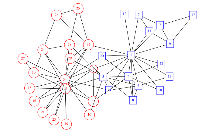
Figure 1: Zachary’s friendship network [17] of the “troubled” karate club consisting of $34$ vertices and $78$ edges. Here open squares and circles are used to denote the supporters, in the ongoing conflict, of the trainer (node $1$) and administrator (node $34$), respectively.

A current mapping, based on Zachary’s tie data, will now be conducted and the results of such an analysis compared against the known structure of the network. Fig. 2(a) shows the $1$-dimensional projection of the network for the slowest decaying ($\alpha=2$) mode. As a guide to the eye, we have here labeled the vertices according to the convention used in Fig. 1, but it should be stressed that this information has not been used during the analysis. Fig. 2(a) shows a striking division of the vertices into two groups corresponding to positive and negative values of $c^{(2)}_{i}$. This division is fully consistent with the original classification made by Zachary. Hence, the slowest decaying diffusive mode $\alpha=2$ of the karate club network can be associated with the trainer–administrator separation. The modularities corresponding to this division are $Q^{(2)}=0.404$ and $Q_{A}^{(2)}=0.371$, where $Q_{A}$ refers to the modularity using the unweighted adjacency matrix, but the same partitioning, for its calculation.

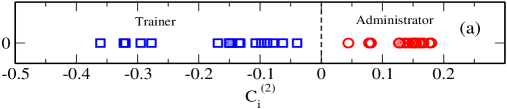
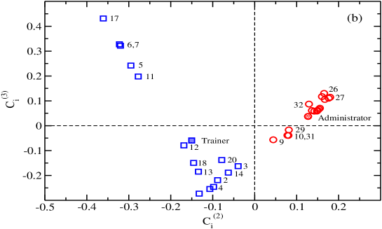
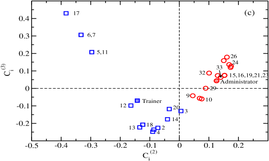
Figure 2: The lowest order current projections of the Zachary network. The (a) $c^{(2)}_{i}$ and (b) $c^{(2)}_{i}c^{(3)}_{i}$ current projections of the weighted network, and (c) the $c^{(2)}_{i}c^{(3)}_{i}$ mapping for the corresponding unweighted network (result taken from Ref. [7]).

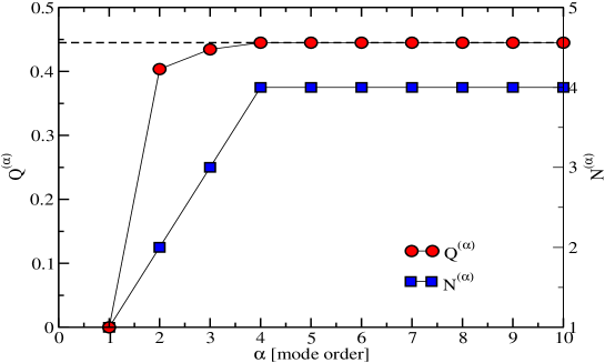
Figure 3: The modularity $Q^{(\alpha)}$ (left axis) and number of communities $N^{(\alpha)}$ (right axis) vs relaxation mode $\alpha$ for the Zachary network of Fig. 1. It is observed that after mode $\alpha=4$ no more communities are identified. The partitioning into four corresponds to a modularity of $Q=0.445$ (weighted network) and $Q_{A}=0.420$ (unweighted network). The optimal value of $Q$ is indicated as a dashed horizontal line in the figure.

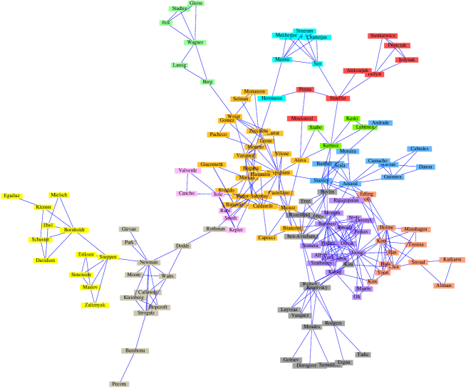
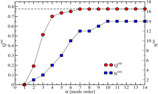
Figure 4: A “network” scientists collaboration network (see Refs. [9, 19] for details). (a) The largest component, consists of $N=145$ vertices, of this network. Figure after Ref. [9], where colors correspond to communities found there. (b) Same as Fig. 3, but for the network of Fig. 4(a). The optimal partitioning is found for $14$ communities characterized by the modularities $Q=0.78$ and $Q_{A}=0.70$.

Fig. 2(b) presents the results of performing a $2$-dimensional current mapping of the network (modes $\alpha=2,3$). The results suggest that the communities associated with the trainer and administrator may be further sub-divided. In particular, the members $\{5,6,7,11,17\}$ are well separated from the rest of the supporters of the trainer with different signs for the $c^{(3)}_{i}$ currents. A close inspection of the network (Fig. 1) reveals that these members are connected to the rest of the network only via the trainer. They may therefore serve as good candidates for forming a trainer sub-community. The supporters of the administrator do also map to $c^{(3)}_{i}$-currents of different signs. However, in this case, the currents are more clustered around $c^{(3)}_{i}=0$ and no striking separation between them exist. It is therefore not clear that this separation can be attributed to a administrator sub-community. This is, indeed, confirmed by investigating the values of the modularity of the possible divisions. Based on the $2$-dimensional current space, a division into three community is optimal ($Q^{(3)}=0.435$); an administrator community, and two communities where one consists of members $\{5,6,7,11,17\}$, while the other one consists of the remaining supporters of the trainer. Insisting on four communities corresponding to the vertices located in each of the quadrants of the $2$-dimensional current plot (Fig. 2(b)), would have given a modularity of $0.423$. This is smaller than $Q^{(3)}$ and this latter partitioning was therefore rejected compared to the chosen one. It is interesting to observe that if one had based the analysis on the unweighted network [7], the results would have been rather similar (Fig. 2(c)), but vertex $3$, for instance, would not have been correctly identified, and there would have been more “degeneracy” among the current values.

Increasing the dimension of the projection space will introduce new potential partitions that may be accepted or rejected. The results of gradually increasing the dimension of the projection space are depicted in Fig. 3. Therefrom it is observed that the optimal partitioning of the network, according to our algorithm, is into $4$ communities that correspond to a modularity of $Q=Q^{(4)}=0.445$ and $Q_{A}=Q_{A}^{(4)}=0.420$. Adding new modes beyond $\alpha=4$ will not improve the partitioning. The members of the last community, not given above, are $\{24,25,26,28,29,32\}$. For the same network, four communities was also reported by Newman and Girvan [9]. However, their communities (for the best partitioning) were put together a little differently resulting in a slightly lower modularity than the one reported here. Donetti and Muñoz [10], on the other hand, identified the same communities as we did, but in addition, they had a single vertex community (vertex 12). In effect, this difference resulted in a slight decrease in the modularity compared to the results reported here. For the karate club network, the partitioning given herein, results in, to the best of our knowledge, the highest modularity values reported for this network.

4.2 Scientific collaboration network

The network under scrutiny in this subsection is a collaboration network of scientists that have published work together. The data set originates from Park and Newman [19] and was later restudied in Ref. [9]. The network was constructed by taking an initial list of “network” scientists (actually those appearing in the reference list of Ref. [5]) and cross-reference those names against the physics e-print archive arxiv.org in search for joint publications. If, at least, one joint work was found, an edge was created between these two scientists. Its weight depended on the number of joint publications as well as the number of co-authors taking part in the joint work. Please consult Ref. [19] for further details regarding this network. The largest component of the resulting network is presented in Fig. 4(a). This component consists of $N=140$ scientists with the present author being among them. This network component was recently analyzed by Newman and Girvan [9] who reported an optimal partitioning (using his method) consist of $13$ communities characterized by a modularity of $Q_{A}=0.72\pm 0.02$.

The findings using the current mapping clustering technique, are summarized in Fig 4(b). It is seen that the optimal number of clusters is found to be $14$. The corresponding modularities were $Q=0.78$ and $Q_{A}=0.70$, comparable to the result reported in Ref.  [9]. We do not here intend to delve into a detailed discussion on the networks community structure. However, it should be add that our findings for the community structure follow mainly the structure reported by Newman and Girvan (and indicated by vertex colors in Fig. 4(a)).

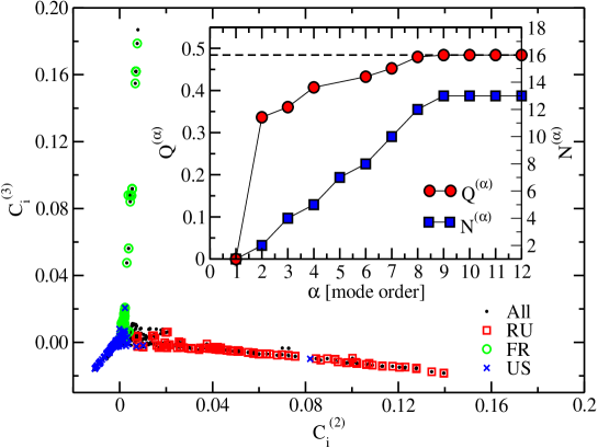
Figure 5: The two-dimensional current mapping of an Autonomous System (AS) network [6, 20]. The symbols refer to the geographical location of the AS: Russia ($\Box$), France ($\bigcirc$), USA ($\times$). The inset shows the modularity and number of communities for the optimal partitioning of the network at a given diffusive mode.

4.3 Autonomous systems

The last example that will be considered herein is a relatively large network where the (about $6\,500$) vertices represent so-called autonomous systems (AS), while the edges corresponds to an entry in the (dynamic) routing table of those devices at the time of observation [20]. These networks are changing with time, and their structures are not known in advance.

Fig. 5 shows the $2$-dimensional current mapping of the networks. The star-like structure indicates that there is a hierarchy of vertices where those located the furthest away from the origin of the current plot are the most peripheral vertices of the network. Furthermore, each hierarchy corresponds roughly to the national division of the autonomous systems network. Fig. 5 shows that the three legs of the star-structure correspond to Russia, the US and France. For the AS-network we identified $13$ communities resulting in a modularity of about one-half.

5 Conclusions

We have considered random walks on weighted networks. This auxiliary network process is used to obtain information on the large scale topological structure of the underlying network. This is done by projecting the nodes of the network onto a low dimensional current space. In this space, vertices that are connected to one another are likely to appear close to each other. This is a consequence of the relaxation towards the stationary state being non-uniform; it is fastest in well connected regions, therefore quickly reaching a quasi-stationary state here, and slow between poorly connected regions. It was found that the weights of the edges of the network may be important to take into consideration in order to reveal the correct underlying topology. Furthermore, this work explicitly demonstrates that the concept of diffusion, or random walks, is a powerful tool that can be applied successfully to problems where no natural connection to diffusion exists.

References

- [1] A. Einstein, Ann. Phys. 17 (1905) 549.
- [2] A. Einstein, Investigations on the Theory of Brownian Movement (Dover, New York, 1956).
- [3] B.D. Hughes, Random Walks and Random Environments, Vol. 1: Random Walks, (Oxford University Press, New York, 1995).
- [4] R. Albert and A.-L. Barabasi, Rev. Mod. Phys. 74 (2002) 47.
- [5] M. Newman, SIAM Rev. 45 (2003) 167.
- [6] K. A. Eriksen, I. Simonsen, S. Maslov, and K. Sneppen, Phys. Rev. Lett. 90 (2003) 148701.
- [7] I. Simonsen, K. A. Eriksen, S. Maslov, and K. Sneppen, Physica A 336, (2003) 167.
- [8] M. Girvan and M. E. J. Newman, Proc. Natl. Acad. Sci. USA 99 (2002) 7821.
- [9] M. E. J. Newman, and M. Girvan, Phys. Rev. E 69 (2004) 026113.
- [10] L. Donetti and M. A. Muñoz, J. Stat. Mech.: Theor. Exp. (2004) P10012.
- [11] E. Almaas P.L. Krapivsky and S. Redner, Statistics of Weighted Networks, to appear Phys. Rev. E.
- [12] M. E. J. Newman, Phys. Rev. E 70 (2004) 056131.
- [13] C.D. Meyer, Matrix analysis and applied linear algebra, SIAM, 2000.
- [14] A.K. Jain and R.C. Dubes, Algorithms for clustering of data (Englewood Cliffs. New Jersey, Prentice-Hall, 1988).
- [15] H. Spaeth, Cluster Analysis Algorithms for Data Reduction and Classification of Objects Ellis Horwood 1980).
- [16] J. Hartigan, Clustering algorithms (New York, Wiley, 1975).
- [17] W. W. Zachary, J. Anthropol. Res. 33 (1977) 452473.
-
[18]
The Zachary network can be downloaded from :
http://vlado.fmf.uni-lj.si/pub/networks/data/UciNet/zachary.dat. - [19] J. Park and M.E.J. Newman, Phys. Rev. E 68 (2003) 026112.
- [20] The data set can be obtained from http://moat.nlanr.net/AS/.