On the form of growing strings

Abstract

Patterns and forms adopted by Nature, such as the shape of living cells, the geometry of shells and the branched structure of plants, are often the result of simple dynamical paradigms[1]. Here we show that a growing self-interacting string attached to a tracking origin, modeled to resemble nascent polypeptides in vivo, develops helical structures which are more pronounced at the growing end. We also show that the dynamic growth ensemble shares several features of an equilibrium ensemble in which the growing end of the polymer is under an effective stretching force. A statistical analysis of native states of proteins shows that the signature of this non-equilibrium phenomenon has been fixed by evolution at the C-terminus, the growing end of a nascent protein. These findings suggest that a generic non-equilibrium growth process might have provided an additional evolutionary advantage for nascent proteins by favoring the preferential selection of helical structures.

82.35.Lr,82.30.Fk,36.20.Ey,87.15-v

Non-equilibrium and pattern formation studies have a profound influence on in vivo biology [1]. The dynamical evolution of the branched actin cytoskeletal network which pushes a cell forward  [2], the spatial self-organisation of genome during DNA replication and transcription [3], and the synthesis of a nascent protein within a ribosome [4, 5] are just a few examples in which non-equilibrium physics becomes relevant to cell biology. In order to make contact with these phenomena occurring within the cell, in vitro experiments on polymer dynamics employing single molecule techniques are nowadays routinely made. These are amenable to a detailed analysis and to comparison with theory. Examples include DNA packaging in the $\Phi$29 bacteriophage [6], DNA or polymer translocation through a membrane pore [7], the rheology of a single molecule of DNA under shear or elongational flow [8] and the elasticity of F-actin networks [9]. These experiments draw on the ability to micro-manipulate biopolymers with high accuracy, and even at the single molecule level [10], employing atomic force microscopes, soft micro-needles, laser tweezers and other micro or nanoscopic devices.

Despite their importance, studies in polymer dynamics out of or far from equilibrium pose serious theoretical challenges and have not been systematically investigated so far. Here we report evidence for the existence of a non-equilibrium pattern selection favoring the formation of helices during the growth of a self-interacting polymer from a tracking origin, mimicking the situation occurring when nascent proteins are produced[4, 5]. We show by numerical simulations that the dynamic ensemble we consider shares many features of an equilibrium ensemble in which the newly grown polymer segment is under a stretching force, and we discuss where the ”dynamic” force comes from in our simulations. Finally, by an analysis of protein structures from the Protein-Data-Bank, we observe that the dynamic preference for helices we pinpoint has been fixed by evolution in the folded structure of proteins and we speculate why it might be so.

We modelled the growth of a flexible self-interacting polymer attached to a moving, or tracking, origin by means of molecular dynamics [11]. We work in the reference frame of the tracking origin. The polymer is modelled by a chain of $N$ beads, at positions $\left\{\vec{r}_{i}\right\}_{i=1,\ldots,N}$ in the three-dimensional space. The growth process starts from a conformation which contains a single bead placed at the origin of the reference frame. After a repeated constant time interval, a new bead is added at the position of the growing end and the rest of the chain is translated upward (always in the positive $z$-direction) by one link. The polymeric beads are tethered by a harmonic potential between any two consecutive residues, given by

$$V(r)=k(r-b)^{2}\;,$$ (1)

with $r$ their mutual distance, $b$ the equilibrium length of a link and $k$ the spring constant. Non-consecutive residues interact via a 6-12 Lennard-Jones (LJ) potential mimicking a poor solvent,

$$V_{LJ}(r)=4\epsilon\left(\left(\frac{\sigma}{r}\right)^{12}-\left(\frac{\sigma}{r}\right)^{6}\right),$$ (2)

where $\sigma$ and $\epsilon$, determining the range and strength of the LJ potential, also define the length and energy scales in our model. The unit of time is $\tau\equiv\sqrt{m\sigma^{2}/\epsilon}$ where $m$ is the mass, identical for every residue. We have chosen $b=0.78\sigma$, so that the ratio $\sigma/b$ is close to that of a polypeptide chain, and $k=2500\epsilon/\sigma^{2}$. Coupling of the chain with the surrounding solution is given by a damping term and the Langevin noise that compensates the drag force in order to maintain constant temperature, $T$. The equations of motion for each bead are

$$m\ddot{\vec{r}_{i}}=-\gamma\dot{\vec{r}_{i}}+{\vec{F}_{c}}+{\vec{\Gamma}},$$ (3)

where ${\vec{F}_{c}}$ is the net force due to molecular potentials (1) and (2), $\gamma$ is the friction constant and ${\vec{\Gamma}}$ is a Gaussian noise with dispersion $\sqrt{2\gamma k_{B}T}$. We have chosen $\gamma=10m/\tau$ which is above the overdamping limit [12]. The equations of motion are integrated by means of the fifth-order Gear predictor-corrector algorithm [13] with a time step of 0.005$\tau$. The simulations are carried out at near zero temperature, $T=0.02\epsilon/k_{B}$, in order to provide a highly stabilizing condition. The growth rate, $r_{growth}$, is measured as number of beads grown per unit time.

The steady state regime of the configurations resulting from the growth simulations is characterised by a dynamic coexistence of polymer segments - or blobs - which are associated with a various degree of equilibration. Due to the attractive self-interactions, mimicking van der Waals forces in polypeptides, the patterns near the growing end depend crucially on the ratio between the growth and the relaxation rates. Representative configurations obtained by molecular dynamics simulations of the growth process are shown in Fig. 1. If the growth rate, $r_{growth}$, is small compared to the relaxation rate, $\tau_{\rm relax}^{-1}$, ($\tau_{\rm relax}$ being the characteristic time needed for the system to equilibrate) the string has the time to equilibrate and a rather compact and structureless conformation is obtained (Fig. 1d). The most interesting situation occurs when the two rates are comparable, $r_{growth}\tau_{relax}\sim 1$ (Fig. 1a–c). Near the growing end the polymer self-organises into a helix or a zig-zag structure, with its axis parallel to the growth direction. As string segments age and get farther away from the growing end, they can organise themselves into alternative shapes corresponding to different free energy minima. For large growing rates, $r_{\rm growth}\tau_{\rm relax}\gg 1$ the polymer is stretched as if under the action of a pulling force. We consider two cases: (i) the growing end is kept fixed at the origin of the reference frame (this more closely mimics the situation of a nascent peptide inside the ribosomal exit tunnel), and (ii) the growing end is free. While in both cases the results are qualitatively similar, in the former case (shown in Fig. 1) the helix is longer and it is formed over a wider range of $r_{growth}$. In both cases, the ranges of stability of the helix and the zig-zag structure are enhanced as T decreases, i.e. they can form at slower and wider ranges of the growth rates. This is mainly due to the enhancement of the free energy barrier to be crossed to enter the globule phase which effectively raises $\tau_{relax}$.

The phenomenon of pattern selection that we observe is mainly caused by the lack of time for the growing portion of the chain to fold into a globule, so that only local contacts along the string can be established. However, a priori, other different periodic or less regular structures with local contacts are possible during the growth and thus the selection of a particular helix is rather a surprise. The pitch to radius ratio of the helix depends on the details of the self-interaction potential used for the string (in our case the ratio between $\sigma$ and $b$). In Fig. 1c, instead, the aging end is becoming less ordered and more compact than the helix at the growing end. It should be noted that the relaxation time of a polymer is expected to have a power law dependence on the number of residues $N$, $\tau_{\rm relax}\sim\tau_{0}N^{\alpha}$, where $\alpha=2$ if the dynamics is Brownian and $\alpha\approx 1.7$ if long range hydrodynamic interactions dominate the dynamics [14]. Thus, given any growth rate, if we wait long enough, the number of grown beads increases and $r_{\rm growth}\tau_{\rm relax}$ will eventually become comparable to 1.

It is instructive to compare the conformations observed during the growth of a polymer (Fig. 1) with those resulting from simulated pulling experiments (Fig. 2). We consider the same inter-bead potential (1) and (2) used for the growth simulations. We considered two different ensembles in which a simulated pulling experiment can be performed: (a) a ’fixed force’ mode in which the string is subject to a constant force and (b) a ’fixed stretch’ mode in which one end of the string is fixed and the other one is moved. with a very low velocity so that the string is always found in a near equilibrium condition. In case (a) the controlled parameter is the magnitude of the pulling force, $f$, while in case (b) it is the stretching velocity $v$. Fig. 2 shows the set-up and the sketched ‘phase diagrams’ with representative ground state structures obtained with simulations of string pulling in modes (a) and (b). These ‘phase diagrams’ could be tested with single molecule stretching experiments. This suggests that the dynamic growth ensemble shares the qualitative features of a fixed force ensemble near the newly grown portion of the polymer [15].

In our growth simulations, this effective “stretching” at the growing end is due both to the drag exerted by the more globular and equilibrated “older” sections of the string onto the newly grown ones, and to the inability of the newly grown segment to equilibrate before a new segment of the string is grown. The growth mechanism that we consider resembles the one occurring in vivo when a nascent protein (the ”self-attracting string”) is synthesised in the ribosome (the ”origin”, which is tracking along the mRNA). The results that we presented show that non-equilibrium effects lead to specific pattern selection already in a generic self-interacting polymer. This kinetic effect does not compete with other well-known thermodynamic factors which stabilizes $\alpha$-helices in proteins, such as hydrogen bonds[16] and steric interactions[17]. Furthermore, stereochemical considerations suggest that the nascent protein can exit from the tunnel in an $\alpha$ helical conformation [18]. The dynamic selection of helices may couple to the chemistry to yield a robust mechanism for helices formation during the very early stages of protein folding. Still, what may the dynamic ”stretching” come from during in vivo protein translation ? The ribosomal translation rate is about 45 or so nucleotides per second [18]. Viscous drags would then be $\ll$ 1 pN for objects of the size of proteins (the viscosity of cytosol for proteins is $\sim 1-10$ cP [19]) so they are unlikely to be responsible for any co-translational stretching. On the other hand, protein folding times are typically smaller than even the total growth time. In particular, $\beta$ sheets [20] fold on the millisecond timescale [12], while the inverse growth rate is $\sim$ $0.1$ s (see above). In narrow channel, however, such as the ribosomal exit tunnel (as tight as 2 nm in diameter, and 10 nm long, see [4]), equilibration times increase significantly [21], and $\beta$ formation may become sterically hindered, so that the ratio of these two numbers may match that seen in our simulations when helices are formed. Furthermore, once a helix is formed during the very early stages of a newly grown segment, disrupting it will involve going over a free energy barrier $\Delta F$ so that the formation of more equilibrated structures will require much longer (exponential in $\Delta F/T$) than in an in vitro experiment, where the folding has not been a priori “biased” towards any local minimum.

Finally, we have analysed the protein structures in the Protein Data Bank (PDB) [22] in order to verify whether the non-equilibrium phenomenon predicted here has left a signature even in the native state of proteins, which is usually assumed to be determined by equilibrium considerations alone. We considered protein structures determined by X-ray diffraction and with less than 30% sequence identity, in order to remove homologous structures [23]. Furthermore, we removed proteins that are significantly disordered at their termini, i.e. when more than five residues from either terminus are unstructured. The propensities of forming $\alpha$-helix and $\beta$-strand as functions of residue position away from the termini were computed based on the secondary structure assignment recorded in the PDB file (we have discarded structures for which such an assignment is not present). In order to better test our prediction we divided our final set of about 600 proteins into two groups with their relative contact order (CO) [24] greater than and smaller than 0.15. The aim of doing this division is to classify proteins into slow and fast folding, respectively, at least in an approximate way [24]. For the former group of proteins the effect we expect should be less pronounced and indeed we do not see any clear preference from either termini (data not shown). On the contrary the selection effect is clearly visible in the second group of proteins characterized by small CO (Fig. 3a). For this group of proteins the helical propensity has a peak in the vicinity of both termini but the peak closest to the C-terminus is significantly higher than the one associated with the N-terminus. The $\beta$ strand propensity, instead, follows an inverse tendency. Therefore, the signature of the preferential formation of helices at the C-terminal end of a protein, which results as a consequence of a non-equilibrium effect in nascent polypeptides, has been fixed by evolution. These results are also compatible with the observation that in many proteins translation and folding occur simultaneously during synthesis [18]. To further support the prediction that non-equilibrium effects are key factors leading to the helical preference at the C-terminus we have found that the concentrations of the various types of amino acids are similar at both the N- and C-termini 20-residue fragments, within the error bars provided by the statistics (Fig. 3b). Fig. 3a also shows that the helical propensity as a function of the distance from the C terminus displays oscillations, which may be either simply due to stochasticity or to the typical length of a helical segment in the folded state of proteins.

In conclusion, we suggest that proteins might have taken advantage of the dynamical principle for preferential selection of helices, described here, to select a polypeptide growth mechanism that can bias the backbone configuration of a nascent protein into a state rich in $\alpha$ helices. Our conjecture is supported by the existence of a higher propensity of forming helices near the C-terminus of relatively fast folding proteins. Furthermore this scenario is consistent with at least two lessons we know. First, the reduction of regions rich in $\beta$ sheets would render protein misfolding and aggregation into amyloid like structures less likely [25]. Second, this particular folding mechanism would minimize the role of non local contacts, thus rendering folding faster. It seems appealing that the cell translation machinery has evolved in such a way as to find an optimal compromise between the minimisation of errors and the maximisation of speed in the translation from RNA to nascent proteins.

We have learnt that A. Laio and C. Micheletti have independently observed the higher propensity of the C-terminus to form helices. This work was supported by COFIN MURST 2003, EPSRC and the Natural Science Council of Vietnam (grant no. 410704) . We are greatful to the referees for their very helpful comments.

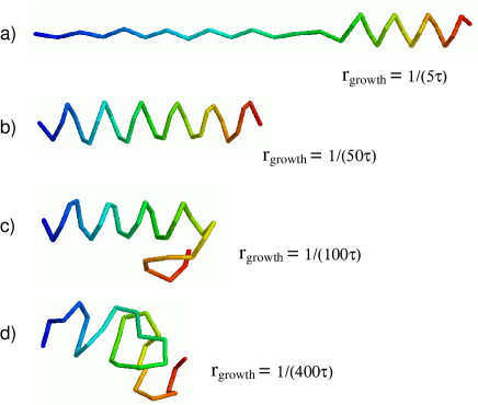
FIG. 1.: Conformations of a growing chain for various $r_{growth}$ as indicated ($\tau$ is defined in the text). The polypeptide chains shown are all of 30 residues. The chain is grown from the left end and the growing end is kept fixed. The growth rates decrease from top to bottom. In a rather wide range of intermediate growth rates (b and c) an ordered helix is formed at the growing end and another one, more distorted and equilibrated, appears at the other end. $\tau_{relax}$, at the growth temperature, is estimated to be $\sim 80$ $\tau$.

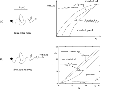
FIG. 2.: Left, schematic representation of two single molecule stretching experiments that we discussed: (a) fixed force mode, (b) fixed stretch mode. Right, sketch of the phase diagram at $T=0$. The minima were found with molecular dynamics and Monte-Carlo simulations at low $T$ and varying force (in (a)) and end-to end distance (in (b)). In (b), the velocity is small so that the string is always in quasi-equilibrium. Most of the stable states in Fig. 2b are characterised by a coexistence of two states found in Fig. 2a. $N$ refers to the length of the polymer.

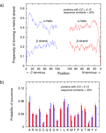
FIG. 3.: (a) Propensity of forming helices and strands as function of residue position away from C-terminus (blue) and N-terminus (red). The data are computed based on a PDB set of 291 non-disordered protein structures with CO smaller than 0.15 and with the secondary structures assignment given in the PDB files. To determine a propensity at a given position we only took proteins with length greater than double the position number, in order to avoid interference from the opposite end. (b) The amino acid concentrations in 20-residue fragments associated with the N- (red) and C-terminus (blue) computed from the same set of proteins used in the top figure (amino acids are labeled with the one letter code).

REFERENCES

- [1] D. Thompson, On Growth and Form (1917).
- [2] T. P. Stossel, Science 260, 1086 (1993).
- [3] B. Alberts et al., Molecular Biology of the Cell, Garland, (1994).
- [4] R. Berisio et al., Nat. Struct. Biol. 10, 366 (2003).
- [5] H. Do et al., Cell 85, 369 (1996).
- [6] D. E. Smith et al.,Nature 413, 748-752 (2001).
- [7] A. Meller, L. Nivon, D. Branton, Phys. Rev. Lett. 86, 3435 (2001).
- [8] D. E. Smith, H. P. Babcock, S. Chu, Science 283, 1724 (1999).
- [9] M. L. Gardel et al.,Science 304 1301 (2004).
- [10] C. Bustamante, Z. Bryant, S. B. Smith, Nature 421, 423 (2003).
- [11] T. X. Hoang, M. Cieplak, J. Chem. Phys. 112, 6851 (2000).
- [12] D. K. Klimov, D. Thirumalai, Phys. Rev. Lett. 79, 317 (1997).
- [13] W. C. Gear, Numerical initial value problems in ordinary differential equations, New York: Prentice-Hall, Inc. (1971).
- [14] M. Doi, S. F. Edwards, The theory of polymer dynamics, Clarendon, Oxford (1986).
- [15] It is also interesting to parallel the dynamic coexistence of string segments we found in the growth model with the static coexistence of blobs upon stretching a polymer in a poor solvent (see Fig. 2b). In this context, the static blob coexistence is a consequence of the Rayleigh instability [B. J. Haupt, T. J. Senden, E. M. Sevick, Langmuir 18, 2174 (2002)].
- [16] L. Pauling, R. B. Corey, H. R. Branson, Proc. Natl. Acad. Sci. USA 37, 205 (1951).
- [17] G. N. Ramachandran, V. Sasisekharan, Adv. Protein Chem. 23, 283 (1968).
- [18] A. N. Fedorov, T. Baldwin, J. Biol. Chem. 272, 32715 (1997).
- [19] K. Luby-Phelps, Int. Rev. Cytol. 192, 189.
- [20] We should compare the growth rate with the rate of formation of non-helical structures (among which structures are the fastest to fold), as the dynamic effect already favors helix formation (which occurs in solution in microseconds).
- [21] R. M. Jendrejack et al., Phys. Rev. Lett. 91, 038102 (2003).
- [22] H. M. Berman et al.,Nucleic Acids Research 28, 235-242 (2000).
- [23] C. Sander, R. Schneider, Proteins 9, 56 (1991).
- [24] K. W. Plaxco et al., Biochemistry 39, 11177 (2000).
- [25] C. M. Dobson, Nature 426, 884 (2003).