Heat conduction in one-dimensional lattice dynamical systems
far from equilibrium

Abstract

We study heat conduction in one dimensional lattice dynamical systems far from equilibrium. The Fermi-Pasta-Ulam model and the $\phi^{4}$ model are numerically compared to elucidate differences between momentum-conserving and nonconserving systems. As a results, it is found that the heat flux in the $\phi^{4}$ model does not increase monotonically as the temperature differences at the ends of the lattice is increased, while it does in the FPU chain.

Currently, heat conduction in one-dimensional systems is getting more and more attention in nanoscale physics. Murayama studied heat conduction in the single walled carbon nanotube and found that the thermal conductivity behaves like one-dimensional systems. [1] Namely, the thermal conductivity a nanotube with a small diameter did not converge to a finite value with increase in tube length, but obeyed a power law relation as is observed in the one-dimensional systems. Similar behavior was observed in the nanoscale world by several authers[2, 3].

In macroscopic systems, heat conduction obeys the Fourier’s law

$$J=-\kappa\nabla T,$$ (1)

where $J$ and $\nabla T$ denote the heat flux and the temperature gradient. Recent studies in one-dimensinal systems have clarified that size-dependence of the thermal conductivity $\kappa$ is different between momentum-conserving and nonconserving systems. For example, the thermal conductivity diverges as $\kappa\sim N^{0.37}$ in the FPU chain, where the momentum is a conserved quantity[4]. On the other hand, it converges in the limit of large system size in the $\phi^{4}$ model, where momentum is not conserved due to the existence of on-site potentials. This principle is also applied to the diatomic Toda chain[11], the Frenkel-Kontrova model[6, 7], the ding-a-ling model[8], the ding-dong model[9], and many others, though the integrable systems like the harmonic chain or the Toda lattice show another behavior $\kappa\sim N$ and there are some exceptions to the principle[12, 14]. Now, this behavior is understood as an effect of long-time tail in the autocorrelation function of the total heat flux[13].

On the other hand, in nanoscale devices, the temperature gradient need not be small and heat conduction is not necessarily described by the Fouries’s law. Thus, heat conduction beyond the linear-response regime can be observed in nanoscale physics. Accordingly, we study in this paper properties of heat conduction far from equilibrium, and particularly look into differences between momentum-conserving and nonconserving models.

We consider one-dimensional systems with Hamiltonian of the type

$$H=\sum_{i=1}^{N}\biggl{[}\frac{p_{i}^{2}}{2}+U(q_{i})\biggr{]}+\sum_{i=0}^{N}V(q_{i+1}-q_{i}),$$ (2)

where $q_{i}$ and $p_{i}$ denote the displacement and the momentum of the $i$th particle, $U(q_{i})$ the on-site potential and $V(q_{i+1}-q_{i})$ the interaction potential between nearest-neighbor particles. We use the fixed boundary condition, whch is represented by putting $q_{0}=q_{N+1}=0$ in Eq. (2). We consider the following two models: (i) the FPU model is described by $V(q)=\frac{1}{2}q^{2}+\frac{1}{4}q^{4}$ and $U(q)=0$ and (ii) the $\phi^{4}$ model is decribed by $V(q)=\frac{1}{2}q^{2}$ and $U(q)=\frac{1}{2}q^{2}+\frac{1}{4}q^{4}$.

Moreover, two heat reservoirs are attached to the system, that is, particle $1$ is in contact with a heat reservoir at temperature $T_{L}$ and particle $N$ is in contact with another heat reservoir at temperature $T_{R}$. In the present study, we use three kinds of heat reservoirs, the Langevin thermostats, the Nose-Hoover thermostats, and the thermal wall. In the Langevin thermostats, random forces and dissipation terms are introduced into the equations of motion. Namely, the equations of motion of particles $1$ and $N$ are

$$\dot{p}_{1}=-U^{\prime}(q_{1})+V^{\prime}(q_{2}-q_{1})-V^{\prime}(q_{1})-\gamma_{L}p_{1}+\xi_{L}(t)$$

$$\dot{p}_{N}=-U^{\prime}(q_{N})+V^{\prime}(-q_{N})-V^{\prime}(q_{N}-q_{N-1})-\gamma_{R}p_{N}+\xi_{R}(t),$$

where $\gamma_{\alpha}$ denotes the coupling strength between the particle and the heat bath and $\xi_{L}(t)$ and $\xi_{R}(t)$ are the Gaussian white noise with zero mean and variance

$$\langle\xi_{\alpha}(t)\xi_{\beta}(t^{\prime})\rangle=2\gamma_{\alpha}T_{\alpha}\delta_{\alpha\beta}\delta(t-t^{\prime}),\quad(\alpha,\beta=R,L).$$ (3)

In the case of Nose-Hoover thermostats, deterministic forces play the role of heat reservoir. Namely, the equations of motion for particles 1 and $N$ are modified as

$$\dot{p}_{1}=-U^{\prime}(q_{1})+V^{\prime}(q_{2}-q_{1})-V^{\prime}(q_{1})-\xi_{L}p_{1},\quad\dot{\xi_{L}}=\frac{1}{\Theta}\biggl{(}\frac{p_{1}^{2}}{T_{L}}-1\biggr{)},$$

$$\dot{p}_{N}=-U^{\prime}(q_{N})+V^{\prime}(-q_{N})-V^{\prime}(q_{N}-q_{N-1})-\xi_{R}p_{N},\quad\dot{\xi_{R}}=\frac{1}{\Theta}\biggl{(}\frac{p_{N}^{2}}{T_{R}}-1\biggr{)},$$

where $\Theta$ is the thermostat response time. In the thermal wall, if a particle hits the wall, it is reflected with a momentum randomly chosen according to the distribution

$$f(p)=\frac{|p|}{T}\exp\biggl{(}-\frac{p^{2}}{2T}\biggr{)},$$ (4)

where $T$ is the temperature of the wall.

In our numerical simulations, the 4th-order Runge-Kutta and the 6th-order symplectic integrator were used in the Langevin and the Nose-Hoover cases. In the cases of the thermal walls, the 4th-order Symplectic Integrator was employed. All the simulations were done with a time step $\Delta t=0.01$ and the parameters are chosen as $\gamma_{L}=\gamma_{R}=0.5$ and $\Theta=0.1$. The temperature of particle $i$ is defined as kinetic temperature $T_{i}=\langle p_{i}^{2}\rangle$ and local heat flux through particle $i$ is given by

$$j_{i}=\frac{1}{2}(p_{i+1}+p_{i})F(q_{i+1}-q_{i}).$$ (5)

Both the quantities were obtained with averaging over $10^{10}$ time steps in the $\phi^{4}$ model and $10^{9}$ time steps in the FPU model after a nonequilibrium steady state was reached.

(a)	(b)

Figure 1: Temperature profile for the FPU model (a) and the $\phi^{4}$ model (b) with system size N=32 and the Langevein thermostats, the Nose-Hoover thermostats and the thermal walls at $T_{L}=2.0$ and $T_{R}=1.0$.

Figure 1 shows the temperature profile for the $\phi^{4}$ model and the FPU model near equilibrium steady states. We see that smooth temperature profile is formed except for boundaries, where temperature gaps exist.

(a)	(b)

Figure 2: Temperature profile for the FPU model (a) and the $\phi^{4}$ model (b) with system size N=32 and the Langevein thermostats, the Nose-Hoover thermostats and the thermal walls at $T_{L}=40.0$ and $T_{R}=1.0$.

When the temperature difference between the two heat reservoirs is larger, the system is beyond the linear response regime and then Fourier’s law does not hold. Figure 2 shows the temperature profile in the $\phi^{4}$ model and the FPU model, respectively. In the FPU model, the temperature profile is qualitatively similar to the near-equilibrium case. Only difference is that the gaps between the heat reservoirs and particle $1$ or $N$ become larger than the near-equilibrium case. On the other hand, in the $\phi^{4}$ model, the temperature profile is drastically transformed. Namely, local temperatures are largely shifted to low values in the bulk region and changes are notable only near the end at the higher temperature.

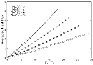
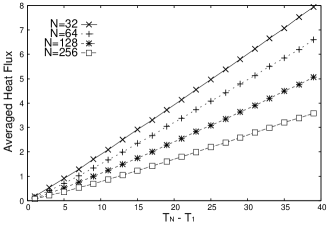
(a)	(b)
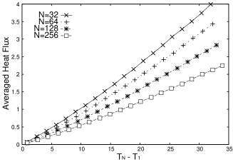
(c)

Figure 3: Averaged heat flux and temperature difference at both ends for the FPU model with the Langevein thermostats (a), the Nose-Hoover thermostats (b) and the thermal walls (c).

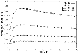
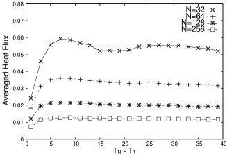
(a)	(b)
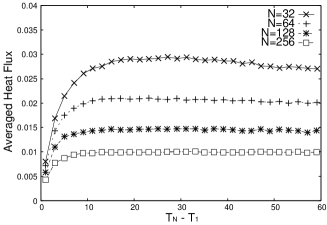
(c)

Figure 4: Averaged heat flux and temperature difference at both ends for the $\phi^{4}$ model with the Langevein thermostats (a), the Nose-Hoover thermostats (b) and the thermal walls (c).

Heat flux also shows peculiar behavior. Figures 3 and 4 show the mean heat flux as a function of the temperature difference $T_{N}-T_{1}$.

$$j=\frac{1}{N}\sum_{i=1}^{N}j_{i},$$ (6)

where $j_{i}$ is the local heat flux at the $i$th site defined by

$$j_{i}=\frac{1}{2}(p_{i+1}+p_{i})F(q_{i+1}-q_{i}),$$ (7)

where $F(x)=-\frac{d}{dx}V(x)$. It is observed that as the temperature difference increases, the averaged heat flux increases monotonically in the FPU model. In the $\phi^{4}$ model, however, the averaged heat flux saturates at some value of temperature difference and does not increase further. Similar results are obtained irrespective of the types of heat reservoirs. Therefore, these differences are caused only by the characteristic of the lattice dynamical systems.

Moreover, we compute the harmonic interaction potential with and without harmonic on-site potential cases. In these cases, we confirmed that the averaged heat flux increases monotonically. Thus, the peculiar behavior of the $\phi^{4}$ model should be attributed to combination of nonintegrability and lack of momentum conservation. Extensive study to clarify the origin of our findings is planned for the future. Our results may provide a guideline for designing nanoscale devices.

We have studied the heat conduction far from equilibrium in non equilibrium steady states in the FPU and $\phi^{4}$ chains. As a results, we have found the new interesting phenomenon of the heat conduction. In the FPU model, heat flux increases monotonically as temperature difference between particles $1$ and $N$. However, in the $\phi^{4}$ model, heat flux does not increase monotonically. This property does not depend on the heat reservoirs.

AU thanks H. Nishimori, H. Hayakawa, M. M. Sano for valuable discussions and helpful comments. This work is supported by the Grant-in-Aid for the 21st Century COE ”Center for Diversity and Universality in Physics” from the Ministry of Education, Culture, Sports, Science and Technology (MEXT) of Japan. The numerical computation in this work was carried out at Library & Science Information Center, Osaka Prefecture University.

References

- [1] S. Murayama: Physica B 323 (2002) 193.
- [2] Z. Yao, J. Wang, B. Li, and G. Liu: cond-mat/0402616.
- [3] G. Zhang and B. Li: cond-mat/0501194.
- [4] S. Lepri, R. Livi, and A. Politi: Phys. Rev. Lett. 78 (1997) 1896.
- [5] Z. Rieder, J. L. Lewobitz, and E. Lieb: J. Math. Phys. 8 (1967) 1073.
- [6] B. Hu, B. Li, and H. Zhao: Phys. Rev. E 57 (1998) 2992.
- [7] B. Hu, B. Li, and H.Zhao: Phys. Rev. E 61 (2001) 3828.
- [8] D. J. R. Mimnagh and L. E. Ballentine: Phys. Rev. E 56 (1997) 5332.
- [9] M. Sano and K. Kitahara: Phys. Rev. E 64 (2001) 056111.
- [10] S. Lepri, R. Livi, and A. Politi: Europhys. Lett. 43 (1998) 271.
- [11] T. Hatano: Phys. Rev. E 59 (1999) 1063.
- [12] C. Giardiná, R. Livi, A. Politi, and M. Vassali: Phys. Rev. Lett. 84 (2000) 2144; O. V. Gendelman and A. V. Savin, Phys. Rev. Lett. 84 (2000) 2381.
- [13] S. Lepri, R. Livi, and A. Politi: Phys. Rep. 377 (2003) 1.
- [14] C. Giardina and J. Kurchan: J. Stat. Mech. (2005) P05009.
- [15] S. Nose: Prog. Theor. Phys. Suppl. 103 (1991) 1.