Ferroelectricity in Incommensurate Magnets

Abstract

We review the phenomenology of coupled magnetic and electric order parameters for systems in which ferroelectric and incommensurate magnetic order occur simultaneously. We discuss the role that such materials might play in fabricating novel magnetoelectric devices. Then we briefly review the mean-field description of ferroelectricity and modulated magnetic ordering as a preliminary to analyzing the symmetry of the interaction between the spontaneous polarization and the order parameters describing long-range modulated magnetic ordering. As illustration we show how this formulation provides a phenomenological explanation for the observed phase transitions in Ni₃V₂O₈ and TbMnO₃ in which ferroelectric and magnetic order parameters simultaneously become nonzero at a single phase transition. In addition, this approach explains the fact that the spontaneous polarization only appears along a specific crystallographic direction. We analyze the symmetry of the strain dependence of the exchange tensor and show that it is consistent with the macroscopic symmetry analysis. We conclude with a brief discussion of how our approach might be relevant in understanding other systems with coupled magnetic and ferroelectric order, and more importantly, how these principles relate to the search for materials with larger magnetoelectric couplings at room temperature.

I Introduction

The interactions between long-range magnetic order and long-range ferroelectric order have been studied in depth since the first experimental confirmation of the magnetoelectric effect in the late 1950s.DZYALOSHINSKII ; ASTROV ; RADO We note the existence of several reviewsREV1 ; REV2 ; REV3 and monographsBIRSS which give a general overview of the subject.

Of particular interest for this review are those materials which exhibit a combined magnetic and ferroelectric transition. Perhaps the best known of these is Ni-I boracite (Ni₃B₇O₁₃I) which shows coupled ferromagnetic, ferroelectric, and ferroelastric properties at a single phase transition at $T=61.5$ K.ascher ; toledano The multiferroic behavior in this boracite arises from the fact that the magnetic transition is connected to a structural distortion, which in turn allows the development of ferroelectric order.toledano This transition can be understood in terms of a phenomenological Landau theory which couples the ferromagnetic, ferroelectric, and ferroelastic order parameters to a primary antiferromagnetic order parameter.toledano The strong coupling between magnetic and ferroelectric order parameters in systems having a simultaneous phase transition is demonstrated by the observation that in Ni₃B₇O₁₃I it is possible to reverse the direction of the spontaneous polarization by applying an external magnetic field perpendicular to the direction of magnetization.ascher

Cr₂BeO₄ also develops magnetic and ferroelectric order at a single phase transition.newnham Below T=28 K, Cr₂BeO₄ orders antiferromagnetically into a state with spiral spin structure, and this antiferromagnetic state shows an extremely small spontaneous polarization (approximately one million times smaller than that of BaTiO₃). The coupling between magnetic and ferroelectric order is expressed by a model proposing a mechanism in which the electric polarization is induced solely by the antiferromagnetic order.stefanovskii A similar model for magnetically-induced ferroelectric order will be discussed in detail in the following sections.

While the magnetic and ferroelectric transition temperatures for BaMnF₄ are widely separated, this system is useful in illustrating the importance of symmetry considerations in determining magnetoelectric properties. Pyroelectric BaMnF₄ orders antiferromagnetically when cooled below $T=26$ K, and there is a dielectric anomaly at this magnetic transition temperature.samara This decrease in dielectric constant below $T_{N}$ varies like the square of the sublattice magnetization, and clearly indicates a coupling between the magnetic and ferroelectric properties of the sample. This interaction between magnetic and ferroelectric order is attributed to a magnetoelectric coupling which causes a polarization induced spin canting.foxA Substituting 1%Co for Mn changes the magnetic symmetry group of the compound to one which precludes this magnetoelectric coupling,foxB and in turn eliminates the dielectric anomaly at the magnetic ordering temperature. As this system illustrates, in order to understand magnetoelectric couplings in multiferroic systems it is crucial to have complete information about the magnetic and structural symmetries of the system.

Until quite recently, the theoretical and experimental studies have focussed on ferroelectricity in systems with simple ferromagnetic or antiferromagnetic orderfoxB ; toledano (with studies on Cr₂BeO₄ being the notable exception). These systems are tractable from a theoretical standpoint, and allow a comparison to be made between experimental results and straightforward models based on magnetic space groups. However, limiting the scope of investigation to systems with ferromagnetic or antiferromagnetic order neglects a large class of materials which have more complex magnetic structures. Here we will not consider systems (several of which are listed in Table I of Ref. REV1, ) which are ferroelectric at high temperature and then have a lower temperature phase transition at which magnetic ordering takes place.LRO Instead, in this brief review article we will focus on the more recent studies in which ferroelectricity appears simultaneously (in a single combined phase transition) with long-range sinusoidally modulated magnetic order,KIM ; HUR which we will refer to generically as “incommensurate”INCOM magnetic order. Accordingly, we will briefly summarize the experimental situation for the systems TbMnO₃ (TMO)HUR ; TMO and Ni₃V₂O₈ (NVO).PRL ; RAPID ; NVO1 Then we will describe in detail the symmetry analysis developed in Refs. RAPID, , NVO1, , and NVO2, to understand the phenomenology of these systems. We believe that this theoretical approach is simple enough that it can easily be applied to the ever increasing number of systems like NVO or TMO in which ferroelectricity is induced by incommensurate magnetic long-range order.

Figure 1: Adapted from Ref. RAPID, . Spontaneous (i. e. in zero applied electric field) polarization ${\bf P}$ versus applied uniform magnetic field ${\bf H}$ applied along different crystallographic directions at selected temperatures for NVO. The arrows indicate the directions of increasing and decreasing magnetic field.

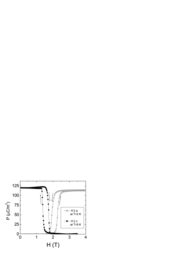
To illustrate this phenomenon, we show, in Fig. 1 some intriguing data from Ref. RAPID, showing that the spontaneous polarization P depends strongly on the applied magnetic field H. At first glance this data seems to have no obvious explanation. However, when viewed in combination with the magnetic phase diagram (see Fig. 6, below) we will see that this data indicates that the spontaneous polarization is nonzero only in the magnetic phase we will call the “low temperature incommensurate phase.” The hysteresis is a consequence of passing through a first order phase boundary between this phase and an antiferromagnetic phase in which a spontaneous polarization is not allowed. Thus the dramatic dependence of polarization on magnetic field has a simple explanation: ferroelectric order appears only in one specific magnetic phase whose existence depends in the value of the magnetic field. This strong coupling between magnetic and ferroelectric order is potentially important for device applications, as we will discuss in the following section. From a basic physics standpoint, these systems which exhibit a coupling between the ferroelectric moment (a polar vector) and the magnetic moment (an axial vector) are very interesting. (As we will see, such systems have order parameters whose response to both electric and magnetic fields becomes large especially near a phase transition.) A complete understanding of this coupling from a microscopic theory is not yet available. Here we will show that the Landau expansion explains the observed phenomenology of this interaction and that these results follow from the microscopic symmetry of the strain dependence of the exchange tensor. This explanation will serve as a guide to constructing a fully microscopic theory of magnetoelectric coupling.

Briefly, this review is organized as follows. In Sec. II we discuss some general types of applications in which the magnetoelectric coupling may be exploited to develop new types of devices. It should be emphasized that these applications are speculative, and are intended to illustrate the types of new devices that could be developed using these new materials. In Sec. III we review the Landau description of ferroelectricity. In Sec. IV we give a simplified theoretical analysis of incommensurate magnetic ordering and in Sec. V we discuss how Landau theory leads to a symmetry-based description of incommensurate magnetic ordering. It is our aim to demystify the use of representation theory for the determination of magnetic structure by diffraction techniques. Understanding these incommensurate magnetic structures is crucial to developing a model for the coupling between magnetic and ferroelectric order in these systems. In Sec. VI we use the results of Sec. V to analyze how symmetry restricts the form of the coupling between electric and magnetic order parameters and thereby explain the simultaneous appearance of these two kinds of order parameters in a single phase transition. The construction of this interaction is greatly simplified by the fact that it involves an expansion in powers of the order parameters relative to the paramagnetic paraelectric phase. Thus the interactions have to satisfy the invariances of the disordered paramagnetic/paraelectric phasePSYM1 ; PSYM2 and we do not need to broach the more complicated question of analyzing the symmetry of interaction within an ordered phase. In Sec. VII we analyze the symmetry of the strain dependence of the exchange tensor and show that it leads to results identical to those of Landau theory. Finally in Sec. VIII we summarize the main points of this review and speculate on some future directions of research. We will discuss how our results on ferroelectric order in incommensurate magnets may offer guidance in searching for new magnetoelectric materials.

II Device Applications

The development of devices incorporating both charge and spin degrees of freedom, often referred to as spintronics, has already led to significant technological breakthroughs.SPINTRONICS Magnetic sensors based on giant magnetoresistance (GMR) are widely used as the read heads in modern hard drives, and magnetic random access memory also relies strongly on couplings between charge and spin. Additionally, there are a wide range of proposals for devices based on controlling the spin degree of freedom in ferromagnetic semiconductors, including spin valves and qubits for quantum computing. Much of the research on materials in which charge and spin are coupled have focussed on metallic and semiconducting systems. However, dielectric materials exhibiting couplings between electric polarization and magnetization may also play an important role in developing the next generation of spintronic devices.

Magnetoelectrics are systems in which either applying an external magnetic field produces an electric polarization or applying an external electric field produces a magnetization. This type of coupling between charge and spin was postulated by Pierre Curie at the end of the 19th century,CURIE but not observed experimentally until the late 1950s.ASTROV ; RADO Materials in which two or more of ferroelectric, ferromagnetic, and ferroelastic order coexist are referred to as multiferroics. This strict definition of multiferroics is often relaxed to include systems which exhibit combinations of any type of long range magnetic, ferroelectric, or ferroelastic order. This review will concentrate specifically on magnetoelectric multiferroics, where the coexistence of long range magnetic and long range dielectric order leads to a pronounced couplings between the charge and spin degrees of freedom in these systems.

We consider two classes of devices based on magnetoelectric multiferroics. The first class of devices depend on the magnetoelectric effect—the induction of a magnetization (polarization) by an applied electric (magnetic) field. Using the magnetoelectric effect, it is possible to design a range of devices from sensors to transducers to actuators, coupling magnetic and electric properties. The second class of devices exploits the fact that these materials have simultaneously appearing long range magnetic and ferroelectric order. The underlying assumption is that multiferroics exhibit both charge and spin ordering, and due to the coupling between the two, both magnetic and ferroelectric order will be strongly affected by either magnetic or electric fields. Strictly speaking, only magnetic field control of the electric polarization has been demonstrated for the multiferroic materials with incommensurate magnetic structures discussed in this review, but magnetic phase control by an electric field has been demonstrated in other multiferroic materials.PHASECONTROL This coupling between long range electric and magnetic order leads to new functionalities which can be exploited for designing new types of spintronic devices.

The investigation of magnetoelectric devices is an active area of research. Prototype devices fabricated using piezoelectric-magnetostrictive composite materials to produce magnetoelectric coupling have already been tested,BAYRASHEV ; GOPAL and there are a range of proposals for other magnetoelectric devices. These include utilizing magnetoelectric materials as the pinning layer in GMR devices,BINEK for low frequency wireless power applications,BAYRASHEV and for developing tunable dielectric materials.TAKAGI One key feature of magnetoelectric materials is that they allow the design of devices controlled magnetically or electrically, as desired. Controlling the magnetic properties of materials using an electric field offers significant benefits in designing new devices. Using current-based methods to switch magnetic devices is relatively slow, and power-intensive. Voltage control of the magnetic properties is expected to offer significantly faster switching (thin film ferroelectrics can show switching times of less than  200 ps rameshFE ) in a low-power device. Magnetoelectric materials offer the potential for fabricating highly tunable, fast switching, low-loss/low-power devices having very small form factors, which would be suitable for a wide range of commercial and industrial applications.

The materials property most relevant in determining the suitability of a compound for applications in magnetoelectric devices is the magnitude of the magnetoelectric susceptibility, $\chi_{ME}$. For homogeneous materials, $\chi_{ME}$ satisfies the bound,

$$\left(\chi_{ME}^{2}\leq\chi_{E}\chi_{M}\right)$$ (1)

where $\chi_{E}$ and $\chi_{M}$ are the electric and magnetic susceptibilities of the system respectively.REV1 Therefore, in order to maximize the magnitude of the magnetoelectric coupling, one should attempt to maximize the magnitudes of both $\chi_{M}$ and $\chi_{E}$. Since ferroelectrics typically have large values of $\chi_{E}$ and ferromagnets typically have large values of $\chi_{M}$, multiferroics are expected to have large values of $\chi_{ME}$. Furthermore, since susceptibilities are largest at the ordering transition, systems developing magnetic and ferroelectric order at the same temperature should show exceptionally large magnetoelectric couplings. This has been confirmed for the intrinsic multiferroic Ba_0.5Sr_1.5Zn₂Fe₁₂O₂₂, which has the largest magnetoelectric coefficient of any single-phase material identified to date.KIMURAFERRITE Understanding the microscopic origins of the magnetoelectric coupling in these multiferroic systems will have important ramifications for developing novel magnetoelectronic devices.

Beyond simply exhibiting very large magnetoelectric couplings, intrinsic multiferroics also have both long range magnetic order and long range ferroelectric order. The coupling between magnetization and polarization offer new possibilities for designing devices. The ability to control the magnetic or ferroelectric state of a system using either a magnetic field or an electric field would offer the ability to develop multifunctional memory elements, for example, ferroelectric memory which can be written to using magnetic fields. We will discuss two proposals for new technologies which explicitly utilize the ferroelectric and magnetic characters of magnetoelectric multiferroics. It should be emphasized that this discussion is meant only to illustrate some of the potential applications arising from the incorporation of multiferroic materials into new devices. More investigation on the specific properties of these multiferroics is required before proof-of-principle devices could be designed based on these speculations.

As the bit density of modern hard drives increases, the characteristic size of the magnetic structures used to store the information is decreasing. As the physical size of the bit is reduced, the anisotropy energy decreases, and the magnetic moment can begin to thermally fluctuate. Controlling these thermal fluctuations is necessary to ensure the long-term stability of stored information in ultra-dense magnetic recording material. For long term magnetic storage (5+ years), the ratio of the energy barrier against these thermal fluctuations to $k_{B}T$ should be large, roughly  50. In current devices, this is often accomplished by using materials with very large magnetic anisotropy energies or by exploiting the anisotropic difference between FM and AFM layers. One possible application for multiferroic materials is to use the coupling between ferroelectric and magnetic order in these systems to stabilize the magnetic moment against thermal fluctuations in nanoscale magnets.

In many magnetoelectric multiferroics there is a strong coupling between the ferroelectric and magnetic order parameters. In such systems, fixing the polarization (magnetization) direction will fix the axis of the magnetization (polarization). This coupling is observed in measurements showing that the sign of the magnetically induced polarization is independent of the sign of the applied magnetic field, although the development of ferroelectric order depends strongly on the magnetic field axis. In such multiferroics, fixing the electric polarization would also fix the magnetization axis. This ferroelectrically induced magnetic anisotropy would inhibit thermally activated switching of the magnetic moments by significantly increasing the magnitude of the energy barrier to magnetization reversal. This could be accomplished, for example, by assembling multiferroic nanoparticles on a ferroelectric substrate. In this geometry, the very large ferroelectric anisotropy energy would provide a tunable barrier against thermal fluctuations of the magnetic moment as well.

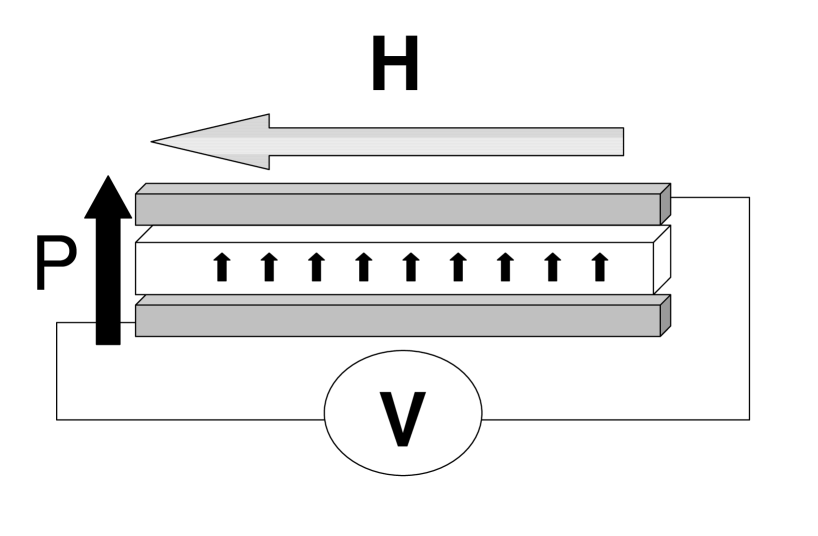
Multiferroics may also have important applications in developing magnetic field sensors. There are a range of proposals for incorporating magnetoelectric materials in exceptionally sensitive magnetic field detectors. Even relatively small external magnetic fields will produce a voltage change in materials with very large magnetoelectric couplings. Since it is often better to measure small voltages at zero applied current rather than small magnetizations or small changes in resistivity, magnetoelectric materials offer the potential for developing greatly improved magnetic field sensors. Because multiferroics exhibiting simultaneous magnetic and ferroelectric transitions offer exceptionally large magnetoelectric couplings, these materials are particularly interesting in the context of improved sensors. Figure 2 shows a schematic for such a device.NASA The magnetization produces a spontaneous polarization directed perpendicular to the plane of the sensor. This magnetically induced voltage can be measured to a high degree of accuracy, either directly, or by measuring the dielectric response of the compound. This device could also be configured to extract energy from an alternating magnetic field—the magnetically induced alternating voltage could be used as a supply for very low power applications.BAYRASHEV

Figure 2: Schematic illustration of a device to measure magnetic fields by using the induced polarization. The middle layer (white) is a multiferroic material with strong magnetoelectric coup0lings and the outer layers (gray) are ferromagnetic metals. In this example the polarization is induced in a direction perpendicular to the applied magnetic field.

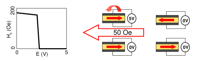
Beyond simply being used as a passive magnetic field sensor, the device illustrated in Fig. 2 could also be configured as a voltage biased magnetic memory element. One of the difficulties facing current magnetic random access memory (MRAM) devices lies in producing sufficiently strong magnetic fields to cause a moment reversal in the memory element, but also sufficiently localized to affect only one specific element. While identifying multiferroic materials in which applying a voltage could reverse the direction of the magnetization would certainly be beneficial for developing MRAM devices, a more modest type of voltage-assisted magnetization reversal could also be significant. As will be discussed in the following section, ferroelectric order can be promoted or suppressed by the application of an external magnetic field in many multiferroic materials. We expect that in these materials, applying an electric field could then suppress or promote magnetic ordering. In such a system, the coercivity of the magnetic memory element could be tuned by applying an electric field. Consider the multiferroic memory element in a ferromagnetic state, which can be suppressed by applying a sufficiently large voltage. In the absence of an electric field, the coercivity of the memory element is large, so the magnetization is unaffected by stray magnetic fields. In order to reverse the magnetization direction, a bias voltage is applied to the multiferroic, bringing the system closer to the magnetic transition, reducing the magnitude of the coercive field. In this state, the magnetization can be reversed by a relatively small external magnetic field, smaller than the coercive field of the unbiased multiferroic. When the voltage is removed, the new magnetization will be stable. This type of voltage-assisted magnetization reversal could be used to produce arrays of magnetic memory elements which could be switched by the same external magnetic field. Only those elements which have a bias voltage applied will have a sufficiently small coercivity to be switched by the magnetic field. This technique may offer advantages over transitional MRAM devices, such as a smaller sensitivity to stray fields (allowing higher bit density) and potentially faster switching times. This is schematically illustrated in Fig. 3.

Figure 3: Voltage-assisted MRAM. Left: Schematic diagram showing how the coercive magnetic field is expected to vary with voltage. Right: With the magnetization of the bits originally directed to the right, a small (50 Oe) writing field is applied. At zero voltage, this is smaller than the coercive field, so that the magnetization does not switch. However, applying 5V across the multiferroic layer reduces the coercive field to almost zero, so that this small magnetic field is sufficient to reverse the direction of magnetization.

III FERROELECTRICITY

We start by making a few observations concerning the symmetry properties of ferroelectric systems for which magnetic ordering plays no role. In the most common scenario, ferroelectrics exhibit a high-temperature phase having spatial inversion symmetry which prevents the existence of a vector order parameter. Then, as the temperature is reduced through a critical value, $T_{F}$, a lattice instability develops in which inversion symmetry is broken cooperatively via a continuous phase transition at which a spontaneous polarization appears. Within a Landau theory this transition is described by a free energy of the form

$$F = {\scriptsize 1\over\scriptsize 2}\chi_{E}^{-1}{\bf P}^{2}+{\cal O}({\bf P})^{4}={\scriptsize 1\over\scriptsize 2}a(T-T_{F}){\bf P}^{2}+{\cal O}({\bf P})^{4}\ .$$ (2)

At the transition the fact that the quadratic term in ${\bf P}$ becomes unstable (negative) reflects the divergence in the electric susceptibility at the ferroelectric transition. This instability is sometimes traced to a soft phonon, but whatever the mechanism, the appearance of ferroelectricity represents a broken symmetry. Conversely, as will become relevant in the following, ferroelectricity can only occur if the symmetry is broken to permit the ordering of the polarization vector. We will use this criterion to determine which types of magnetic order can possibly induce ferroelectric order. If one takes the quartic terms in Eq. (2) to be of the form $a[{\bf P}^{2}]^{2}$ (with $a>0$ for stability), then minimization of $F$ with respect to ${\bf P}$ shows that for $T<T_{F}$ one has $P\sim[2a(T_{F}-T)]^{1/2}$, which is expected to hold as long as $T_{F}-T$ is not so large that sixth and higher order terms in $F$ are important. Mean field theory ignores spatial correlations which lead to modifications of critical exponents, but the scope of this review does not permit consideration of such corrections.PFEUTY

As the temperature is further lowered it is possible for this ferroelectric system to develop long-range magnetic order.LRO In this case, one does not expect significant interaction between electrical and magnetic properties because the two phenomena are essentially independent of one another. In these systems, the spontaneous polarization will depend only weakly on the applied magnetic field. In this scenario, it is well knownFEREF that one can expect anomalies in the dielectric response of the system when the ferroelectric develops (independently) long-range magnetic order. This review is not concerned with such an “accidental” superposition of electric and magnetic properties. Instead we focus our attention on the situation when the appearance of long-range magnetic order induces ferroelectricity. Furthermore, we will consider an interesting subclass in which the long-range magnetic order is modulated with an apparently incommensurate wavevector. We will develop a Landau theory for this combined phase transition in which the fact that the wavevector does not have high-symmetry (and is thus neither ferromagnetic or antiferromagnetic) is crucial to our analysis. Thus the development here can not be obtained by a trivial extension of theories applicable to ferro- or antiferromagnetic ferroelectrics. A simplifying feature of this formulation is that it is based on an expansion of the free energy in powers of the various order parameters relative to the paramagnetic phase. Accordingly, each term in this expansion has to have the full symmetry of the disordered phase.PSYM1 ; PSYM2 In contrast, it is less straightforward to analyze whether or not the symmetry of a magnetically ordered phase permits an induced ferroelectric order. Also, the Landau formulation correctly predicts which components of the spontaneous polarization vector are induced by the magnetic ordering. In addition, the Landau expansion indicates that the spontaneous polarization is, crudely speaking, proportional to the emerging magnetic order parameter.

IV TOY MODELS FOR INCOMMENSURATE MAGNETISM

IV.1 Review of Mean Field Theory

In this section we review the description and phenomenology of incommensurate magnets, because the characterization of their symmetry is essential to understanding the coupling between magnetic and electric long range order.

For the purposes of this review it suffices to consider the description of incommensurate magnets within mean field theory. For a system consisting of quantum spins of magnitude $S$ on each site, we write the trial free energy is

$$F\equiv U-TS={\rm Tr}[{\mbox{\boldmath{$\rho$}}}{\cal H}+kT{\mbox{\boldmath{$\rho$}}}\ln{\mbox{\boldmath{$\rho$}}}]\ ,$$ (3)

where ${\cal H}$ is the Hamiltonian, $T$ the temperature, $U$ the internal energy, $S$ the entropy, and the actual free energy is the minimum of $F$ with respect to the choice of $\rho$ subject to the conditions that $\rho$ is Hermitian with unit trace. Within mean field theory we take the density matrix to be the product of independent single particle density matrices ${\mbox{\boldmath{$\rho$}}}(i)$ for each site $i$:

$${\mbox{\boldmath{$\rho$}}}\equiv\prod_{i}{\mbox{\boldmath{$\rho$}}}(i)\ .$$ (4)

This approximation corresponds to the intuitive idea that when correlations between spins are neglected, each spin reacts to the mean field of its neighbors.

In Eq. (3) the trace of ${\mbox{\boldmath{$\rho$}}}{\cal H}$ gives the internal energy $U$ and that of $-k{\mbox{\boldmath{$\rho$}}}\ln{\mbox{\boldmath{$\rho$}}}$ gives the entropy $S$. In the absence of anisotropy it suffices to set

$${\mbox{\boldmath{$\rho$}}}(i) = {1\over 2S+1}[{\cal I}+c{\mbox{\boldmath{$\sigma$}}}(i)\cdot{\bf S}_{i}]\ ,$$ (5)

where ${\cal I}$ is the unit matrix of dimension $(2S+1)$, $c$ is a constant of order unity, chosen to make Eq. (6) true, and ${\bf S}_{i}$ is the vector spin operator for site $i$ [Here ${\bf S}_{i}$ is a $(2S+1)$ dimensional matrix]. The free energy is then minimized with respect to the trial parameters ${\mbox{\boldmath{$\sigma$}}}(i)$, which physically are identified as the average spin vectors:

$$\langle{\bf S}(i)\rangle\equiv{\rm Tr}[{\mbox{\boldmath{$\rho$}}}(i){\bf S}(i)]={\mbox{\boldmath{$\sigma$}}}(i)\ .$$ (6)

Thus ${\mbox{\boldmath{$\sigma$}}}(i)$ is the vector order parameter at the $i$th lattice site. In this formulation the internal energy is quadratic in the order parameter $\sigma$, whereas the entropic term involves both quadratic and higher powers of the order parameter. As we shall see, even without explicit calculations much information can be inferred from the symmetry of the trial free energy as a function of the order parameter(s).

As mentioned in the introduction, we will focus our attention on systems which display incommensurately modulated magnetic long range order. We refer the reader to a comprehensive survey of such systems by Nagamiya.NAG Here we give a simplified review. To characterize an incommensurate state we consider a toy model consisting of a one dimensional system with isotropic antiferromagnetic exchange interactions $J_{1}$ and $J_{2}$ between nearest and next-nearest neighbors, respectively. If $J_{2}$ is antiferromagnetic and large enough, these two interactions compete and produce an incommensurate spin structure. Thus we are led to consider the Hamiltonian

$${\cal H}=\sum_{n}{\bf S}_{n}\cdot[J_{1}{\bf S}_{n+1}+J_{2}{\bf S}_{n+2}]\ ,$$ (7)

with $J_{2}>0$. The corresponding trial free energy is

$$F = {\scriptsize 1\over\scriptsize 2}dkT\sum_{i}{\mbox{\boldmath{$\sigma$}}}(i)^{2}+\sum_{n=1,2}J_{n}{\mbox{\boldmath{$\sigma$}}}(i)\cdot{\mbox{\boldmath{$\sigma$}}}(i+n)+{\cal O}({\mbox{\boldmath{$\sigma$}}}^{4})\ ,$$ (8)

where the entropic term is scaled by a constant of order unity, $d$.

IV.2 Wavevector Selection

It is instructive to write the free energy per spin, $f$, in terms of Fourier variables, ${\mbox{\boldmath{$\sigma$}}}(q)=(1/N)\sum_{i}e^{iqx_{i}}{\mbox{\boldmath{$\sigma$}}}(i)$, where $N$ is the total number of spins as

$$f \equiv F/N={\scriptsize 1\over\scriptsize 2}\sum_{q}\chi(q)^{-1}{\mbox{\boldmath{$\sigma$}}}(q)\cdot{\mbox{\boldmath{$\sigma$}}}(-q)+{\cal O}({\mbox{\boldmath{$\sigma$}}}^{4})\ ,$$ (9)

where $\chi(q)^{-1}=dkT+J_{1}\cos(qa)+J_{2}\cos(2qa)$ is the wavevector-dependent susceptibility. At high temperature (when $kT\gg|J_{1}|$ and $kT\gg|J_{2}|$), $\chi(q)^{-1}$ is positive for all $q$ and the free energy is minimized by setting all the order parameters ${\mbox{\boldmath{$\sigma$}}}(q)$ to zero. In Fig. 4 we show $\chi(q)^{-1}$ as a function of wavevector $q$ for a sequence of temperatures. As the temperature is lowered through a critical value $T_{c}$, $\chi(q)^{-1}$ becomes zero for the wavevector $q\equiv q_{0}$ which minimizes $\chi(q)^{-1}$:

$$\cos(q_{0}a)=-J_{1}/(4J_{2})\ .$$ (10)

Figure 4: $\chi(q)^{-1}$ at a sequence of temperatures, $T=T_{c}+0.3n$ for $n=0,1,2,3,4,5$ with $J_{1}=1.0$ and $J_{1}/J_{2}=2.56$ (as is appropriate for NVO). Here $T_{c}=0.711$.

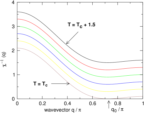
This determination of the value of $q_{0}$ is called wavevector selection. As the temperature is reduced through $T_{c}$ the paramagnetic phase becomes unstable against the formation of long range order at the selected wavevector $q_{0}$. That is, for $T<T_{c}$ the order parameter ${\mbox{\boldmath{$\sigma$}}}(q_{0})$ assumes a nonzero value determined by the (negative) quadratic terms in combination with the (positive) terms of order ${\mbox{\boldmath{$\sigma$}}}^{4}$, so that $|{\mbox{\boldmath{$\sigma$}}}(q_{0})|\sim(T_{c}-T)^{1/2}$. Once order develops at one wavevector, the terms of order ${\mbox{\boldmath{$\sigma$}}}^{4}$ prevent order developing at other wavevectors. This scenario is realistic for a three dimensional system (for which long-range order is not destroyed by thermal fluctuations). The eigenvector associated with the eigenvalue of the quadratic form which passes through zero is called the critical eigenvector. The critical eigenvector contains the form factor of the ordering, i. e. it completely describes the pattern of spin ordering within a unit cell. In this simple model there is only one spin per unit cell, so the eigenvector specifies the direction i. e. the component which condenses. (This concept will be better illustrated when we consider real systems which often have more than one magnetic site per unit cell.) In the present case when there is no anisotropy, the spin structure when ${\mbox{\boldmath{$\sigma$}}}(q)$ becomes nonzero for $q=q_{0}$ is a modulated one in which the $x$-component of spin has a complex amplitude, $A_{x}$, so that

$$\sigma_{x}(i) = A_{x}e^{iq_{0}x_{i}}+A_{x}^{*}e^{-iq_{0}x_{i}}$$ (11)

and similarly for the other spin components. If these complex amplitudes $A_{\alpha}$ all have the same phase,PHASE then the spin is linearly polarized with an amplitude which varies sinusoidally with position. If the complex amplitudes do not have the same phase, then the spin structure will be a helix, a spiral, or a fan, etc.

IV.3 Effects of Anisotropy

This toy model will not accurately capture the behavior of real magnetic systems because we have not yet included any anisotropy. In the presence of single-ion easy axis anisotropy, the trial free energy at quadratic order assumes the form

$$f = {\scriptsize 1\over\scriptsize 2}\sum_{q}\chi(q)^{-1}{\mbox{\boldmath{$\sigma$}}}(q)\cdot{\mbox{\boldmath{$\sigma$}}}(-q)-K\sum_{q}{\mbox{\boldmath{$\sigma$}}}_{x}(q){\mbox{\boldmath{$\sigma$}}}_{x}(-q)+{\cal O}({\mbox{\boldmath{$\sigma$}}}^{4})\ ,$$ (12)

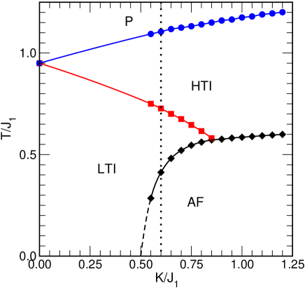
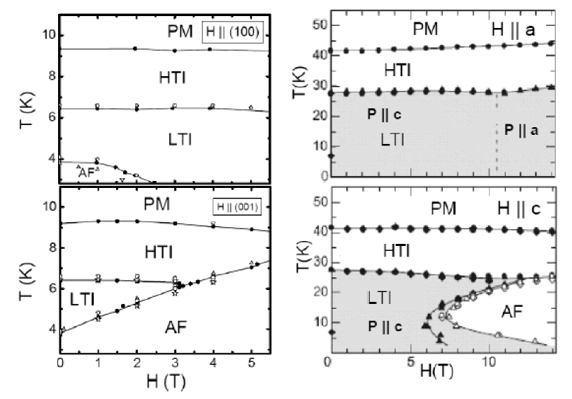
where $K$ is an anisotropy energy which favors alignment of spins along the easy axis, here the $x$-axis, and $f$ denotes the free energy per spin. In this case, the instability (at which long-range order first appears) is one in which the spins are confined to the easy axis and have a sinusoidally varying amplitude. This type of ordered phase will be referred to as the high-temperature incommensurate (HTI) phase and the associated critical temperature will be denoted $T_{\rm HTI}$. If the anisotropy is not too large, then, as the temperature is further reduced, the fourth order terms in the free energy (which we have so far neglected) become important. One effect of these terms can be visualized as incorporating the constraint of “fixed length.” In the HTI phase the spins have a length which varies sinusoidally with position. However, in the ground state, we expect each spin to have its maximum length $S$ but to be oriented in a direction to optimize the energy. Thus, in the extreme limit of zero temperature, the constraint of fixed spin length is fully enforced. Although the constraint is less fully realized at higher temperature, the qualitative effect is clear: when the temperature is sufficiently reduced, one has a continuous phase transition into a phase we refer to as the low-temperature incommensurate (LTI) phase. In this phase the spins develop transverse order (in addition to the preexisting longitudinal order along the easy axis) to more nearly achieve fixed spin length. If the easy axis anisotropy is small, the range of temperature over which the HTI phase is stable is also small. The phase diagram of such a model as a function of anisotropy energy $K$ and temperature is shown in Fig. 5.PRL ; NVO1 We will mainly be concerned with the two incommensurate phases, the longitudinally modulated HTI phase and the elliptically polarized low-temperature incommensurate LTI phase. Although the details of the unit cell complicate the picture, the phenomenology of the HTI and LTI phases are usually roughly similar to that of the simplified case discussed here. In Fig. 6 we show the experimentally determined phase diagrams of NVO and TMO as a function of applied magnetic field $H$ and temperature $T$, with the HTI and LTI phases labelled.

Figure 5: Zero temperature phase diagram for the $J_{1}$-$J_{2}$ ($S=1$) model with easy-axis anisotropy scaled by $K$.NVO1 The points represent numerical implementation of mean-field theory except for $K=0$ where analytic results are used. Here “HTI” denotes a longitudinally polarized incommensurate phase and “LTI” an elliptically polarized incommensurate phase. In both phases the modulation vector is given by Eq. (10). “AF” denotes a two-sublattice collinear antiferromagnetic phase. For large anisotropy this model reduces to the anisotropic nearest next-nearest neighbor Ising (ANNNI) model.ANNNI The dashed line is drawn for a value of the anisotropy energy which reproduces the evolution of magnetic phases in NVO as a function of $T$ for $H=0$.

Figure 6: Phase diagram for NVO (left) and TMO (right) as a function of $H$ and $T$. The HTI and LTI phases will be discussed in more detail below, but correspond roughly to the scenario of our toy model. The interpretation of the $H$-dependence of the phase boundaries for NVO is given in Ref. NVO1, . For NVO the C and C’ phases are commensurate antiferromagnetic phases with a weak ferromagnetic moment. The NVO phase diagram is adapted from Ref. PRL, and the TMO phase diagram is adapted from Ref. TKPRB, .

IV.4 Wavevector Locking

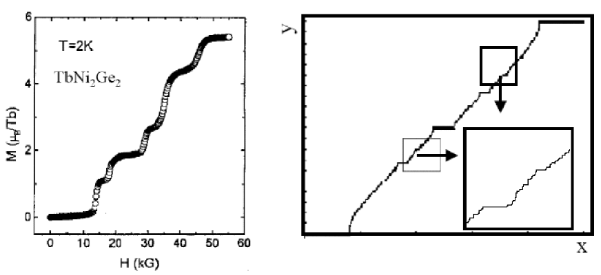
From Eq. (10) it would seem that the wavevector $q$ is a continuous and smooth function of $J_{2}/J_{1}$. Although our toy model does not give any simple explanation for the observed temperature dependence of $q$, a more complete analysis [as in Refs. NVO2, and KAJI, ] leads to a small dependence on temperature which, like the dependence on $J_{2}/J_{1}$, might be thought to be smooth and continuous. However, there are terms which favor commensurate values of $q$. These terms in the free energy must conserve wavevector, but only to within a reciprocal lattice vector $G$ (which for our one-dimensional toy model can assume the values $G_{m}=(2m\pi/a)$, where $a$ is the nearest-neighbor separation). Thus one has the so-called Umklapp terms such as $\delta f=w\sigma(q)^{4}$, when $4q={\bf G}_{m}$. More generally the Umklapp terms give a contribution to the free energy of the form

$$\delta f = \sum_{m,n}w_{m,n}\sigma(q)^{2n}\delta_{nq-2m\pi/a}\ ,$$ (13)

where the coefficient $w_{m}$ is of order unity and $\delta_{x}$ is unity if $x=0$ and is zero otherwise. (Within the present formulation these terms come from expanding ${\rm Tr}{\mbox{\boldmath{$\rho$}}}\ln{\mbox{\boldmath{$\rho$}}}$ to higher than quadratic order in the order parameter.) The effect of these Umklapp terms is to cause the wavevector to “lock” onto a commensurate value $q=2(m/n)\pi/a$ as $J_{2}/J_{1}$ is varied. Since $\sigma(q)$ is smaller than one, especially near the ordering transition, these terms become much less important as the integer denominator $n$ increases. Thus the effect of the Umklapp terms is that the variation of $q$ as a function of a control parameter (such as the temperature) becomes a so-called Devil’s staircase, which may either be complete or (if $\sigma$ is small enough) incomplete, as shown in Fig. 7. In the systems we will discuss here, there is no clear evidence of a Devil’s staircase as a function of temperature. Accordingly, we find it convenient to imagine that $q$ is incommensurate, and does not get stuck on commensurate values by Umklapp terms. Even if this is not strictly true, the difference in properties between an incommensurate system and a commensurate system with a large integer denominator $n$ is experimentally irrelevant for the large values of $n$ ($n\sim 50$), for the systems we will discuss. Accordingly, we will refer to the systems as “incommensurate” even though this may not be strictly accurate.

Figure 7: The Devil’s staircase (DS). Left: an incomplete DS for the dependence of the magnetization of TbNi₂Ge₂ as a function of magnetic field.FIG7 Right: Schematic example of a complete DS function $Y=f(X)$. In a complete DS the function is nonconstant on a set of measure zero. For an incomplete DS the function is nonconstant on a set of nonzero measure.

In principle, the symmetry of real systems is usually such that anisotropy also occurs in the exchange interaction, in which case the trial free energy assumes the form

$$f = {\scriptsize 1\over\scriptsize 2}\sum_{q}\sum_{\alpha=x,y,z}\chi(q)_{\alpha}^{-1}{\mbox{\boldmath{$\sigma$}}}_{\alpha}(q)\cdot{\mbox{\boldmath{$\sigma$}}}_{\alpha}(-q)+{\cal O}({\mbox{\boldmath{$\sigma$}}}^{4})\ ,$$ (14)

where $\chi(q)_{\alpha}^{-1}=dkT+J_{1\alpha}\cos(qa)+J_{2\alpha}\cos(2qa)$. If $J_{n\alpha}$ is isotropic (i.e. if it does not depend on $\alpha$), then the wavevector selected for the ordering of the $\alpha$ component of spin also will not depend on $\alpha$. However, in principle $J_{n\alpha}$ depends weakly on $\alpha$, and therefore the selected wavevector $q_{0}$ will also depend weakly on $\alpha$ and the ordering will involve $\sigma_{x}(q_{x})$, $\sigma_{y}(q_{y})$, and $\sigma_{z}(q_{z})$. Thus in the LTI phase it is possible that the two components of spin might have slightly different wavevectors, which we denote $q_{\rm HTI}$ and $q_{\rm LTI}$. But as with the Umklapp contributions, there will be quartic terms in the free energy (in this formulation coming from the entropic terms) which favor locking the two wavevectors to be equal. These terms can be of the form

$$f_{\rm lock} = a[{\mbox{\boldmath{$\sigma$}}}_{\rm HTI}(q_{\rm HTI})^{2}{\mbox{\boldmath{$\sigma$}}}_{\rm LTI}(-q_{\rm LTI})^{2}+{\mbox{\boldmath{$\sigma$}}}_{\rm HTI}(-q_{\rm HTI})^{2}{\mbox{\boldmath{$\sigma$}}}_{\rm LTI}(q_{\rm LTI})^{2}]\delta_{q_{\rm HTI},q_{\rm LTI}}\ ,$$ (15)

where $\sigma_{\rm HTI}e^{i\phi_{\rm HTI}}\equiv{\mbox{\boldmath{$\sigma$}}}_{\rm HTI}(q_{\rm HTI})$ ($\sigma_{\rm LTI}e^{i\phi_{\rm LTI}}\equiv{\mbox{\boldmath{$\sigma$}}}_{\rm LTI}(q_{\rm LTI})$) is an order parameter characterizing the appearance of the HTI (LTI) phase, and for simplicity we have assumed that the constant $a$ is real-valued. This interaction only satisfies wavevector conservation if the two wavevectors are exactly equal. If, in the absence of this term, the two wavevectors are sufficiently close to one another, then this locking energy will cause the wavevectors of the two order parameters to be locked into equality with one another. (In this case minimization of $\delta f$ will also fix the relative phase $\phi_{\rm HTI}-\phi_{\rm LTI}$.) Since exchange anisotropy is usually not large, the wavevectors associated with different spin components are normally almost equal to one another. In that case $f_{\rm lock}$ will be large enough to lock the HTI and LTI wavevectors to a common value. This “locked” scenario is quite common and we assume it to be the case here. Indeed for the systems discussed below, the data suggests that the HTI and LTI order parameters involve a single wavevector.

V MAGNETIC SYMMETRY

V.1 Nontrivial Unit Cell

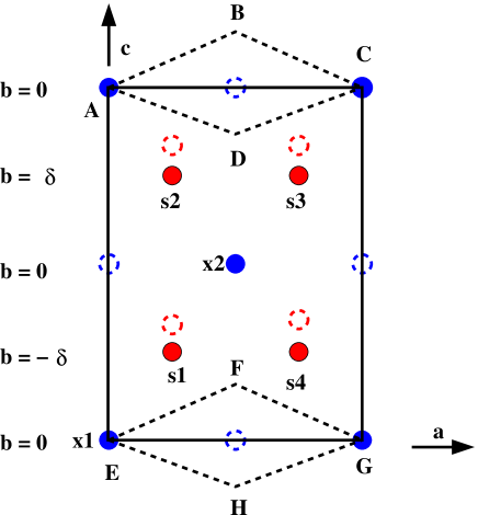
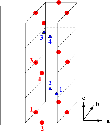
There is one final refinement of our toy model which we must consider, namely the structure of the magnetic unit cell. In the toy model considered above, the entire spin structure is characterized by a wavevector and a single complex vector amplitude. However, more generally, the wavevector determines only how the spin wavefunction evolves from one unit cell to the next. Now we consider how the structure of the wavefunction within a unit cell is restricted by the symmetry of the crystal lattice. As a preliminary, we start by discussing the crystal structure of the two systems, NVO and TMO. In Table 1 we list the general equivalent positions which define the space group operations. For NVO we choose the generators of the space group to be the identity, $E$, a two-fold rotation about the $x$ axis, $(x,y,z)\rightarrow(x,\overline{y},\overline{z})$, the $x-y$ glide plane, $(x,y,z)->(x,y+{\scriptsize 1\over\scriptsize 2},\overline{z}+{\scriptsize 1\over\scriptsize 2})$, spatial inversion, $(x,y,z)\rightarrow(\overline{x},\overline{y},\overline{z})$, and translations. For TMO the generators are taken to be $E$, a mirror $z$-plane, $(x,y,z)\rightarrow(x,y,{\scriptsize 1\over\scriptsize 2}-z)$, the $y-z$ glide plane, $(x,y,z)\rightarrow({\scriptsize 1\over\scriptsize 2}-x,y+{\scriptsize 1\over\scriptsize 2},z)$, spatial inversion, and translations. The magnetic sites are at the positions listed in Table 2 and shown in Fig. 8.

Table 1: General positions of the space groups for NVO (top), Cmca (#64 in Ref. HAHN, ) and for TMO (bottom), Pbnm (#62 in Ref. HAHN, ). For Cmca the primative translation vectors are ${\bf a}_{1}=(a/2)\hat{i}+(b/2)\hat{j}$; ${\bf a}_{2}=(a/2)\hat{i}-(b/2)\hat{j}$; and ${\bf a}_{3}=c\hat{k}$. For Pbnm they are ${\bf a}_{1}=a\hat{i}$; ${\bf a}_{2}=b\hat{j}$, and ${\bf a}_{3}=c\hat{k}$.

${\bf r}=(x,y,z)$	$2_{z}{\bf r}=(\overline{x},\overline{y}+{\scriptsize 1\over\scriptsize 2},z+{\scriptsize 1\over\scriptsize 2})$	$2_{y}{\bf r}=(\overline{x},y+{\scriptsize 1\over\scriptsize 2},\overline{z}+{\scriptsize 1\over\scriptsize 2})$	$2_{x}{\bf r}=(x,\overline{y},\overline{z})$
${\cal I}{\bf r}=(\overline{x},\overline{y},\overline{z})$	$m_{xy}{\bf r}=(x,y+{\scriptsize 1\over\scriptsize 2},\overline{z}+{\scriptsize 1\over\scriptsize 2})$	$m_{xz}{\bf r}=(x,\overline{y}+{\scriptsize 1\over\scriptsize 2},z+{\scriptsize 1\over\scriptsize 2})$	$m_{yz}{\bf r}=(\overline{x},y,z)$

${\bf r}=(x,y,z)$	$m_{xy}{\bf r}=(x,y,{\scriptsize 1\over\scriptsize 2}-z)$	$2_{x}{\bf r}=(x+{\scriptsize 1\over\scriptsize 2},\overline{y}+{\scriptsize 1\over\scriptsize 2},\overline{z})$	$m_{xz}{\bf r}=(x+{\scriptsize 1\over\scriptsize 2},\overline{y}+{\scriptsize 1\over\scriptsize 2},{\scriptsize 1\over\scriptsize 2}+z)$
${\cal I}{\bf r}=(\overline{x},\overline{y},\overline{z})$	$2_{z}{\bf r}=(\overline{x},\overline{y},{\scriptsize 1\over\scriptsize 2}+z)$	$m_{yz}{\bf r}=({\scriptsize 1\over\scriptsize 2}-x,y+{\scriptsize 1\over\scriptsize 2},z)$	$2_{y}{\bf r}=({\scriptsize 1\over\scriptsize 2}-x,y+{\scriptsize 1\over\scriptsize 2},{\scriptsize 1\over\scriptsize 2}-z)$

Table 2: Left: Unit cell lattice positions in NVO of the ${\rm Ni^{2+}}$ ions carrying $S$=$1$ (given as fractions of the cell dimensions $a$, $b$, and $c$). The “spine” sites are $r_{n}^{s}$ and the cross-tie sites are $r_{n}^{c}$. Right: Positions of the Mn and Tb ion sites in the unit cell of TMO as fractions of the cell sides $a$, $b$, and $c$.

$r^{s}_{1}$	(0.25, $-0.13$,0.25)
$r^{s}_{2}$	(0.25, 0.13, 0.75)
$r^{s}_{3}$	(0.75, 0.13, 0.75)
$r^{s}_{4}$	(0.75, $-0.13$, 0.25)
$r^{c}_{1}$	(0, 0, 0)
$r^{c}_{2}$	(0.5, 0, 0.5)

	$n=1$	$n=2$	$n=3$	$n=4$
Mn	(0,${\scriptsize 1\over\scriptsize 2}$ ,0)	$\ \ ({\scriptsize 1\over\scriptsize 2},0,0)\ \$	$\ \ (0,{\scriptsize 1\over\scriptsize 2},{\scriptsize 1\over\scriptsize 2})\ \$	$\ \ ({\scriptsize 1\over\scriptsize 2},0,{\scriptsize 1\over\scriptsize 2})\ \$
Tba	$(x,y,{\scriptsize 1\over\scriptsize 4})$	$(x+{\scriptsize 1\over\scriptsize 2},\overline{y}+{\scriptsize 1\over\scriptsize 2},{\scriptsize 3\over\scriptsize 4})$	$(\overline{x},\overline{y},{\scriptsize 3\over\scriptsize 4})$	$(\overline{x}+{\scriptsize 1\over\scriptsize 2},y+{\scriptsize 1\over\scriptsize 2},{\scriptsize 1\over\scriptsize 4})$

a) $x=0.9836$ and $y=0.0810$ from Ref. TMOSTR, .

Figure 8: Left: The unit cell (ABCDEFGH) showing only Ni ions numbered as in Table 2. The b axis is perpendicular to the plane of the paper. Dashed circles represent spins in adjacent planes displaced from the solid symbols by $\pm{\bf b}/2$. Right: The unit cell of TbMnO₃ showing only the Mn ions (filled circles) and the Tb ions (filled triangles), numbered as in Table 2.

V.2 Representation Theory

If there are $n_{u}$ spins in a unit cell, then an incommensurate state will be described by a wavevector $\bf q$ and the complex-valued Fourier amplitudes ${\cal S}_{\alpha,\tau}({\bf q})$, where $\alpha=x,y,z$ and $\tau=1,2,\dots n_{u}$ , in terms of which we write the spin wavefunctions in the form

$$S_{\alpha,\tau}({\bf R}) = {\cal S}_{\alpha\tau}({\bf q})e^{i{\bf q}\cdot({\bf R}+{\bf r}_{\tau})}+{\cal S}_{\alpha\tau}({\bf q})^{*}e^{-i{\bf q}\cdot({\bf R}+{\bf r}_{\tau})}\ .$$ (16)

where ${\bf r}_{\tau}$ is the position of the $\tau$th site within the unit cell. For NVO $\tau=1,s$; $2,s$; $3,s$; or $4,s$ for spine (s) sites and $1,c$, or $2,c$ for cross-tie (c) sites. Note that the complex amplitudes ${\cal S}(q)$ are defined relative to the phase, ${\bf q}\cdot({\bf R}+{\bf r}_{\tau})$ which would obtain if the wave were perfectly sinusoidal. (This convention will simplify later results.)

We now discuss how symmetry restricts the possible values of the amplitudes ${\cal S}_{\alpha,\tau}(q)$ and how these variables are determined via diffraction experiments. The analysis of the symmetry of such systems in terms of their point groups is not developed. Accordingly, a model-independent (representation) analysisWILLS is customarily invoked in such cases. If the magnetic ordering transition is assumed to be continuous, then the phase transition is signalled by an instability in the quadratic terms when the free energy is expanded in powers of the order parameters. In that case, the spin ordering within a unit cell will be determined by the critical eigenvector associated with the first eigenvalue of the quadratic free energy which passes through zero as the temperature is lowered. This phenomenon has been discussed previously in connection with wavevector selection. As we shall see, this analysis of the magnetic symmetry is essential to construct the allowed couplings between magnetic and ferroelectric order parameters.

In order to conserve wavevector the quadratic terms in the Landau expansion associated with the selected wavevector $\bf q$ must be of the form

$$f_{2} = \sum_{\alpha,\beta,\tau,\tau^{\prime}}c_{\alpha,\tau;\beta,\tau^{\prime}}({\bf q}){\cal S}_{\alpha,\tau}(-{\bf q}){\cal S}_{\beta,\tau^{\prime}}({\bf q})\ ,$$ (17)

where ${\cal S}_{\alpha,\tau}(-{\bf q})={\cal S}_{\alpha,\tau}({\bf q})^{*}$. For $f_{2}$ to be real for any choice of the complex-valued Fourier amplitudes, it is required that $c_{\alpha,\tau;\beta,\tau^{\prime}}({\bf q})^{*}=c_{\beta,\tau^{\prime};\alpha,\tau}({\bf q})$. As in the case of phonons or other normal modes, the eigenvectors of this quadratic form can be labeled according to the irreducible representations (irreps) $\Gamma_{n}$ of the paramagnetic phase which leave the wavevector invariant. (This group of symmetry operations is called the group of the wavevector or the “little group.” The relevant symmetry is that of the paramagnetic phase because the expansion of the free energy in powers of the order parameters is relative to this phase.PSYM1 ; PSYM2 ) For the orthorhombic systems NVO and TMO considered in this review, all the irreps are one dimensional. So essentially, the eigenvectors must be even or odd under the rotation or mirror (or glide) operations of the little group.

The result of the group theoretical analysis is that one expresses the Fourier amplitudes ${\cal S}_{\alpha\tau}({\bf q})$ in terms of symmetry adapted coordinates $m^{(n)}_{\eta}$, associated with the irrep $\Gamma_{n}$. Here the subscript $\eta$ indicates the spin component and type of site within the unit cell. For instance, for NVO, (as we will see later in Table 4), for $n=3$ or $n=4$, $\eta$ ranges over five values, three associated with spin components on spine sites and two associated with spin components on cross tie sites. For $n=1$ or $n=2$, $\eta$ ranges over four values, three associated with spin components on spine sites and one associated with a cross tie spin component. If we write

$${\cal S}_{\alpha\tau}(q) = \sum_{n,\eta}U^{(n)}_{\alpha\tau;\eta}m^{(n)}_{\eta}(q)\ ,$$ (18)

then $U^{(n)}_{\alpha\tau;\eta}$ is the $\eta$th symmetry adapted basis function of irrep $n$ in the sense that it specifies the $\alpha$ spin component for the site $\tau$ in the unit cell. These basis functions are given in Tables 4, 5, and 6, below. (Thus, for condensation of spins in NVO via irrep $\Gamma_{4}$, Table IV indicates that the specification of the magnetic structure requires fixing the five complex-valued symmetry adapted coordinates $m_{sx}^{(4)}$, $m_{sy}^{(4)}$, $m_{sz}^{(4)}$, $m_{cy}^{(4)}$, and $m_{cz}^{(4)}$.) The advantage of this formalism is that the quadratic free energy only couples symmetry adapted coordinates having the same irrep superscript $n$:

$$f_{2} = \sum_{n}\sum_{\eta\eta^{\prime}}F_{\eta,\eta^{\prime}}^{(n)}m_{\eta}^{(n)}(q)^{*}m_{\eta^{\prime}}^{(n)}(q)\ ,$$ (19)

where the reality of $f_{2}$ requires that ${F^{(n)}_{\eta,\eta^{\prime}}}^{*}=F^{(n)}_{\eta^{\prime},\eta}$.

To deal with this free energy it is useful to introduce normal coordinates $\xi^{(n)}_{\rho}$ in terms of which the quadratic form is diagonal. So we set

$$m^{(n)}_{\eta}(q)=\sum_{\rho}u^{(n)}_{\eta\rho}\xi^{(n)}_{\rho}\ ,$$ (20)

and the unitary matrix ${\bf u}^{(n)}$ (which diagonalizes the quadratic free energy) is chosen so that

$$f_{2} = \sum_{n,\rho}\lambda_{\rho}^{(n)}|\xi^{(n)}_{\rho}|^{2}\ .$$ (21)

Usually

$$\lambda_{\rho}^{(n)}=dkT-\tilde{\lambda}_{\rho}{(n)}\ ,$$ (22)

where $\tilde{\lambda}_{\rho}^{(n)}$ is a temperature-independent interaction term. As we shall see, the transformation ${\bf U}$ to symmetry adapted coordinates is determined by the symmetries of the system, whereas the further transformation to normal coordinates depends on the details of the interactions between spins. However, the explicit form of ${\bf u}$ will not be needed for our analysis.

To make this analysis more intuitive we may liken it to the problem of a particle moving in a spherically symmetric potential. For illustrative purposes we consider a Coulomb potential with a weak spherically symmetric perturbation. To solve this problem, one introduces symmetry adapted basis functions for the various irreps, which in this case are s functions $\psi^{(s)}_{n}$, p functions $\psi^{(p_{x})}_{n}$, $\psi^{(p_{y})}_{n}$, $\psi^{(p_{z})}_{n}$, etc. Then $\Psi_{n}^{(q)}$, the $n$th eigenfunction of type $q$ ($q=s$, $q=p_{x}$, etc.) is written in terms of the basis functions as

$$\Psi^{(q)}_{n} = \sum_{m}u^{(q)}_{n\rho}\psi^{(q)}_{\rho}\ .$$ (23)

The basis functions $\psi_{m}^{(q)}$ are constructed solely from symmetry arguments. The actual value of the transformation ${\bf u}$ to eigenfunctions depends on the details of the potential.

We now return to the problem of incommensurate magnets. At high temperature, i. e. in the paramagnetic phase all the eigenvalues $\lambda^{(n)}_{\rho}$ are positive and the trial free energy is minimized by setting $\xi_{\rho}^{(n)}=0$ for all $\rho$ and $n$, so that all the $S_{\alpha\tau}({\bf R})$ are zero: the paramagnetic phase is stable against the formation of long range magnetic order. As the temperature is lowered, one of these eigenvalues will pass through zero [c. f. Fig. 4 and Eq. (22)] and the irrep for which this happens becomes “active,” so to speak. It is conceivable that eigenvalues $\lambda^{(n)}_{\rho}$ and $\lambda^{(n^{\prime})}_{\rho^{\prime}}$ of two different irreps could be degenerate. We reject the possibility of such an accidental degeneracy. However, if one adjusts an additional control parameter, such as the pressure, it is possible to reach a higher order critical point where two irreps simultaneously become active. A simple example of this principle arises when one treats a ferromagnet on a tetragonal lattice. In that case one irrep is one dimensional and corresponds to the ferromagnetic order lying along the four-fold crystal ($\underline{c}$) axis and the other irrep is two-dimensional and corresponds to ordering in the plane perpendicular to the $\underline{c}$ axis. Clearly, the mean-field transition temperatures for these two distinct orderings should be assumed to be different. If the anisotropy is easy-axis the ferromagnetic moment will lie along the $\underline{c}$ axis and if the anisotropy is easy plane the moment will be perpendicular to the $\underline{c}$ axis. It is possible for the anisotropy to vanish, but only by adjusting another thermodynamic variable, such as uniaxial stress. One therefore concludes that criticality is associated with a single irrep. Since the transformation to symmetry adapted coordinates can be determined using only symmetry considerations, the possible patterns of spin ordering within the unit cell are strongly restricted.

In the usual presentation of representational analysis,WILLS the only constraint on the symmetry adapted coordinates is that they transform properly under the operations of the little group, $g_{k}$. For NVO the wavevector in question is along the crystal a axis, and the generators of $g_{k}$ are $2_{x}$, a two-fold rotation about the $x$-axis (we often refer to a, b, and c as $x$, $y$, and $z$, respectively) and $m_{xy}$, a glide operation which takes $z$ into $-z$ followed by a translation of $({\bf b+c})/2$. For TMO the wavevector is along the crystal b axis and the generators of $g_{k}$ are a two-fold screw rotation about the $y$-axis, $2_{y}$ and the mirror plane $m_{xy}$. These operations are defined in Table 1. It should be noted that in the case of TMO the four symmetry operations do not actually form a “group” because $[2_{y}]^{2}$ picks up a phase factor and is thus not equal to a member of the group. This situation also occurs in connection with the application of group theory to the band structure of nonsymmorphic space groups.GROUP ; CORNWELL (These are space groups for which some pure point group operations are not space group operations.) The formal solution to this problem is cumbersome.ZAK Here we may avoid these complications by defining the operator $\tilde{2}_{y}\equiv e^{iqa/2}2_{y}$, so that $[\tilde{2}_{y}]^{2}$ translates the wave into itself. The character tables for these little groups are given in Table 3. (In essence, the character table tells whether wavefunctions associated by $\Gamma_{n}$ are even or odd under the symmetry operations listed.)

Table 3: Character Table for the symmetry operations ${\cal O}$ of the group^(a) $G_{\bf k}$ for the irreps $\Gamma_{n}$ for incommensurate magnetic structure of (left) NVO with ${\bf k}=(q,0,0)$ and (right) TMO for ${\bf k}=(0,q,0)$.

${\cal O}^{({\rm b})}=$	$1$	$2_{x}$	$m_{xy}$	$m_{xz}$
$\Gamma^{1}$	1	1	$1$	$1$
$\Gamma^{2}$	1	1	$-1$	$-1$
$\Gamma^{3}$	1	$-1$	$-1$	$1$
$\Gamma^{4}$	1	$-1$	$1$	$-1$

${\cal O}^{({\rm a})}=$	$E$	$\tilde{2}_{y}$	$m_{xy}$	$\tilde{m}_{yz}$
$\Gamma_{1}$	1	1	$1$	$1$
$\Gamma_{2}$	1	1	$-1$	$-1$
$\Gamma_{3}$	1	$-1$	$1$	$-1$
$\Gamma_{4}$	1	$-1$	$-1$	$1$

a) For an operator ${\cal O}$ we define $\tilde{\cal O}=e^{iqa/2}{\cal O}$.

b) Operators (without tildes) are defined in Table 1.

For either NVO or TMO the next step is to construct the symmetry adapted basis functions which transform according to the irreps listed in Table 3. These allowed symmetry-adapted spin functions are listed in Table 4 for NVO and in Tables 5 and 6 for TMO. (In Table 5 the symmetry adapted coordinates are denoted $M^{\rm M}_{\alpha}$ and in Table 6 they are denoted $M^{\rm T,m}_{\alpha}$.) Note that each symmetry adapted coordinate appearing in these tables is complex-valued, each with an amplitude and (within the analysis discussed up to now) an independent phase. Note also that simply specifying the symmetry does not fix all the spin components in the unit cell. Rather it allows a choice of spin components for each set of symmetry-equivalent sites. For NVO one can specify the spin components of a single spine site and those of a single cross-tie site (unless a component is forced by symmetry to be zero). Having done this, the spin components of the other spine and and cross-tie sites are then fixed by the symmetry properties of the irrep in question.

When the temperature is lowered further and the LTI phase is entered, then an additional irrep will become active via a second continuous phase transition. For NVO the new LTI representation (in addition to $\Gamma_{4}$ already present in the HTI phase) isPRL $\Gamma_{1}$ and for TMO the new LTI representation (in addition to $\Gamma_{3}$ already present in the HTI phase) isTMO $\Gamma_{2}$. In an appendix we discuss that when two different irreps are active, their presence does not induce the development of a third irrep. However, had there been a further phase transition from the LTI phase into yet another incommensurate phase with three irreps, then the presence of three different irreps would induce the presence of a fourth one.

Table 4: Symmetry adapted basis functions $U^{(n)}_{\alpha\tau;\eta}$ which transform according to the irreducible representation $\Gamma_{n}$ for the incommensurate phase associated with ${\bf k}=(q,0,0)$ for the ${\rm Ni}$ spine (s) and cross-tie (c) sites of NVO. Here ${\cal S}_{1s}$ denotes the vector with components ${\cal S}_{x,1s}$, ${\cal S}_{y,1s}$, ${\cal S}_{z,1s}$, and similarly for the other ${\cal S}$’s. The symmetry adapted coordinates $m_{r\alpha}^{(n)}$ assume complex values, as discussed in the text. The numbering of sites is given in Table 2. The phase factors of $i$ are chosen to simplify the transformation properties under spatial inversion, as is discussed below.

	${\bf U}^{(1)}$	${\bf U}^{(2)}$	${\bf U}^{(3)}$	${\bf U}^{(4)}$
${\cal S}_{1s}$	$(im_{sx}^{(1)},m_{sy}^{(1)},im_{sz}^{(1)})$	$(m_{sx}^{(2)},im_{sy}^{(2)},m_{sz}^{(2)})$	$(im_{sx}^{(3)},m_{sy}^{(3)},im_{sz}^{(3)})$	$(m_{sx}^{(4)},im_{sy}^{(4)},m_{sz}^{(4)})$
${\cal S}_{2s}$	$(im_{sx}^{(1)},-m_{sy}^{(1)},-im_{sz}^{(1)})$	$(m_{sx}^{(2)},-im_{sy}^{(2)},-m_{sz}^{(2)})$	$(-im_{sx}^{(3)},m_{sy}^{(3)},im_{sz}^{(3)})$	$(-m_{sx}^{(4)},im_{sy}^{(4)},m_{sz}^{(4)})$
${\cal S}_{3s}$	$(-im_{sx}^{(1)},\,m_{sy}^{(1)},-im_{sz}^{(1)})$	$(\,m_{sx}^{(2)},-im_{sy}^{(2)},\,m_{sz}^{(2)})$	$(-im_{sx}^{(3)},\,m_{sy}^{(3)},-im_{sz}^{(3)})$	$(\,m_{sx}^{(4)}-im_{sy}^{(4)},\,m_{sz}^{(4)})$
${\cal S}_{4s}$	$(-im_{sx}^{(1)},-m_{sy}^{(1)},im_{sz}^{(1)})$	$(\,m_{sx}^{(2)},\,im_{sy}^{(2)},-m_{sz}^{(2)})$	$(\,im_{sx}^{(3)},m_{sy}^{(3)},-im_{sz}^{(3)})$	$(-m_{sx}^{(4)},-im_{sy}^{(4)},\,m_{sz}^{(4)})$
${\cal S}_{1c}$	$(m_{cx}^{(1)},0,0)$	$(m_{cx}^{(2)},0,0)$	$(0,m_{cy}^{(3)},m_{cz}^{(3)})$	$(0,m_{cy}^{(4)},m_{cz}^{(4)})$
${\cal S}_{2c}$	$(-m_{cx}^{(1)},0,0)$	$(\,m_{cx}^{(2)},0,0)$	$(0,m_{cy}^{(3)},-m_{cz}^{(3)})$	$(0,-m_{cy}^{(4)},m_{cz}^{(4)})$

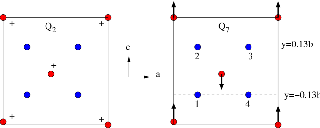
As an illustration of how to apply the above results, we show, in Fig. 9, typical spin configurations for NVO which result from the spin wavefunctions which transform according to irrep #4. The configuration shown in the top panel is not allowed because, as we discuss below, it does not respect inversion symmetry.

Table 5: Symmetry adapted basis functions $U^{(n)}_{\alpha\tau;\eta}$ which transform according to the irreducible representation $\Gamma_{n}$ for the incommensurate phase associated with ${\bf k}=(q,0,0)$ for the Mn sites in TMO. The complex-valued symmetry adapted coordinates are here denoted $M_{\alpha}^{\rm M}$. The sites are numbered as in Table 2.

Mn Site	${\bf U}^{(1)}$	${\bf U}^{(2)}$	${\bf U}^{(3)}$	${\bf U}^{(4)}$
$1$	$(M^{\rm M}_{x},M^{\rm M}_{y},M^{\rm M}_{z})$	$(M^{\rm M}_{x},M^{\rm M}_{y},M^{\rm M}_{z})$	$(M^{\rm M}_{x},M^{\rm M}_{y}M^{\rm M}_{z})$	$(M^{\rm M}_{x},M^{\rm M}_{y},M^{\rm M}_{z})$
$2$	$(M^{\rm M}_{x},-M^{\rm M}_{y},-M^{\rm M}_{z})$	$(-M^{\rm M}_{x},M^{\rm M}_{y},M^{\rm M}_{z})$	$(-M^{\rm M}_{x},M^{\rm M}_{y},M^{\rm M}_{z})$	$(M^{\rm M}_{x},-M^{\rm M}_{y},-M^{\rm M}_{z})$
$3$	$(-M^{\rm M}_{x},-M^{\rm M}_{y},M^{\rm M}_{z})$	$(M^{\rm M}_{x},M^{\rm M}_{y},-M^{\rm M}_{z})$	$(-M^{\rm M}_{x},-M^{\rm M}_{y},M^{\rm M}_{z})$	$(M^{\rm M}_{x},M^{\rm M}_{y},-M^{\rm M}_{z})$
$4$	$(-M^{\rm M}_{x},M^{\rm M}_{y},-M^{\rm M}_{z})$	$(-M^{\rm M}_{x},M^{\rm M}_{y},-M^{\rm M}_{z})$	$(M^{\rm M}_{x},-M^{\rm M}_{y},M^{\rm M}_{z})$	$(M^{\rm M}_{x},-M^{\rm M}_{y},M^{\rm M}_{z})$

Table 6: Symmetry adapted basis functions $U^{(n)}_{\alpha\tau;\eta}$ which transform according to the irreducible representation $\Gamma_{n}$ for the incommensurate phase associated with ${\bf k}=(q,0,0)$ for the Tb sites in TMO. The complex-valued symmetry adapted coordinates are here denoted $M_{\alpha}^{{\rm T},n}$. The sites are numbered as in Table 2.

Tb Site	${\bf U}^{(1)}$	${\bf U}^{(2)}$	${\bf U}^{(3)}$	${\bf U}^{(4)}$
$1$	$(0,0,M^{\rm T,2}_{z})$	$(M^{\rm T,2}_{x},M^{\rm T,2}_{y},0)$	$(0,0,M^{\rm T,2}_{z})$	$(M^{\rm T,2}_{x},M^{\rm T,2}_{y},0)$
$2$	$(0,0,-M^{\rm T,1}_{z})$	$(-M^{\rm T,1}_{x},M^{\rm T,1}_{y},0)$	$(0,0,M^{\rm T,1}_{z})$	$(M^{\rm T,1}_{x},-M^{\rm T,1}_{y},0)$
$3$	$(0,0,M^{\rm T,1}_{z})$	$(M^{\rm T,1}_{x},M^{\rm T,1}_{y},0)$	$(0,0,M^{\rm T,1}_{z})$	$(M^{\rm T,1}_{x},M^{\rm T,1}_{y},0)$
$4$	$(0,0,-M^{\rm T,2}_{z})$	$(-M^{\rm T,2}_{x},M^{\rm T,2}_{y},0)$	$(0,0,M^{\rm T,2}_{z})$	$(M^{\rm T,2}_{x},-M^{\rm T,2}_{y},0)$

Figure 9: Two structures for spine spins in an a -c plane for NVO obtained using spin components from Table 4 which transform according to irrep $\Gamma_{4}$ for wavevector $k=2\pi/(3a)$, where $a/2$ is the distance between sites. The axis for the two-fold rotation $2_{x}$ is indicated. The glide plane, which relates spins in adjacent layers is not shown. The sites are numbered as in Table 2. At the bottom of each panel we give the phase (in degrees) of the wave at each site. Top: for $m_{sx}^{(4)}=1$, $m_{sz}^{(4)}=-i$ and the other parameters equal to zero. Bottom: for $m_{sx}^{(4)}=m_{sz}^{(4)}=1$ and the other parameters equal to zero. As we shall see in Eq. (32), the order parameters $m_{sx}^{(4)}$ and $m_{sz}^{(4)}$ must have the same phase, i. e. $m_{sx}^{(4)}/m_{sz}^{(4)}$ must be real. Only the bottom configuration satisfies this constraint.

V.3 Effect of Inversion Symmetry for NVO

Up to now we only used the consequences of the symmetry of the group of transformations which leave the wavevector invariant. However, as we have observed previously, the quadratic free energy of Eq. (17) or of Eq. (19) must be invariant under all the operations of the paramagnetic space group. In particular, the operations for the systems we consider here which are not in the little group of the wavevector are those generated by spatial inversion ${\cal I}$. We now discuss how inversion symmetry places restrictions on symmetry adapted coordinates. Usually when one introduces an additional symmetry, the matrix for the quadratic free energy becomes block diagonal. Here, the result of the additional symmetry is not to reduce the size of the submatrices for the quadratic free energy, but rather it places additional constraints on the transformation matrix ${\bf u}$ of Eq. (20). As we shall see, when ${\bf U}$ is appropriately defined, then inversion symmetry restricts all the matrix elements $F^{(n)}_{\eta,\eta^{\prime}}$ to be real. Consequently ${\bf u}$ is real, apart from an overall phase $\phi_{n}$ which is associated with each irrep $\Gamma_{n}$.

We first analyze the situation for NVO. We need to determine the effect of ${\cal I}$ on the spin wavefunctions listed in Table 4. Recall that the magnetic moment is a pseudovector. That means that under spatial inversion the orientation of the moment is unchanged, but it is simply transported from its initial location at ${\bf r}$ to the transformed location, $-{\bf r}$. Looking at Eq. (16) we see that spatial inversion interchanges ${\cal S}$ and ${\cal S}^{*}$, but since the orientation is unchanged, spatial inversion will not affect the spin component label $\alpha$. However, spatial inversion does interchange Ni sublattices #1 and #3 and also #2 and #4. In other words, in the notation of Table 4, we have

$${\cal I}{\cal S}_{x,s1}={\cal S}_{x,s3}^{*}\ ,\ \ \ {\cal I}{\cal S}_{x,s2}={\cal S}_{x,s4}^{*}\ .$$ (24)

To see the consequences of these relations, consider the effect of the first of these two relations acting on the basis functions of ${\bf U}^{(1)}$, for instance. This relation is

$${\cal I}(im_{sx}^{(1)},m_{sy}^{(1)},im_{sz}^{(1)})=(-im_{sx}^{(1)},m_{sy}^{(1)},-im_{sz}^{(1)})^{*}\ ,$$ (25)

which can be written as

$${\cal I}(m_{sx}^{(1)},m_{sy}^{(1)},m_{sz}^{(1)})=(m_{sx}^{(1)},m_{sy}^{(1)},m_{sz}^{(1)})^{*}\ .$$ (26)

This same analysis can be repeated for the other representations and also for the second relation of Eq. (24). Then we see that the choices of the phase factors $i$ in Table 4 leads to the simple result that for $\alpha=x,y,$ or $z$, and independent of representation $\Gamma_{n}$

$${\cal I}{\bf m}_{s\alpha}^{(n)}(q) = {\bf m}_{s\alpha}^{(n)}(q)^{*}\ .$$ (27)

For the cross tie sites, the situation is similar except that under spatial inversion each sublattice is transformed into itself. Thus, we find that

$${\cal I}{\bf m}_{c\alpha}^{(n)}(q)={\bf m}_{c\alpha}^{(n)}(q)^{*}\ .$$ (28)

So, generally for NVO we have for any representation $\Gamma_{n}$

$${\cal I}m_{\eta}^{(n)}(q)=m_{\eta}^{(n)}(q)^{*}\ ,$$ (29)

where $\eta=s,\alpha$ or $\eta=c,\alpha$, where $\alpha=x,y,z$. (Note that this relation does not imply inversion symmetry. If the system has inversion symmetry about the origin, then ${\cal I}m_{\eta}^{(n)}(q)=m_{\eta}^{(n)}$, and magnetic order can not induce ferroelectric order. Thus one can not have ferroelectric order if all the $m$’s are real.)

Now we return to the Landau expansion of Eq. (19) to see how these relations affect the determination of the critical eigenvectors. First consider the situation for NVO when one has Eq. (29). Recall that

$$F^{(n)}_{\eta,\eta^{\prime}}=[F^{(n)}_{\eta^{\prime},\eta}]^{*}\ .$$ (30)

Now we use Eq. (29) to see the consequences of the invariance of $f_{2}$ with respect to inversion symmetry. we again use the fact that $f_{2}$ must be invariant under the symmetry operations of the paramagnetic phase,PSYM1 ; PSYM2 and spatial inversion is one such symmetry. We find that

$${\cal I}f_{2} = \sum_{n}\sum_{\eta\eta^{\prime}}F^{(n)}_{\eta,\eta^{\prime}}[{\cal I}m_{\eta}^{(n)}(q)^{*}][{\cal I}m_{\eta^{\prime}}^{(n)}(q)]=\sum_{n}\sum_{\eta\eta^{\prime}}F^{(n)}_{\eta,\eta^{\prime}}m_{\eta}^{(n)}(q)m_{\eta^{\prime}}^{(n)}(q)^{*}$$ (31)

$$= \sum_{n}\sum_{\eta\eta^{\prime}}F^{(n)}_{\eta^{\prime},\eta}m_{\eta}^{(n)}(q)^{*}m_{\eta^{\prime}}^{(n)}(q)\ .$$

Thus we see that inversion invariance of $f_{2}^{(n)}$ implies that $F^{(n)}_{\eta,\eta^{\prime}}=F^{(n)}_{\eta^{\prime},\eta}$. Combining this with Eq. (30) we see that these coefficients must all be real valued. This means that all the components of the eigenvectors of the quadratic free energy, when written in terms of the variables of Eq. (19), can be taken to be real valued. This does not mean that these variables must be real. Rather, since these variables are allowed to be complex, one may introduce an overall complex phase factor. So, the critical eigenvector, which we denote $u^{(4)}_{\eta,\rho}$ with $\rho=0$, has an arbitrary overall phase, in which case the amplitudes in the HTI phase are given as

$$m_{\eta}^{(4)} = \sigma_{\rm HTI}u^{(4)}_{\eta,0}=\sigma_{\rm HTI}e^{i\phi_{\rm HTI}}r^{(4)}_{\eta,0}\ ,$$ (32)

in terms of the real-valued eigenvalue components $r_{\eta,0}^{(4)}$. Because we have just found that the matrix ${\bf F}^{(n)}$ is real (and symmetric), the components of the eigenvector $r_{\eta,0}$ are real valued, but, as mentioned above, since they depend on the details of the interactions, we do not say anything about their explicit form. Also, because we have introduced an overall scale factor $\sigma_{\rm HTI}$, we may require that $\sum_{\eta}[r^{(4)}_{\eta,0}]^{2}=1$. Equation (32) shows that we are dealing with an $x-y$ like order parameter ${\mbox{\boldmath{$\sigma$}}}\equiv\sigma_{\rm HTI}e^{i\phi_{\rm HTI}}$ which has an amplitude and a phase. (As the temperature is varied near $T_{\rm HTI}$, Landau theory gives the approximate result $\sigma_{\rm HTI}\sim(T_{\rm HTI}-T)^{1/2}$.) In the appendix this argument (showing that the $u^{(n)}_{\eta,\rho}$ are real apart from an overall phase factor) is extended to include fourth order terms in the free energy. In analyzing experimental data, it is very helpful to realize that apart from the overall phase, $\phi_{\rm HTI}$, all the phases of the spin amplitudes are fixed. When speaking in terms of the spin components, ${\cal S}_{\alpha\tau}(q)$, the listing of Table 4 indicates that (for irrep #4, for instance), ${\cal S}_{x,1s}(q)$, ${\cal S}_{z,1s}(q)$, ${\cal S}_{y,1c}(q)$, and ${\cal S}_{z,1c}(q)$ will all have the same phase, but (due to the factor $i$), ${\cal S}_{y,1s}(q)$ will be out of phase with the other variables. As it happens, unless a huge number (several thousand) of reflections are monitored, it is impossible to use diffraction data to fix the relative phases with any degree of certainty. Thus, this theoretical development is useful to completely determine the spin structure of complicated systems such as NVO or TMO.

We now check to see whether or not the HTI phase has a center of inversion symmetry, in which case, a spontaneous polarization can not be induced in this phase. We will show that a phase with a single representation has inversion symmetry. First of all, because we assume incommensurability, we can redefine the origin to be arbitrarily close to a lattice site at $R$, such that $\phi-qR$ is a multiple of $2\pi$. We have already noted that ${\cal I}m_{\alpha}^{\tau}={m_{\alpha}^{\tau}}^{*}$. But if $\phi$ is redefined to be zero, this implies that ${\cal I}m_{\alpha}^{\tau}=m_{\alpha}^{\tau}$, which means that the spin structure has inversion symmetry about the redefined origin. In Fig. 9 we show an example of a system obeying Eq. (32) which does have inversion symmetry and one having an arbitrary set of parameters out of Table 4 which does not satisfy Eq. (32). This latter structure does not display inversion symmetry. Note that, as exemplified by the bottom panel of Fig. 9, it is possible for a structure to be noncollinear, but to have a center of inversion symmetry. So noncollinearity, in and of itself, does not guarantee having a spontaneous polarization.

The analysis of the LTI phase is similar. Here again one can use the transformation properties of the order parameters under inversion to fix the phases of the spin amplitudes. Again, at quadratic order, one has the same result as for the HTI phase: all the LTI order parameters $m_{\alpha}^{s}$ for the LTI irrep have the same phase. The analysis is extended to quartic order in the appendix.

V.4 Effect of Inversion Symmetry for TMO

For TMO each Mn sublattice is transformed into itself, so for the parameters of Table 5 we have

$${\cal I}M^{\rm M}_{\alpha}(q)=M^{\rm M}_{\alpha}(q)^{*}\ .$$ (33)

For the Tb spins, inversion transforms sublattice #1 into #3 and #2 into #4, so that for them one has

$${\cal I}M^{{\rm T},n}_{\alpha}(q)=M^{{\rm T},3-n}_{\alpha}(q)^{*}\ ,$$ (34)

where $n=1,2$ and $\alpha=x,y$, or $z$. [${\rm M}_{\alpha}^{{\rm T},1}(q)$ is associated with sites #1 and #4 and ${\rm M}_{\alpha}^{{\rm T},2}(q)$ is associated with sites #2 and #3.]

The situation for TMO is slightly more complicated than it was for NVO because of the presence of the lower-symmetry Tb sites. In the HTI phase one can repeat the argument used for NVO to show that all the spin components on the Mn sites, $M_{\alpha}^{\rm M}$, have the same phase. In the HTI phase the irrep for TMO was determined to be $\Gamma_{3}$. Accordingly we study the quadratic free energy $f_{2}^{(3)}$ associated with a single irrep, $\Gamma_{3}$. In matrix notation we have the quadratic free energy in terms of symmetry adapted coordinates as

$$f_{2}^{(3)} = \left[M_{x}^{*},M_{y}^{*},M_{z}^{*},T_{1}^{*},T_{2}^{*}\right]\left[\begin{array}[]{c c c c c}a&b&c&z_{1}&z_{2}\\ b&d&e&z_{3}&z_{4}\\ c&e&f&z_{5}&z_{6}\\ z_{1}^{*}&z_{3}^{*}&z_{5}^{*}&g&z_{7}\\ z_{2}^{*}&z_{4}^{*}&z_{6}^{*}&z_{7}^{*}&h\\ \end{array}\right]\left[\begin{array}[]{c}M_{x}\\ M_{y}\\ M_{z}\\ T_{1}\\ T_{2}\\ \end{array}\right]\ .$$ (45)

where $M_{\alpha}$ denotes the Mn amplitude $M_{\alpha}^{\rm M}$, and $T_{1}$ and $T_{2}$ denotes the Tb amplitudes, $M_{z}^{T,1}$ and $M_{z}^{T,2}$, respectively (all for $\Gamma_{3}$). In writing this form we have used the fact that the reality of $f_{2}^{(3)}$ requires the matrix to be Hermitian. Also the matrix elements $a$-$h$ are real, as can be shown from the arguments used previously for NVO. We now consider complex-valued matrix elements $z_{n}$, which have no analog for NVO.ANALOG We see that the form of Eq. (45) implies a contribution to $f_{2}^{(3)}$ of the form $z_{1}M_{x}^{*}T_{1}$. Using inversion symmetry this term can also be written as $z_{1}T_{2}^{*}M_{x}$. Comparing this result to that of Eq. (45) we see that $z_{2}^{*}=z_{1}$. Similarly one can show that $z_{4}^{*}=z_{3}$ and $z_{6}^{*}=z_{5}$. Inversion symmetry gives no information on the phase of $z_{7}$. Thus the matrix for $f_{2}^{(3)}$ is of the form

$$\left[\begin{array}[]{c c c c c}a&b&c&y_{1}&y_{1}^{*}\\ b&d&e&y_{2}&y_{2}^{*}\\ c&e&f&y_{3}&y_{3}^{*}\\ y_{1}^{*}&y_{2}^{*}&y_{3}^{*}&g&y_{4}\\ y_{1}&y_{2}&y_{3}&y_{4}^{*}&h\\ \end{array}\right]\ .$$ (51)

One can then show that any eigenvector of this matrix must be of the form

$$\psi = [M_{x},M_{y},M_{z},T_{1},T_{2}]=\sigma_{\rm HTI}[r_{x},r_{y},r_{z},c,c^{*}]e^{i\phi_{\rm HTI}}\ ,$$ (52)

where $r_{\alpha}$ is real, $c$ can be complex, and we require the normalization $\sum r_{\alpha}^{2}+2|c|^{2}=1$. As for NVO, we introduced an arbitrary overall phase $\phi_{\rm HTI}$. Note that $M_{\alpha}^{\rm M}(q)=\sigma_{\rm HTI}r_{\alpha}e^{i\phi_{\rm HTI}}$, $M_{z}^{{\rm T},1}(q)=\sigma_{\rm HTI}ce^{i\phi_{\rm HTI}}$ and $M_{z}^{{\rm T},2}(q)=\sigma_{\rm HTI}c^{*}e^{i\phi_{\rm HTI}}$. Thus, as a result of inversion symmetry, the amplitudes of the two Tb sublattices are equal in magnitude, and have equal and opposite relative phases (from $c$ and $c^{*}$), the value of which is not fixed by symmetry. As for NVO, one can verify that $\psi$ is inversion invariant if $\phi$ is redefined to be zero, since then ${\cal I}r_{\alpha}=r_{\alpha}$ and ${\cal I}c=(c^{*})^{*}=c$.

V.5 Summary

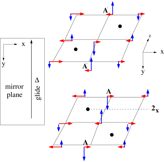
Finally, we should emphasize that although we do not have a quantitative treatment of the development of magnetic long range order, we can certainly determine the magnetic symmetry. This information is encoded in Table 3. For NVO, $\sigma_{\rm HTI}$ is associated with irrep #4 and therefore is odd under a two-fold rotation about $x$ and even with respect to the mirror plane taking $z$ into $-z$. Likewise $\sigma_{\rm LTI}$ is associated with irrep #1 and is therefore even with respect to both these operations. For future reference we also give the transformation properties of ${\mbox{\boldmath{$\sigma$}}}_{\rm HTI}{\mbox{\boldmath{$\sigma$}}}_{\rm LTI}$. These results are summarized in Table 7. The symmetry of the LTI phase of NVO is illustrated in Fig. 10.

Table 7: Transformation Properties of Order Parameters for NVO (left) and TMO (right). In this table ${\mbox{\boldmath{$\sigma$}}}\equiv\sigma e^{i\phi}$. and “c.c.” denotes complex conjugation. Each column gives the result of applying the operator at the top of the column to the order parameter listed in the row.

Order Parameter	$2_{x}$	$m_{xy}$	${\cal I}$
${\mbox{\boldmath{$\sigma$}}}_{\rm HTI}(q)$	$-1$	$1$	c.c.
${\mbox{\boldmath{$\sigma$}}}_{\rm LTI}(q)$	$1$	$1$	c.c.
${\mbox{\boldmath{$\sigma$}}}_{\rm LTI}(q){\mbox{\boldmath{$\sigma$}}}_{\rm HTI}(-q)$	$-1$	$1$	c.c.

Order Parameter	$\tilde{2}_{y}$	$m_{xy}$	${\cal I}$
${\mbox{\boldmath{$\sigma$}}}_{\rm HTI}(q)$	$-1$	$1$	c.c.
${\mbox{\boldmath{$\sigma$}}}_{\rm LTI}(q)$	$1$	$-1$	c.c.
${\mbox{\boldmath{$\sigma$}}}_{\rm LTI}(q){\mbox{\boldmath{$\sigma$}}}_{\rm HTI}(-q)$	$-1$	$-1$	c.c.

Table 8: Values of the symmetry adapted parameters which describe the HTI and LTI phases of NVO^a and TMO.^b The uncertainty in the last digit quoted is given in parenthesis. Where there is no parenthesis, the entry is fixed by symmetry to be zero. For TMO the two Tb order parameters were assumed to have the same magnitude (as predicted by Landau theory) and the phase difference between the two Tb parameters in the LTI phase was found to be $1.3(3)\pi$. For NVO $T=7$K is in the HTI phase and $T=5$K is in the LTI phase. For TMO $T=35$K is in the HTI phase and $T=15$K is in the LTI phase.

NVO					TMO
$T$(K)	Variable	$\alpha=x$	$\alpha=y$	$\alpha=z$	$T$(K)	Variable	$\alpha=x$	$\alpha=y$	$\alpha=z$
7	$m_{\alpha s}^{(4)}$	1.93(5)	0.20 (5)	0.10 (4)	35	$M^{{\rm M},3}_{\alpha}$	0.0(8)	2.90(5)	0.0 (5)
7	$m_{\alpha c}^{(4)}$	0	$-$0.2 (2)	0.00 (2)	35	$M^{{\rm T},3}_{\alpha}$	0	0	0.0 (4)
5	$m_{\alpha s}^{(4)}$	2.0(1)	0.16 (9)	0.01 (5)	15	$M^{{\rm M},3}_{\alpha}$	0.0(5)	3.9(1)	0.0 (7)
5	$m_{\alpha s}^{(1)}$	0.5 (5)	$-$0.5 (1)	0.00 (3)	15	$M^{{\rm M},2}_{\alpha}$	0.0(1)	0.0(8)	2.8 (1)
5	$m_{\alpha c}^{(4)}$	0	$-$2.1 (2)	$-$0.03 (9)	15	$M^{{\rm T},3}_{\alpha}$	0	0	0 (1)
5	$m_{\alpha c}^{(1)}$	0.9 (5)	0	0	15	$M^{{\rm T},2}_{\alpha}$	1.2(1)	0(1)	0

a) See Ref. PRL, .                                                           b) See Ref. TMO, .

For TMO the HTI order parameter ${\mbox{\boldmath{$\sigma$}}}_{\rm HTI}$ is odd with respect to the mirror taking $z$ into $-z$ and is even with respect to the mirror taking $x$ into $-x$. Likewise ${\mbox{\boldmath{$\sigma$}}}_{\rm LTI}$ is associated with irrep #2 and is even with respect to the mirror taking $z$ into $-z$ and is odd with respect to the mirror taking $x$ into $-x$ and these results are summarized in Table 7.

In Table 8 we give the experimentally determined values of the symmetry adapted parameters that describe the HTI and LTI phases of NVO and TMO. The results for NVO are analyzed in detail in Refs. NVO1, and NVO2, . We will make a few brief observations here. For NVO the spine spins dominantly have order in the $x$-direction in the HTI phase from irrep $\Gamma_{4}$ indicating that the $x$-axis is the easy axis. The additional order in the LTI phase due to irrep $\Gamma_{1}$ is along the $y$-direction, as illustrated in Fig. 10. From this figure one sees that interactions between nearest neighboring spins in adjacent spines displaced from one another along either ${\bf c}$ or ${\bf b}$ are antiferromagnetic. Since the wavevectors are the same for both types of order, we infer that the exchange interactions are nearly isotropic. For the Mn spins in TMO the situation is much the same. In the HTI phase, the Mn spins dominantly have order in the $y$ direction, indicating that this axis is the easy axis. In the HTI irrep ($\Gamma_{3}$) one sees, from Table 5, that sites #1 and #2 (in one basal plane) have positive $y$-components of spin and that sites #3 and #4 (in the adjacent basal plane) have negative $y$-components of spin indicating ferromagnetic in-plane interactions and antiferromagnetic out-of-plane interactions. In the LTI phase of TMO, the additional irrep $\Gamma_{2}$ involves spins along $z$-axis and Table 5 shows that for irrep #2 the components are again arranged ferromagnetically within basal planes but antiferromagnetically between adjacent basal planes. The fact that both components of spin are organized similarly suggests that the exchange interactions are probably nearly isotropic.

Figure 10: Schematic representation to show the symmetry of spin components for NVO. Here we show sections of two adjacent ${\bf a}$-${\bf c}$ planes. The filled circles indicate the cross-tie sites whose spin components are not shown, for simplicity. The $x$ components transform according $\Gamma_{4}$: they are odd under the two-fold rotation $2_{x}$ about the $x$-axis and are even under the $x-y$ glide plane (the mirror plane is shown at left with a subsequent displacement $\vec{\Delta}$ along $\hat{y}$). (Remember that the magnetic moment vector involves a cross product and therefore is an axial vector: under a mirror operation it picks up an extra minus sign.) The $y$ components transform according to $\Gamma_{1}$: they are even under both operations. Although the $x$ and $y$ components have different symmetry, they can plausibly result from nearly isotropic exchange interactions.

VI Magnetoelectric Coupling

VI.1 Landau Theory with Two Order Parameters

Now we consider the Landau expansion for the free energy, $f_{ME}$, of the combined magnetic and electric system. One might be tempted to write

$$f_{ME} = a(T-T_{F}){\bf P}^{2}+b(T-T_{M})|\sigma|^{2}\ ,$$ (53)

where $\sigma$ is a magnetic order parameter and, if we wish to describe a phase transition in which both electric and magnetic order appear simultaneously, we would set $T_{F}=T_{M}$. There are several reasons to reject this scenario. First of all, it is never attractive to assume an accidental degeneracy ($T_{F}=T_{M}$). This degeneracy can happen, of course, but normally one would have to adjust some addition control parameter (such as pressure) to reach such a higher order critical point. In addition, in this type of scenario magnetic and electric properties would not be interrelated. In NVO and TMO, in contrast, as shown in Fig, 1, the electric polarization has a dramatic dependence on the applied magnetic field,RAPID which such an independent scenario could not explain.

VI.2 Landau Theory with Two Coupled Order Parameters

Accordingly, we turn to a formulation in which the appearance of magnetic order induces ferroelectric order. (The possibility that electric order induces magnetic order is not allowed by symmetry, by the argument in footnote 87 of Ref. toledano, .) So we write

$$f_{ME} = a\chi_{E}^{-1}{\bf P}^{2}+a(T-T_{M})|\sigma|^{2}+V_{ME}\ ,$$ (54)

where $\chi_{E}^{-1}$ does not approach zero and the simultaneous appearance of magnetic and electric order is due to the term $V_{ME}$. As we have seen, the magnetic order is associated with a nonzero wavevector, whereas the ferroelectric order is a zero wavevector phenomenon. Accordingly, we are constrained to posit a magnetoelectric coupling of the form

$$V_{ME} \sim \sigma(q)\sigma(-q)P\ .$$ (55)

This term will do what we want: when magnetic order appears in $\sigma(q)$, it will then give rise to a linear perturbation in $P$, so that $P\sim\chi_{E}|\sigma(q)|^{2}$. This argument is schematic, of course, and we will have to fill in the details, which must be consistent with the crystal symmetry of the specific systems involved.

The minimal phenomenological model which describes the magnetic and electric behavior of the HTI and LTI phases is therefore written as

$$f = {\scriptsize 1\over\scriptsize 2}(T-T_{\rm HTI}){\mbox{\boldmath{$\sigma$}}}_{\rm HTI}(q){\mbox{\boldmath{$\sigma$}}}_{\rm HTI}^{*}(q)+{\scriptsize 1\over\scriptsize 2}(T-T_{\rm LTI}){\mbox{\boldmath{$\sigma$}}}_{\rm LTI}(q){\mbox{\boldmath{$\sigma$}}}_{\rm LTI}^{*}(q)$$ (56)

$$\ \ +{\cal O}(|\sigma|^{4})+{\scriptsize 1\over\scriptsize 2}\chi_{E}^{-1}{\bf P}^{2}+V_{ME}\ ,$$

where

$$V_{ME} = \sum_{\rm A,B=LTI,HTI}\sum_{\gamma=x,y,z}a_{A,B,\gamma}{\mbox{\boldmath{$\sigma$}}}_{A}(q)^{*}{\mbox{\boldmath{$\sigma$}}}_{B}(q)P_{\gamma}\ .$$ (57)

VI.3 Symmetry of Magnetoelectric Coupling

We now show that this free energy reproduces the observed phenomenology of ferroelectricity in NVO and TMO. First, of all, in the HTI phase (where ${\mbox{\boldmath{$\sigma$}}}_{\rm LTI}=0$) $V_{ME}$ is of the form

$$V_{ME} = \sum_{\gamma}b_{\gamma}|{\mbox{\boldmath{$\sigma$}}}_{\rm HTI}(q)|^{2}P_{\gamma}\ ,$$ (58)

where $b_{\gamma}$ is real. Now we use the fact that $V_{ME}$ has to be inversion-invariant, since it arises in an expansion relative to the paramagnetic phase, which is inversion-invariant.PSYM1 ; PSYM2 We use ${\cal I}\sigma_{\rm HTI}(q)=\sigma_{\rm HTI}(q)^{*}$ and ${\cal I}P_{\gamma}=-P_{\gamma}$ to show that $b_{\gamma}$ must vanish. Indeed, we have already seen, the HTI phases of NVO and TMO are inversion invariant. So for these situations $b_{\gamma}$ in Eq. (58) must be zero and no polarization can be induced in the HTI phase.

Now we consider the situation in the LTI phase when the two order parameters $\sigma_{\rm HTI}$ and $\sigma_{\rm LTI}$ are both nonzero. The argument which indicated that $a_{{\rm HTI},{\rm HTI},\gamma}=0$ can be used to establish that $a_{{\rm LTI},{\rm LTI},\gamma}=0$. Then we write

$$V_{ME} = \sum_{\gamma}[c_{\gamma}{\mbox{\boldmath{$\sigma$}}}_{\rm HTI}(q)^{*}{\mbox{\boldmath{$\sigma$}}}_{\rm LTI}(q)+c_{\gamma}^{*}{\mbox{\boldmath{$\sigma$}}}_{\rm LTI}^{*}(q){\mbox{\boldmath{$\sigma$}}}_{\rm HTI}(q)]P_{\gamma}\ .$$ (59)

This interaction has to be inversion invariant, so we use the transformation properties of the order parameters under inversion to write

$$V_{ME} = {\cal I}V_{ME}=-\sum_{\gamma}[c_{\gamma}{\mbox{\boldmath{$\sigma$}}}_{\rm HTI}(q){\mbox{\boldmath{$\sigma$}}}_{\rm LTI}(q)^{*}+c_{\gamma}^{*}{\mbox{\boldmath{$\sigma$}}}_{\rm LTI}(q){\mbox{\boldmath{$\sigma$}}}_{\rm HTI}(q)^{*}]P_{\gamma}\ .$$ (60)

Comparison with Eq. (59) indicates that $c_{\gamma}$ must be pure imaginary: $c_{\gamma}=ir_{\gamma}$, where $r_{\gamma}$ is real. Then

$$V_{ME} = 2\sum_{\gamma}r_{\gamma}\sigma_{\rm HTI}(q)\sigma_{\rm LTI}(q)P_{\gamma}\sin[\phi_{\rm HTI}-\phi_{\rm LTI}]\ .$$ (61)

This result shows that to get a nonzero spontaneous polarization it is necessary that two order parameters be nonzero. (A similar interaction was proposed by Frohlich et al.TWO in their analysis of second harmonic generation.) Furthermore, these two order parameters must not have the same phase. In fact, a more detailed analysis of Landau theory shows that the phase difference $\phi_{\rm HTI}-\phi_{\rm LTI}$ is expected to be $\pi/2$. (This result comes from an analysis of the quartic terms. As we observed earlier, the function of the quartic terms is to enforce the constraint of fixed spin length. This constraint usually means that the ordering in two representations should be out of phase, so that when one representation gives a maximum of spin lengths, the other gives a minimum of spin lengths.)

Finally, we consider how the symmetry properties constrain the spontaneous polarization. Look at Table 7. There we see how the magnetic order parameters transform under the various symmetry operations of the paramagnetic phase. For $V_{ME}$ to be an invariant, we see that for NVO, ${\bf P}$ must be odd under $2_{x}$ (which restricts ${\bf P}$ to be along $y$ or $z$) and it must be even under $m_{xy}$ (which restricts ${\bf P}$ to be along $x$ or $y$). Thus, symmetry restricts ${\bf P}$ to be only along $y$. This is exactly what experiment shows. For TMO, ${\bf P}$ must be odd under both $\tilde{2}_{y}$ and $m_{xy}$. Thus, symmetry restricts ${\bf P}$ to lie along $z$ at $H=0$, as is observed in experiment. (At higher magnetic fields the magnetic symmetry must change to explain why the polarization switches from the $z$-axis to the $x$-axis.) Furthermore, the temperature variation of ${\bf P}$, shown in Fig. 11 looks very much like that for an order parameter. But that is to be expected because if we minimize the total free energy with respect to ${\bf P}$, using Eq. (61), we see that the spontaneous polarization is given as

$$P_{\gamma}\sim\chi_{E}\sigma_{\rm HTI}\sigma_{\rm LTI}\ .$$ (62)

When the LTI phase is entered, $\sigma_{\rm HTI}$ is already well developed and is therefore essentially independent of temperature. Thus we expect that crudely $P_{\gamma}\sim\sigma_{\rm LTI}$. Indeed, although we have not undertaken a quantitative analysis, the experimental curves of $P$ versus $T$ look quite similar to those for an order parameter.

Figure 11: Adapted from Refs. RAPID, and KIM, . Temperature dependence of the spontaneous polarization at zero applied magnetic field for NVO (left) and for TMO (right). Note the different scales for ${\bf P}$.

Finally, for TMO for a large magnetic field along ${\bf a}$ (see Fig. 6) or along ${\bf b}$ (see Ref. TKPRB, ), there is a change of orientation of the spontaneous polarization ${\bf P}$ to lie along ${\bf a}$. Since there seems to be no analogous phase transition within the HTI phase, we attribute this reorientation to a change in the LTI spin state. Instead of the additional irrep of the LTI phase being $\Gamma_{2}$ (as it is at low field), we infer that the new LTI irrep is $\Gamma_{1}$, since this combination of irreps is consistent with having ${\bf P}$ along ${\bf a}$. Furthermore, if we assume that the exchange coupling is isotropic, then we would expect that $\Gamma_{1}$ ordering would be ferromagnetic within basal planes and antiferromagnetic between planes. From Table 5 this constraint can only be satisfied if the ordering involves the $x$-component of spin. So, from the polarization data we speculate that the Mn spin structure (which at low field is in the b-c plane) is rotated, at high field, into the ${\bf a}$-${\bf b}$ plane.

VI.4 Broken Symmetry

We should also mention some considerations concerning broken symmetry for NVO. (Clearly a similar discussion applies to other similar systems.) Since both transitions involving the HTI phase involve broken symmetry we assert the following. At the level of the present analysis when the temperature is reduced to enter the HTI phase, the modulated order appears with an arbitrary phase $\phi_{\rm HTI}$. Of course, if this state is truly incommensurate, then the phase will remain arbitrary. Normally, however, we would expect some perturbation to break this symmetry and this continuous symmetry should be removed. However, we do expect a degeneracy with respect to the time-reversed version of the ordered HTI phase. In that case upon performing many runs of the same experiment, both versions of the HTI phase should occur with equal probability.

One can make much the same observation about the HTI$\rightarrow$LTI phase transition. Here one has the additional broken symmetry associated with the irrep $\Gamma_{1}$. When the temperature is reduced to enter the LTI phase, the system will have two symmetry-equivalent states into which it can condense. As with the usual magnetic phase transitions, one can (in principle) select between these two phases by applying a suitably spatially modulated magnetic field. Such an experiment does not seem currently feasible (because modulation of an applied field on an atomic scale is difficult to produce). However, because the magnetic order parameters are coupled to the ferroelectric moment, one can select between the two symmetry equivalent possibilities for the LTI order parameter by applying a small electric field. A interesting experiment suggests itself: compare the magnetic state as determined by, say, neutron diffraction for the two cases of a small applied electric field in the positive and negative $\underline{b}$ directions. According to the magnetoelectric trilinear coupling, application of such an electric field should select the sign of the product $\sigma_{\rm HTI}\sigma_{\rm LTI}$. In this context we remark that measurement of the spontaneous polarization ${\bf P}$ (as in Fig. 1) is made by preparing the sample in a small symmetry-breaking electric field ${\bf E}_{0}$, which is removed once ${\bf P}$ becomes nonzero. The ferroelectric order is confirmed by verifying that ${\bf P}$ changes sign when the sign of ${\bf E}_{0}$ is changed.

VII MICROSCOPICS

Since the spontaneous polarization ${\bf P}$ must result from a spontaneous condensation of an optical phonon having a dipole moment, we are led to study the symmetry of the phonon excitations at zero wavevector. Neglecting nonzero wavevectors, we write the $\alpha$-component of the displacement of the $\tau$th ion in the unit cell at ${\bf R}$ as

$$u_{\alpha}({\bf R},\tau) = \sum_{i}Q_{i}\xi^{(i)}_{\alpha}(\tau)\ ,$$ (63)

where $\xi^{(i)}_{\alpha}(\tau)$ is the normalized form factor of the $i$th generalized displacement whose amplitude is $Q_{i}$. A comprehensive analysis is given elsewhere,ELSE but here we confine our attention to generalized displacements in NVO which transform appropriately (like a displacement along b) to explain experiments. Such a generalized displacement $Q_{i}$ must be invariant under the operations (see Table II) $E$, ${\mbox{\boldmath{$\sigma$}}}_{x}$, ${\mbox{\boldmath{$\sigma$}}}_{z}$ and $2_{y}$ and change sign under ${\mbox{\boldmath{$\sigma$}}}_{y}$, $2_{x}$, $2_{z}$, and ${\cal I}$. There are 12 such generalized displacements of the 13 ions in the primative unit cell. Six of these are the uniform displacements along ${\bf b}$ of all crystallographically equivalent sites of a given type, viz. Ni spine sites, Ni cross-tie sites, V sites, O₁, O₂, and O₃ sites, and these uniform displacements, denoted $Q_{1}$, $Q_{2}$ … $Q_{6}$, give rise to a dipole moment along the ${\bf b}$ axis. Other generalized displacements involve, perhaps surprisingly, oppositely oriented displacements along the ${\bf a}$ or ${\bf c}$ axis within a group of crystallographically equivalent sites. We illustrate one of these ($Q_{7}$ involving Ni cross-tie sites) along with $Q_{2}$ in Fig. 12. Since $Q_{7}$ has the same symmetry as $Q_{1}$ … $Q_{6}$, it must couple to these modes. One can easily visualize this by imagining the ions to act like hard spheres. In that case, as the cross-tie ions approach spine sites #1 and #4, they cause these site (which initially were at negative $y$) to move to more negative $y$. Similarly, as the cross-tie sites move away from sites #2 and #3, these ions have more room to move closer to $y=0$. In other words, the opposing motion of the cross-tie sites in mode $Q_{7}$ along the ${\bf c}$ axis interacts with the uniform motion in mode $Q_{1}$ of the spine sites along ${\bf b}$. In summary, the elastic free energy as a function of displacements can be written as

Figure 12: Pattern of two generalized displacements, $Q_{2}$ (left) and $Q_{7}$ (right), which transform under the symmetry operations of the crystal like a displacement along ${\bf b}$. In the left panel ”$+$” indicates motion along the positive b axis. In $Q_{2}$ all the cross-tie sites move in parallel along the ${\bf b}$ axis and therefore this motion induces a dipole moment. As discussed in the text, the nonuniform motion of the cross-tie sites in the generalized displacement $Q_{7}$ induces uniform motion of the spine site in the ${\bf b}$ direction which in turn produces a dipole moment.

$$f(\{Q_{i}\}) = {1\over 2}\sum_{i,j=1}^{12}V_{ij}Q_{i}Q_{j}\ .$$ (64)

At the time of this writing no calculation or neutron experiments to determine $V_{ij}$ have appeared. Instead we have recourse to a very crude toy model, obtained by setting

$$f(\{Q_{i}\}) = \sum_{i}{1\over 2}M_{i}\omega_{\rm D}^{2}Q_{i}^{2}\ ,$$ (65)

where $M_{i}$ is the mass of ions in mode $Q_{i}$ and $\omega_{\rm D}$ is the Debye frequency, characteristic of phonons.

We now consider the effect of a generalized displacement $Q_{i}$ on the exchange interaction between nearest neighbors in the same spine. Then for spins numbered 1 and 4 in a unit cell we have the exchange interaction as a function of displacement as

$${\cal H}_{14}(Q_{i}) = {\cal H}_{14}(0)+Q_{i}\sum_{\alpha\beta}S_{\alpha}(1){\partial M_{\alpha\beta}(1,4)\over\partial Q_{i}}S_{\beta}(4)\ .$$ (66)

The existence of a mirror plane perpendicularly bisecting the 1-4 bond ($m_{\bf bc}$) implies that

$${\cal H}_{14}(Q_{i}) = m_{\bf bc}{\cal H}_{14}(Q_{i})\ ,$$ (67)

which is

$${\cal H}_{14}(Q_{i}) = Q_{i}{d\over dQ_{i}}[S_{1x},S_{1y},S_{1z}]{d\over dQ_{i}}\left[\begin{array}[]{c c c}M_{xx}&-M_{yx}&-M_{zx}\\ -M_{xy}&M_{yy}&M_{zy}\\ -M_{xz}&M_{yz}&M_{zz}\\ \end{array}\right]\left[\begin{array}[]{c}S_{4x}\\ S_{4y}\\ S_{4z}\\ \end{array}\right]\ ,$$ (74)

where we used $m_{\bf bc}Q_{i}=Q_{i}$, $m_{\bf bc}S_{1x}=S_{4x}$, $m_{\bf bc}S_{1y}=-S_{4y}$, and $m_{\bf bc}S_{1z}=-S_{4z}$ (the spin is a pseudovector). Thus the derivative must have the form

$${\partial M_{\alpha\beta}(1,4)\over\partial Q_{i}} = {\partial\over\partial Q_{i}}\left[\begin{array}[]{c c c}J_{xx}&D_{z}&-D_{y}\\ -D_{z}&J_{yy}&J_{yz}\\ D_{y}&J_{yz}&J_{zz}\\ \end{array}\right]\ ,$$ (78)

where $J_{\alpha\beta}$ is the symmetric exchange tensor and ${\bf D}$ is the Dzialoshinskii-Moriya vector, which specifies the antisymmetric component of the exchange tensor.

We determine the other similar interactions in the unit cell using the appropriate symmetry operations. If $2_{y}$ is a rotation about an axis parallel to ${\bf b}$ and which passes through site #4, then

$${\cal H}(4,1^{\prime};y) = 2_{y}{\cal H}(1,4;y)$$ (85)

$$= Q_{i}[S_{4x},S_{4y},S_{4z}]{d\over dQ_{i}}\left[\begin{array}[]{c c c}J_{xx}&D_{z}&D_{y}\\ -D_{z}&J_{yy}&-J_{yz}\\ -D_{y}&-J_{yz}&J_{zz}\\ \end{array}\right]\left[\begin{array}[]{c}S_{1^{\prime}x}\\ S_{1^{\prime}y}\\ S_{1^{\prime}z}\\ \end{array}\right]\ ,$$

where we used $2_{y}Q_{i}=Q_{i}$, and site #4’ is one unit cell to the right of site #4 in Fig. 12. Also, if $2_{x}$ is a rotation about the ${\bf a}$ axis, then

$${\cal H}(2,3;y) = 2_{x}{\cal H}(1,4;y)$$ (92)

$$= Q_{i}[S_{2x},S_{2y},S_{2z}]{d\over dQ_{i}}\left[\begin{array}[]{c c c}-J_{xx}&D_{z}&-D_{y}\\ -D_{z}&-J_{yy}&-J_{yz}\\ D_{y}&-J_{yz}&-J_{zz}\\ \end{array}\right]\left[\begin{array}[]{c}S_{3x}\\ S_{3y}\\ S_{3z}\\ \end{array}\right]\ ,$$

where we used $2_{x}Q_{i}=-Q_{i}$ and

$${\cal H}(3,2^{\prime};y) = 2_{y}{\cal H}(2,3;y)$$ (99)

$$= Q_{i}[S_{3x},S_{3y},S_{3z}]{d\over dQ_{i}}\left[\begin{array}[]{c c c}-J_{xx}&D_{z}&D_{y}\\ -D_{z}&-J_{yy}&J_{yz}\\ -D_{y}&J_{yz}&-J_{zz}\\ \end{array}\right]\left[\begin{array}[]{c}S_{2^{\prime}x}\\ S_{2^{\prime}y}\\ S_{2^{\prime}z}\\ \end{array}\right]\ ,$$

where site #2’ is one unit cell to the right of site #3 in Fig. 12

When we consider Eq. 65) and neglect fluctuations, the spin-phonon interactions lead to the result

$$\langle Q_{i}\rangle = (M_{i}\omega_{\rm D}^{2})^{-1}\sum_{\alpha\beta}\sum_{n,m}\langle S_{\alpha}(n)\rangle{\partial M_{\alpha\beta}(n,m)\over\partial Q_{i}}\langle S_{\beta}(m)\rangle\ ,$$ (100)

where $\langle\ \ \rangle$ indicates a thermal average and $(n,m)$ are summed over the 4 nearest-neighbor spine-spine interactions in a unit cell. Assuming the spins are characterized by spine spin components scaled by ${\bf a}$ for irrep 4 and by ${\bf b}$ for irrep #1, we write the spin components as

$$S_{x}(x_{1}) = (a_{x}+ib_{x})e^{iqx_{1}}+(a_{x}^{*}-ib_{x}^{*})e^{-iqx_{1}}$$

$$S_{x}(x_{2}) = (-a_{x}+ib_{x})e^{iqx_{1}}+(-a_{x}^{*}-ib_{x}^{*})e^{-iqx_{1}}$$

$$S_{x}(x_{3}) = (a_{x}-ib_{x})e^{iqx_{4}}+(a_{x}^{*}+ib_{x}^{*})e^{-iqx_{4}}$$

$$S_{x}(x_{4}) = (-a_{x}-ib_{x})e^{iqx_{4}}+(-a_{x}^{*}+ib_{x}^{*})e^{-iqx_{4}}$$ (101)

$$S_{y}(x_{1}) = (ia_{y}+b_{y})e^{iqx_{1}}+(-ia_{y}^{*}+b_{y}^{*})e^{-iqx_{1}}$$

$$S_{y}(x_{2}) = (ia_{y}-b_{y})e^{iqx_{1}}+(-ia_{y}^{*}-b_{y}^{*})e^{-iqx_{1}}$$

$$S_{y}(x_{3}) = (-ia_{y}+b_{y})e^{iqx_{4}}+(ia_{y}^{*}+b_{y}^{*})e^{-iqx_{4}}$$

$$S_{y}(x_{4}) = (-ia_{y}-b_{y})e^{iqx_{4}}+(ia_{y}^{*}-b_{y}^{*})e^{-iqx_{4}}$$ (102)

$$S_{z}(x_{1}) = (a_{z}+ib_{z})e^{iqx_{1}}+(a_{z}^{*}-ib_{z}^{*})e^{-iqx_{1}}$$

$$S_{z}(x_{2}) = (a_{z}-ib_{z})e^{iqx_{1}}+(a_{z}^{*}+ib_{z}^{*})e^{-iqx_{1}}$$

$$S_{z}(x_{3}) = (a_{z}-ib_{z})e^{iqx_{4}}+(a_{z}^{*}+ib_{z}^{*})e^{-iqx_{4}}$$

$$S_{z}(x_{4}) = (a_{z}+ib_{z})e^{iqx_{4}}+(a_{z}^{*}-ib_{z}^{*})e^{-iqx_{4}}\ .$$ (103)

Using these evaluations one can carry out the sum over $(n,m)$ in Eq. (100) to get

$$\langle Q_{i}\rangle=16(M_{i}\omega_{\rm D}^{2})^{-1}[F_{i}^{(s)}\sin(qa/2)+F_{i}^{(c)}\cos(qa/2)]\ ,$$ (104)

where

$$F_{i}^{(c)} = \Im[a_{x}^{*}b_{z}+a_{z}^{*}b_{x}]dD_{y}/dQ_{i}+\sum_{\alpha}\pi_{\alpha}\Im[a_{\alpha}b_{\alpha}^{*}]dJ_{\alpha\alpha}/dQ_{i}$$ (105)

and

$$F_{i}^{(s)} = \Im[a_{z}b_{y}^{*}+b_{z}a_{y}^{*}]dJ_{yz}/dQ_{i}+\Im[a_{x}b_{y}^{*}+b_{x}a_{y}^{*}]dD_{z}/dQ_{i}\ ,$$ (106)

where $-\pi_{x}=\pi_{y}=\pi_{z}=1$. Note that these terms require the presence of both order parameters ${\bf a}$ and ${\bf b}$ and hence they can only be nonzero in the LTI phase. Also these terms are only nonzero if ${\bf a}$ and ${\bf b}$ have different phases. For displacements which could give rise to a spontaneous polarization along the ${\bf a}$ or ${\bf c}$ axes, the sum over $(n,m)$ in Eq. (100) gives zero.ELSE These conclusions agree with the result found using Landau theory. This magnon-phonon coupling also contributes to the temperature dependence of the wavevector $q$.NVO1 ; NVO2

To get an order-of-magnitude estimate of the various quantities, we consider the effect of the motion of the oxygen ions, which are the lightest atoms and therefore have the largest displacements. Crudely speaking, the dipole moment, $P_{Q}$ of the generalized displacement $Q$ is given by $P_{Q}=q_{Q}\sum_{i\in Q}u_{i}$, where $q_{Q}$ is the charge of the ions of $Q$ and $u_{i}$ is the displacement of ion $i$ in $Q$. More accurately, $q_{Q}$ should be replaced by an effective charge $q^{*}_{Q}$ which takes account of the electrical relaxation which occurs as the ions move. (This is analogous to the discussion given at the end of the preceding paragraph.) Thus even $Q_{7}$ will develop a (probably small) dipole moment in the ${\bf b}$ direction. However, for simplicity we set

$$\langle P\rangle=q_{i}\langle Q\rangle/v_{\rm uc}=2e\langle Q\rangle/v_{\rm uc}\ ,$$ (107)

where $v_{\rm uc}\approx 275\times 10^{-30}$m³ is the volume of the unit cell. More accurately, $\langle Q\rangle$ should be replaced by $\langle Q\rangle\sqrt{n}$, where $n$ is the number of ions involved in the mode generalized displacement $Q$. (So $n=4$ or $n=6$.) So, in meters, $\langle Q\rangle\approx(275\times 10^{-30})(5\times 10^{-4})/(3.2\times 10^{-19}\sqrt{n})$, where we took $P=5\times 10^{-4}$C/m² as a typical value. Thus we estimate the ionic displacement to be of order $\langle Q\rangle\sim 0.001\AA$. (Actually, neutron diffraction indicates that the ionic displacement ought to be at most 0.001$\AA$.CB ) If $\partial J/\partial Q$ represents a typical value for $\partial M_{\alpha\beta}/dQ$, then

$$\langle Q_{i}\rangle\sim{(\hbar c)^{2}\over(M_{i}c^{2})(\hbar\omega_{\rm D})^{2}}{\partial J\over\partial Q}\ .$$ (108)

Working in $\AA$ and eV and taking $\langle Q_{i}\rangle=0.001\AA$, $\hbar\omega_{\rm D}\approx 0.05$eV, $M_{i}c^{2}\approx 1.6\times 10^{10}$eV, and $\hbar c\approx 2000$eV$\AA$, we find that this mechanism requires that

$${\partial J\over\partial Q}\sim 0.01{\rm eV}/\AA\ .$$ (109)

This seems to be a plausible value. Obviously a first principles calculation of $\partial M_{\alpha\beta}/\partial Q_{i}$ would be of interest to make this analysis more concrete.

VIII SUMMARY AND OUTLOOK

The development of multiferroic materials having very large magnetoelectric couplings offers the possibility of designing new types of devices which exploit the coupling between magnetic and ferroelectric order. Furthermore, investigating the nature of the coupling between magnetic and ferroelectric order parameters in these compounds may be important in understanding other systems displaying significant interactions between different types of long range order. We will briefly summarize the main results of the model we have presented coupling ferroelectricity with incommensurate magnetic order, and then discuss what this implies for future research on magnetoelectric multiferroics.

VIII.1 Summary of this Review

As many of the recently identified materials exhibiting simultaneous magnetic and ferroelectric order are incommensurate magnets, we have focused on these systems. We discussed a toy model for incommensurate magnetism. In this model, we saw that, under the assumption that the magnetic anisotropy is not too large, the magnetic system will undergo a paramagnetic to a longitudinally ordered incommensurate phase we refer to as the HTI phase. On further lowering the temperature, the is another transition to a distinct incommensurate phase with additional transverse spin ordering, which we call the LTI phase.

Because knowing the detailed symmetry of the incommensurate magnetic structure is crucial for determining whether or not ferroelectric order is allowed, we considered the extension of this toy model to systems with non-trivial unit cells. We addressed this problem by expressing the spin order parameters in terms of irreducible representations consistent with the symmetry restrictions of the unit cell. The central observation for understanding the magnetoelectric coupling is that the free energy must be invariant under all symmetries of the paramagnetic phase, and in particular, if the paramagnetic crystal has inversion symmetry, it must be invariant under spatial inversion. This requirement was used to determine whether or not a particular incommensurate magnetic structure allowed the possibility of ferroelectric order. Using this approach, we are able to qualitatively explain the multiferroic behavior of both NVO and TMO, including the absence of ferroelectric order in the HTI phase, the development of ferroelectricity in the LTI phase, and the qualitative features of the spontaneous polarization (direction and temperature dependence).

It is worth noting that the magnetoelectric coupling we have described here does not reduce to the analogous coupling which can occur in a ferromagnet or in an antiferromagnet. As remarked in the review of Smolenskii and Chupis,REV1 such a trilinear coupling can not exist in structures which (like NVO or TMO) have inversion symmetry in the paramagnetic phase. Indeed, the mechanism we invoke requires that $q\not=0$, as one can see from Eq. (61). (If $q=0$, then the order parameters are real, $\phi_{\rm HTI}=\phi_{\rm LTI}=0$ and $V_{\rm ME}=0$.) In that review they also mention a coupling which involves gradients of the magnetic order parameter. That type of coupling may be related to that used here, although in our case the symmetry properties of the unit cell play a crucial role which can not be replaced by a continuum vector field.

We also showed that the microscopic symmetry of the derivative of the exchange tensor with respect to ionic displacement leads to results in complete agreement with the symmetry arguments based on the Landau expansion. This symmetry will have to be respected by any truly microscopic theory of magnetoferroelectrics.

VIII.2 Outlook for Device Applications

The success of the theory described in this review suggests that it may be valuable both in understanding the origins of multiferroic behavior in presently identified systems, and well as in guiding the search for new multiferroic compounds having desirable materials properties. We briefly discussed the technological drivers motivating the search for magnetoelectric materials, by illustrating the types of devices that might be possible using multiferroics. However, one of the difficulties that must be resolved before these systems could possibly be incorporated into fabricating next generation magnetoelectric devices is that the very low transition temperatures into the ferroelectric LTI phase (6.4 K for NVO and $\sim 27$ K for TMO) make these materials unsuitable for many applications. We discuss in the following some of the general ideas extracted from our model which may help guide the search for new multiferroics having higher transition temperatures and larger magnetoelectric couplings.

Extending the search for multiferroics from simple ferromagnets to systems with incommensurate magnetic order is an important first step in finding materials which have a room temperature transition into a phase with simultaneously appearing magnetic and ferroelectric order. Insulating ferromagnets tend to have very low transition temperatures, but many incommensurate magnets have ordering temperatures well above room temperature.ABOVE In fact, the incommensurate magnetic structure associated with ferroelectric order in one recently identified multiferroicKIMURAFERRITE persists up to $T=320$ K. Our results suggest that insulating incommensurate magnets with high magnetic ordering temperatures may be prime candidates in the search for strongly coupled magnetoelectric multiferroics at room temperature.

In the next subsection we propose experiments which might show that in systems such as those studied here magnetic phase boundaries can be sensitive to the applied electric field.

VIII.3 Experimental Outlook

It is suggestive that for the two systems we have considered in detail, the development of a single order parameter can not induce a spontaneous polarization. A requirement for such a result to be general is that in the paramagnetic phase the system should have a center of inversion symmetry. In that case, it is assured that in the paramagnetic phase there is zero spontaneous polarization. We speculate that for such a system, the development of incommensurate magnetic order via a continuous phase transition does not allow a spontaneous polarization to be induced by the magnetic ordering. That is, the development of a single magnetic order parameter transforming under one specific irrep cannot break the spatial inversion symmetry and lead to ferroelectric order. In order for incommensurate magnetic order to break the spatial inversion symmetry (and potentially induce the development of ferroelectricity) we postulate that it is necessary to have two distinct magnetic order parameters. (A similar proposal in connection with second harmonic generation has been made by Frohlich et al.TWO )

This speculation raises the more general question concerning a system which in the disordered phase has neither magnetic nor ferroelectric order. In particular, consider systems which lack inversion symmetry, but whose rotational symmetry elements preclude a nonzero vector order parameter. We give two families of such crystal structures. The first is that of the point group $D_{2}$ (orthorhombic space groups #16-#24 in Ref. HAHN, ) and the second is that of point group $T$ (cubic space groups #195 - #199 in Ref. HAHN, ). In the para phase, these systems have no magnetic long-range order and, because these crystal structures do not allow vector ordering, they do not display ferroelectric order. When such a system develops long-range incommensurate order with a wavevector along one of the crystallographic directions, then only rotations about this direction remain symmetries and a spontaneous polarization along the direction of the wavevector is permitted, at least in principle. So in this case, it would seem that two order parameters would not be necessary for magnetic long range order to induce ferroelectric order. Accordingly we suggest that it would be interesting to find ferroelectric incommensurate magnets having one of these crystal structures.

Another experimental program which this study suggests concerns the phase diagram of these systems in the $T$-$E$ plane, where $E$ is the uniform applied field. Since only the LTI phase of NVO or TMO has a spontaneous polarization, this phase is favored (relative to the HTI or AF phases) in the presence of an electric field. So we propose the schematic phase diagram shown in Fig. 13. We have not specified the scale of the horizontal axis in this schematic figure, but at least for the LTI-AF transition in NVO we can estimate how thin a film would have to be to produce a 5% shift in the transition temperature for an applied voltage of 5 V. The analog of the Clausius-Clapeyron equation for the LTI-AF phase boundary in the $T$-$E$ plane is

$$dT/dE=-V(P_{\rm LTI}-P_{\rm AF})/(S_{\rm LTI}-S_{\rm AF})\ .$$ (110)

Now take $V$ to be the volume per Ni ion. The volume of the conventional unit cell is $v=abc$, so $V=abc/12$, because there are 12 Ni’s per conventional unit cell. $a=5.9$, $b=11.4$, and $c=8.2$, all in $10^{-10}$m. For one Ni ion the total entropy change from zero to infinite temperature is $k\ln 3$. Guided by specific heat measurementsPRL we set

$$(S_{+}-S_{-})=0.01k\ln 3$$ (111)

and take $P=5\times 10^{-4}$C/m² as a typical value. Then we find

$$dT/dE = -[(540\times 10^{-30}{\rm m}^{3}/12])(5\times 10^{-4}{\rm C/m}^{2})/[1.4\times 10^{-25}{\rm J/K}]$$ (112)

$$= 1.5\times 10^{-7}{\rm Km/V}\ .$$

To see roughly what this means, set $dT=0.05T_{c}=0.2$K and $dE=5{\rm V}/t$, where $t$ is the thickness of the sample. This gives $0.2t\times 10^{-8}$, or $t\approx 1\mu$.

Finally, we emphasize that it would be desirable to determine the magnetic structure of TMO for high magnetic fields along the a or b direction to test whether the magnetic structure proposed below Eq. (62) is realized.

Figure 13: Schematic phase diagram for A system like NVO in the $T$-$E$ plane. (We do not give the scale of the $E$-axis.)

VIII.4 Theoretical Outlook

It is clear that the next step for theorists is to construct a fully microscopic theory to explain the phenomenological trilinear interaction highlighted in this review. Here we indicated how the dependence of the exchange interaction on ionic displacements gives rise to the symmetries expected from Landau theory. What is clearly missing is a microscopic calculation of the exchange constants. This sort of calculation as a function of bond angles has been pursued for Cu-O-Cu bonds.SABENA However, what is needed here is the more complicated calculation for Ni-O-Ni bonds and furthermore, it would seem that this is going to require some sort of calculation based on the local density approximation to determine the dependence of the exchange tensors on ionic displacements. Calculations of this type are being carried out.

VIII.5 Closure

Magnetoelectric materials have been investigated in depth for the last forty years. However, we are still identifying completely new classes of ferroelectric materials, showing new and different types of magnetoelectric couplings. With the increasing interest in materials which couple electric and magnetic properties, we expect that these magnetoelectric multiferroics will continue to be an active area of research.

ACKNOWLEDGEMENTS. We have greatly profited from many discussions with A. Aharony, C. Broholm, O. Entin-Wohlman, M. Kenzelmann, T. Kimura, A. Ramirez, and T. Yildirim. We acknowledge help from B. Adhikary in preparing the figures. ABH thanks the US-Israel BSF for partial support.

Appendix A QUARTIC TERMS

A.1 HTI Phase of NVO

Since irrep #4 can not induce any other irrep, the free energy only involves order parameters of that irrep. (So we will omit the superscript $n=4$ which labels that irrep.) Then, correct to quartic order we write the free energy associated with irrep #4 as

$${\cal H} = {\cal H}^{(2)}+{\cal H}^{(4)}+\dots\ ,$$ (113)

where

$${\cal H}^{(2)} = \sum_{\tau\tau^{\prime}}v_{\tau,\tau^{\prime}}m_{\tau}(q)^{*}m_{\tau^{\prime}}(q)$$ (114)

and

$${\cal H}^{(4)} =(1/4) \sum_{\tau_{1},\tau_{2},\tau_{3},\tau_{4}}w_{\tau_{1},\tau_{2},\tau_{3},\tau_{4}}m_{\tau_{1}}(q)^{*}m_{\tau_{2}}(q)^{*}m_{\tau_{3}}(q)m_{\tau_{4}}(q)\ ,$$ (115)

where $m_{\tau=1}(q)=m_{xs}(q)$, $m_{\tau=2}(q)=m_{ys}(q)$, $m_{\tau=3}(q)=m_{zs}(q)$, $m_{\tau=4}(q)=m_{yc}(q)$, and $m_{\tau=5}(q)=m_{zc}$, and the spin components at all the sites in the unit cell are given in Table 4 in terms of these variables. Hermiticity implies that $v_{\tau,\tau^{\prime}}=v_{\tau^{\prime},\tau}^{*}$ and $w_{\tau_{1},\tau_{2},\tau_{3},\tau_{4}}=w_{\tau_{3},\tau_{4},\tau_{1},\tau_{2}}^{*}$ and $w$ can be taken to be symmetric under interchange of $\tau_{1}$ and $\tau_{2}$ and of $\tau_{3}$ and $\tau_{4}$. As discussed in the text, using inversion symmetry one can show that all the matrix elements of ${\bf v}$ and ${\bf w}$ are real.

Now we transform to normal modes:

$$m_{\tau}(q)=\sum_{\rho}r_{\tau,\rho}\xi_{\rho}e^{i\phi_{\rho}}\ ,$$ (116)

$${\mbox{\boldmath{$\xi$}}}_{\rho^{\prime}}=\sum_{\tau^{\prime}}r_{\tau^{\prime}\rho^{\prime}}m_{\tau^{\prime}}(q)e^{-i\phi_{\rho^{\prime}}}\equiv\xi_{\rho^{\prime}}e^{-i\phi_{\rho^{\prime}}}\ ,$$ (117)

where $\rho=0,1,2,3,4$ labels the normal mode, the $r$’s are real, and the critical mode ($\rho_{0}$) has an amplitude $\xi_{0}$ which heretofore we called $\sigma_{\rm HTI}$. The quartic Hamiltonian is

$${\cal H}_{4} = {1\over 4}\sum_{\tau_{1},\tau_{2},\tau_{3},\tau_{4}}\sum_{\rho_{1},\rho_{2},\rho_{3},\rho_{4}}w_{\tau_{1},\tau_{2},\tau_{3},\tau_{4}}r_{\tau_{1},\rho_{1}}r_{\tau_{2},\rho_{2}}$$ (118)

$$\times r_{\tau_{3},\rho_{3}}r_{\tau_{4},\rho_{4}}\xi_{\rho_{1}}\xi_{\rho_{2}}\xi_{\rho_{3}}\xi_{\rho_{4}}e^{i(\phi_{\rho_{3}}+\phi_{\rho_{4}}-\phi_{\rho_{1}}-\phi_{\rho_{2}})}\ .$$

This quartic term will involve contributions proportional to $\xi_{0}^{p}\equiv\sigma_{\rm HTI}^{p}$, where $p$ ranges from zero to four. If we were to omit the quartic terms with $p=3$, then the minimum of the trial free energy would be realized for $\sigma_{\rm HTI}\not=0$, but with the other $\xi_{\rho}$’s being zero. Therefore, the most important term to consider is the one cubic in $\sigma_{\rm HTI}$, which is

$$\delta{\cal H}_{4} = {1\over 2}\sum_{\tau_{1},\tau_{2},\tau_{3},\tau_{4}}\sum_{\rho=1}^{3}w_{\tau_{1},\tau_{2},\tau_{3},\tau_{4}}r_{\tau_{1},0}r_{\tau_{2},0}r_{\tau_{3},0}r_{\tau_{4},\rho}\xi_{\rho}\sigma_{\rm HTI}^{3}e^{i(\phi_{\rho}-\phi_{\rm HTI})}+{\rm c.c.}$$ (119)

$$= \sum_{\rho=1}^{3}A_{\rho}\xi_{\rho}\sigma_{\rm HTI}^{3}\cos[\phi_{\rho}-\phi_{\rm HTI}]\ ,$$

where $A_{\rho}$ is real. The quadratic terms for the noncritical variables can be written as

$$\delta{\cal H}_{2} = {1\over 2}\sum_{\rho=1}^{3}\chi_{\rho}^{-1}{\mbox{\boldmath{$\xi$}}}_{\rho}^{*}{\mbox{\boldmath{$\xi$}}}_{\rho}={1\over 2}\sum_{\rho=1}^{3}\chi_{\rho}^{-1}\xi_{\rho}^{2}\ ,$$ (120)

where $\chi_{\rho}$ is the susceptibility of the $\rho$th mode. Then, after minimization with respect to the noncritical variables we see that $\cos[\phi_{\rho}-\phi_{\rm HTI}]=\pm 1$ (so that $\sigma_{\rm LTI}$ and $\sigma_{\rm LTI}$ are in phasePHASE ) and

$$\xi_{\rho}=\chi_{\rho}A_{\rho}\sigma_{\rm HTI}^{3}\ ,\ \ \ \rho>0\ .$$ (121)

Thus the effect of the quartic terms is to induce nonzero values for the noncritical normal modes and thereby slightly change the components of the critical eigenvector, but the quartic terms do not change the fact that all the order parameters $m_{\tau}$ belong to irrep #4 and that they all have the same relative phase.

A.2 LTI Phase of NVO

Now we consider the LTI phase, where we have two irrep simultaneously present. There are various types of quartic terms. First, consider those quartic terms which only involve a single irrep. We can apply the analysis of the HTI phase, to state that such terms do not modify the conclusion that all the symmetry adapted coordinates of irrep #4 have the same phase, $\phi_{4}$, and all the symmetry adapted coordinates of irrep #1 have the same phase $\phi_{1}$.

Next consider the more general quartic terms which involve both irreps. Terms of the type $[m^{(4)}]^{*}[m^{(1)}]^{*}m^{(4)}m^{(1)}$ are independent of the phases and therefore after minimization of the trial free energy these terms do not modify the phases. There are no terms which involve three order parameters of one irrep and one order parameter of the other irrep. So the only terms which might affect the phases are terms of the form $[m^{(4)}]^{*}[m^{(4)}]^{*}m^{(1)}m^{(1)}$ and its complex conjugate. So we consider quartic terms of the form

$$F_{4} = \sum_{\tau_{1}\tau_{2}\tau_{3}\tau_{4}}w_{\tau_{1}\tau_{2}\tau_{3}\tau_{4}}^{(4)(4)(1)(1)}m_{\tau_{1}}^{(4)}(q)^{*}m_{\tau_{2}}^{(4)}(q)^{*}m_{\tau_{3}}^{(1)}(q)m_{\tau_{4}}^{(1)}(q)+{\rm c.c.}\ .$$ (122)

Hermiticity requires that $w_{\tau_{1}\tau_{2}\tau_{3}\tau_{4}}^{(4)(4)(1)(1)}=[w_{\tau_{3}\tau_{4}\tau_{1}\tau_{1}}^{(1)(1)(4)(4)}]^{*}$. Then inversion symmetry indicates that the $w$ coefficients are real. Thus these quartic terms give

$$F_{4} = A\cos[2(\phi_{4}-\phi_{1})]\sum_{\tau_{1}\tau_{2}\tau_{3}\tau_{4}}\sum_{\rho_{1}\rho_{2}\rho_{3}\rho_{4}}r_{\tau_{1}\rho_{1}}^{(4)}r_{\tau_{2}\rho_{2}}^{(4)}r_{\tau_{3}\rho_{3}}^{(1)}r_{\tau_{4}\rho_{4}}^{(1)}\xi_{\rho_{1}}^{(4)}\xi_{\rho_{2}}^{(4)}\xi_{\rho_{3}}^{(1)}\xi_{\rho_{4}}^{(1)}\ ,$$ (123)

where the $r$’s are the real-valued transformation coefficients determined in quadratic order. All the quantities in $F_{4}$ are real. So $F_{4}$ is minimized by either setting $\cos[2(\phi_{4}-\phi_{1})]=\pm 1$. An explicit calculation for the actual experimentally determined values of the order parameters indicated that the correct choice of sign is the negative sign, and therefore that the two irreps are out of phase with one another. This conclusion agrees with the intuitive argument based on the idea that quartic terms tend to enforce the fixed spin length constraint. When the coordinates of one irrep are maximal, then those of the other irrep should be minimal. Thus we conclude that $|\sin(\phi_{\rm HTI}-\phi_{\rm LTI})|=1$ in Eq. (61).

Appendix B Do Two Irreps induce a Third One?

When two irreps, $\Gamma_{x}(q)$ and $\Gamma_{y}(q)$ are simultaneously present (as happens in the LTI phase), one might ask whether their combination could then induce a third representation, $\Gamma_{a}(q)$, all of which are assumed to be associated with the selected wavevector $q$. Since $\Gamma_{y}(q)\Gamma_{y}(-q)$ is unity, it is equivalent to ask whether for some $k$, products like $\Gamma_{x}(q)^{k-1}\otimes\Gamma_{y}(-q)^{k}\otimes\Gamma_{a}(q)$ or $\Gamma_{y}(q)^{k-1}\otimes\Gamma_{x}(-q)^{k}\otimes\Gamma_{a}(q)$ transform like unity. (The form of this product is dictated by wavevector conservation. In this connection we neglect the possible effects of Umklapp terms.) If one of these products satisfies this condition, then the existing order parameters can give rise to a linear field acting on $\Gamma_{a}(q)$, thereby inducing a nonzero value for this representation. By explicit enumeration of the various cases one can verify that the condition to induce a third irrep can not be satisfied. If, hypothetically, there existed a third phase transition in which a third irrep condensed, then the presence of these three irreps would induce the fourth irrep.

References

- (1) I. E. Dzyaloshinskii, J. Exptl. Theoret. Phys. (USSR) 37, 881 (1959) [Sov. Phys. JETP 10, 628 (1960)].
- (2) D. N. Astrov, J. Exptl. Theoret. Phys. (USSR) 38, 984 (1960) [Sov. Phys. JETP 11, 708 (1960)].
- (3) V. J. Folen, G. T. Rado, and E. W. Stalder, Phys. Rev. Lett. 6, 607 (1961).
- (4) G. A. Smolenskii and I. E. Chupis, Sov. Phys. Usp. 25, 475 (1982).
- (5) H. Schmid, Int. J. Magnetism 4, 337 (1973).
- (6) M. Fiebig, J. Phys. D 38, R123 (2005).
- (7) R. Birss, Symmetry and Magnetism (North-Holland, Amsterdam, 1954).
- (8) E. Ascher, H. Rieder, H. Schmid, and H. Stoessel, J. Appl. Phys. 37, 1404 (1966).
- (9) P. Toledano, H. Schmid, M. Clin, and J. P. Rivera, Phys. Rev. B. 32, 6006 (1985).
- (10) R. E. Newnham, J. J. Kramer, W. A. Schulze, and L. E. Cross, J. Appl. Phys. 49, 6088 (1978).
- (11) E. P. Stefanovskii and D. A. Yablonskii, Sov. J. Low Temp. Phys. 12, 478 (1986).
- (12) G. A. Samara and P. M. Richards, Phys. Rev. B 14, 5073 (1976).
- (13) D. L. Fox and J. F. Scott, J. Phys. C: Solid State Phys. 10, L329 (1977).
- (14) D. L. Fox, D. R. Tilley, and J. F. Scott, Phys. Rev. B 21, 2926 (1980).
- (15) M. Fiebig, Th. Lottermoser, D. Frohlich, A. V. Goltsev, and R. V. Pisarev, Nature 491, 818 (2002).
- (16) T. Kimura, T. Goto, H. Shintani, T. Arima, and Y. Tokura, Nature 426, 55 (2003).
- (17) N. Hur, S. Park, P. A. Sharma, J. S. Ahn, S. Guha, and S.-W. Cheong, Nature 429, 392 (2004).
- (18) Commensurate systems have a wave vector such that , where and are integers. If this condition is not satisfied, the system is incommensurate.
- (19) M. Kenzelmann, A. B. Harris, S. Jonas, C. Broholm, J. Schefer, S. B. Kim, C. L. Zhang, S.-W. Cheong, O. P. Vajk, and J. W. Lynn, cond-mat/0506201 and Phys. Rev. Lett., in press.
- (20) G. Lawes, A. B. Harris, T. Kimura, N. Rogado, R. J. Cava, A. Aharony, O. Entin-Wohlman, T. Yildirim, M. Kenzelmann, C. Broholm, and A. P. Ramirez, cond-mat/0503385 and Phys. Rev. Lett., in press.
- (21) G. Lawes, M. Kenzelmann, N. Rogado, K. H. Kim, G. A. Jorge, R. J. Cava, A. Aharony, O. Entin-Wohlman, A. B. Harris, T. Yildirim, Q. Z. Huang, S. Park, C. Broholm, and A. P. Ramirez, Phys. Rev. Lett. 93, 247201 (2004).
- (22) M. Kenzelmann, C. Broholm, N. Rogado, R. J. Cava, A, B. Haris, A. Aharony, O. Entin-Wohlman, T. Yildirim, Q. Huang, S. Park, G. Lawes, K. H. Kim, G. Jorge, and A. P. Ramirez, to be published.
- (23) A. B. Harris, A. Aharony, O. Entin-Wohlman, T. Yildirim, and M. Kenzelmann, to be published.
- (24) I. E. Dzialoshinskii, Sov. Phys. JETP 5, 1259 (1957).
- (25) L. D. Landau and E. M. Lifshitz, Statistical Physics (Pergamon, London, 1958).
- (26) S. A. Wolf, D. D. Awschalom, R. A. Buhrman, J. M. Daughton, S. vonMolnar, M. L. Roukes, A. Y. Chtchelkova, and D. M. Treger, Science 294, 1488 (2001).
- (27) P. Curie, J. Phys. 3 (Ser. III), 393 (1894).
- (28) T. Lottermoser, T. Lonkai, U. Amann, D. Hohlwien, J. Ihringer, and M. Fiebig, Nature 430, 541 (2004).
- (29) A. Bayrashev, A. Parker, W. Robbins, and B. Ziaie, Transducers ’03, 1707 (2003).
- (30) G. Srinivasan, V. M. Laletsin, R. Hayes, et al., Solid State Commun. 124, 373 (2002).
- (31) Ch. Binek and B. Doudin, J. Phys.: Condens. Matter 17, L39 (2005).
- (32) T. Katsufuji and H. Takagi, Phys. Rev. B 64, 054415 (2001).
- (33) J. Li, B. Nagaraj, H. Liang, W. Cao, Chi. H. Lee, and R. Ramesh, Appl. Phys. Lett. 84, 1174 (2004).
- (34) T. Kimura, private communication.
- (35) http://www.nasatech.com/Briefs/May00/NPO20523.html
- (36) Phase Transitions and Critical Phenomena, edited by C. Domb and M. S. Green (Academic, New York, 1976), Vol 6.
- (37) G. Lawes, A.P. Ramirez, C. M. Varma, and M. A. Subramanian, Phys. Rev. Lett. 91, 257208 (2003).
- (38) T. Nagamiya, in Solid State Physics, edited by F. Seitz and D. Turnbull (Academic, New York, 1967), Vol. 29, p. 346.
- (39) We say that two complex valued quantities, and , have the same phase if is real, but is not necessarily positive real.
- (40) M. E. Fisher and W. Selke, Phys. Rev. Lett. 44, 1502 (1980); 45, E148 (1980).
- (41) T. Kimura, et al., Phys. Rev. B, to appear.
- (42) R. Kajimoto, H. Yoshizawa, H. Shintani, T. Kimura, and Y. Tokura, Phys. Rev. B 70, 012401 (2004); op. cit, 70, 219904(E) (2004).
- (43) S. L. Bud’ko, Z. Islam, T. A. Wiener, I. R. Fisher, A. H. Lacerda, and P. C. Canfield, J. Mag. Mag. Mat. 205, 53 (1999).
- (44) International Tables for Crystallography, (D. Riedel, Boston, 1983), Ed. T. Hahn, Vol A.
- (45) J. Blasco, C. Ritter, J. Garcia, J. M. de Teresa, J. Perez-Cacho, and M. R. Ibarra, Phys. Rev. 62, 5609 (2000).
- (46) A. S. Wills, Phys. Rev. B 63, 064430 (2001).
- (47) Group Theory in Quantum Mechanics, V. Heine (Pergamon, New York, 1977), Ch. 6.
- (48) J. F. Cornwell, Group Theory and Electronic Energy Bands in Solids, (North-Holland, London, 1969), Ch. 7.
- (49) J. Zak, J. Math. Phys. 1, 165 (1960).
- (50) An analogous formulation would be needed for NVO if we were to consider the effect of the miniscule moments which are induced on the lower symmetry oxygen sites.
- (51) D. Frohlich, St. Leute, V. V. Pavlov, and R. V. Pisarev, Phys. Rev. Lett. 81, 3239 (1998).
- (52) A. B. Harris, to be published.
- (53) We thank Prof. C. Broholm for communicating this bound to us.
- (54) I. Sosnowska, T. P. Newmaier, and E. Seichle, J. Phys. C 14, 4835 (1982).
- (55) S. Tornow, O. Entin-Wohlman, and A. Aharony, Phys. Rev. B 60, 10206 (1999).