Landau–Zener tunneling in the presence of weak intermolecular interactions in a crystal of Mn₄ single-molecule magnets

Abstract

A Mn₄ single-molecule magnet (SMM), with a well isolated spin ground state of $S=9/2$, is used as a model system to study Landau–Zener (LZ) tunneling in the presence of weak intermolecular dipolar and exchange interactions. The anisotropy constants $D$ and $B$ are measured with minor hysteresis loops. A transverse field is used to tune the tunnel splitting over a large range. Using the LZ and inverse LZ method, it is shown that these interactions play an important role in the tunnel rates. Three regions are identified: (i) at small transverse fields, tunneling is dominated by single tunnel transitions; (ii) at intermediate transverse fields, the measured tunnel rates are governed by reshuffling of internal fields, (iii) at larger transverse fields, the magnetization reversal starts to be influenced by the direct relaxation process, and many-body tunnel events may occur. The hole digging method is used to study the next-nearest neighbor interactions. At small external fields, it is shown that magnetic ordering occurs which does not quench tunneling. An applied transverse field can increase the ordering rate. Spin-spin cross-relaxations, mediated by dipolar and weak exchange interactions, are proposed to explain additional quantum steps.

I Introduction

The nonadiabatic transition between the two states in a two-level system was first discussed by Landau, Zener, and St$\ddot{\rm u}$ckelberg  Landau32 ; Zener32 ; Stuckelberg32 . The original work by Zener concentrated on the electronic states of a bi-atomic molecule, while Landau and St$\ddot{\rm u}$ckelberg considered two atoms that undergo a scattering process. Their solution of the time-dependent Schr$\ddot{\rm o}$dinger equation of a two-level system could be applied to many physical systems, and it became an important tool for studying tunneling transitions. The Landau–Zener (LZ) model has also been applied to spin tunneling in nanoparticles and molecular clusters  Miyashita95 ; Miyashita96 ; Rose98 ; Rose99 ; Thorwart00 ; Leuenberger00 ; Garanin02b ; Garanin03a ; Garanin05a .

Single-molecule magnets Sessoli93b ; Sessoli93 ; Aubin96 have been the most promising spin systems to date for observing quantum phenomena like Landau–Zener tunneling because they have a well-defined structure with well-characterized spin ground state and magnetic anisotropy WW_Science99 ; WW_PRL05 . These molecules can be assembled in ordered arrays where all molecules have the same orientation. Hence, macroscopic measurements can give direct access to single molecule properties.

Since SMMs occur as assemblies in crystals, there is the possibility of a small electronic interaction of adjacent molecules. This leads to very small exchange interactions that depend strongly on the distance and the non-magnetic atoms in the exchange pathway. Up to now, such an intermolecular exchange interaction has been assumed to be negligibly small. However, our recent studies on several SMMs suggest that in most SMMs exchange interactions lead to a significant influence on the tunnel process WW_PRL02 . Recently, this intermolecular exchange interaction was used to couple antiferromagnetically two SMMs, each acting as a bias on its neighbor WW_Nature02 ; TironPRB03 ; TironPRL03 ; Hill_Science03 ; Yang03 .

In this paper we present a detailed study of Landau-Zener tunneling in a Mn₄ SMM with a well isolated spin ground state of $S=9/2$. Using the standard and the inverse LZ method we show that spin-spin interactions are strong in SMMs with large tunnel splittings. By applying transverse fields, we can tune the tunnel splittings from kHz to sub-GHz tunnel frequencies. We identify three regions depending on the applied transverse field. Next-nearest neighbor interactions, ordering, and spin-spin cross relaxations are studied.

Several reasons led us to the choice of this SMM: (i) a half integer spin is very convenient to study different regions of tunnel splittings. At zero applied field, the Kramers degeneracy is only lifted by internal fields (dipolar, exchange, and nuclear spin interactions). A transverse field can then be used to tune the tunnel splitting over a large range; (ii) Mn₄ has a spin ground state S = 9/2 well separated from the first excited multiplet (S=7/2) by about 300 K Aubin96 ; Aubin98b ; (iii) Mn₄ has one of the largest uniaxial anisotropy constants, $D$, leading to well separated tunnel resonances; (iv) the spin ground state $S$ is rather small allowing easy studies of ground state tunneling; (v) Mn₄ has a convenient crystal symmetry leading to needle shaped crystals with the easy axis of magnetization (being the $c$-axis) along the longest crystal direction; and (vi) the weak spin chain-like exchange and dipolar interactions of Mn₄ are well controlled.

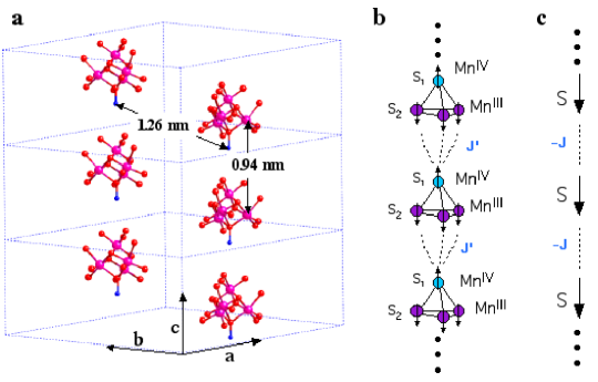
Figure 1: (color online) (a) Unit cells of the Mn₄ crystal. Only the cores of the Mn₄ molecules are shown. The largest spheres are Mn, the smallest Si, and the others O atoms. The distances between next-nearest molecules are indicated. (b) Schematic drawing of the chain-like coupling between the Mn4 SMMs. (c) Scheme of the chain model where the $S=9/2$ spin of each molecule is represented by an arrow.

II Structure of ${\rm Mn}_{4}$ and measuring technique

The studied SMM has the formula [Mn₄O₃(OSiMe₃)(OAc)₃(dbm)₃], called briefly Mn₄. The preparation, X-ray structure, and detailed physical characterization are reported elsewhere Bhaduri03 . Mn₄ crystallizes in a hexagonal space group with crystallographic C₃ symmetry. The unit cell parameters are $a$ = $b$ = 1.998 nm, $c$ = 0.994 nm, $\alpha=\beta=90^{\circ}$, and $\gamma=120^{\circ}$. The unit cell volume is 3.438 nm³ and two molecules are in a unit cell. The complex has a distorted cubane-like core geometry and is Mn${}_{3}^{\rm III}$Mn^IV. The C₃ axis passes through the Mn^IV ion and the triply bridging siloxide group (Fig. 1a). DC and AC magnetic susceptibility measurements indicate a well isolated $S=9/2$ ground state Bhaduri03 .

We found a fine structure of three in the zero-field resonance (Sect. IV.2.1) that is due to the strongest nearest neighbor interactions of about 0.036 T along the $c-$axis of the crystals. This coincides with the shortest Mn–Mn separations of 0.803 nm between two molecules along the $c-$axis, while the shortest Mn–Mn separations perpendicular to the $c-$axis are 1.69 nm and in diagonal direction 1.08 nm (Fig. 1a). We cannot explain the value of 0.036 T by taking into account only dipolar interactions, which should not be larger than about 0.01 T. We believe therefore that small exchange interactions are responsible for the observed value. Indeed, the SMMs are held together by three H bonds C–H–O which are probably responsible for the small exchange interactions.

Fig. 1b shows schematically the antiferromagnetic exchange coupling between the Mn^IV $(S_{1}=3/2)$ ions of one molecule and the Mn^III $(S_{2}=2)$ ion of the neighboring molecule, going via three H bonds C–H–O (not shown in Fig. 1b). This leads to an effective ferromagnetic coupling between the collective spins $(S=9/2)$ of the SMMs (Fig. 1c) because the Mn^IV $(S_{1}=3/2)$ ions and the Mn^III $(S_{2}=2)$ ion in each molecule are antiferromagnetically coupled.

All measurements were performed using an array of micro-SQUIDs WW_ACP01 . The high sensitivity allows us to study single crystals of SMMs of the order of 5 $\mu$m or larger. The field can be applied in any direction by separately driving three orthogonal coils. In the present study, the field was always aligned with the C₃ axis of the molecule, that is the magnetic easy axis, with a precision better than 0.1^∘ WW_PRB04 . The transverse fields were applied transverse to the C₃ axis and along the $a-$axis.

III Spin Hamiltonian and Landau–Zener tunneling

The single spin model (giant spin model) is the simplest model describing the spin system of an isolated SMM. The spin Hamiltonian is

$$\mathcal{H}=-DS_{z}^{2}-BS_{z}^{4}+\mathcal{H}_{{\rm trans}}-g\mu_{\rm B}\mu_{0}\vec{S}\cdot\vec{H}$$ (1)

$S_{x}$, $S_{y}$, and $S_{z}$ are the components of the spin operator, $g~{}\approx~{}2$, $\mu_{\rm B}$ the Bohr magneton; $D$ and $B$ the anisotropy constant defining an Ising type of anisotropy; $\mathcal{H}_{{\rm trans}}$, containing $S_{x}$ or $S_{y}$ spin operators, gives the transverse anisotropy which is small compared to $DS_{z}^{2}$ in SMMs; and the last term describes the Zeeman energy associated with an applied field $\vec{H}$. This Hamiltonian has an energy level spectrum with $(2S+1)$ values which, to a first approximation, can be labeled by the quantum numbers $m=-S,-(S-1),...,S$ taking the $z$-axis as the quantization axis. The energy spectrum can be obtained by using standard diagonalization techniques (Fig. 2). At $\vec{H}=0$, the levels $m=\pm S$ have the lowest energy. When a field $H_{z}$ is applied, the levels with $m>0$ decrease in energy, while those with $m<0$ increase. Therefore, energy levels of positive and negative quantum numbers cross at certain values of $H_{z}$. Although $\mathcal{H}_{\rm trans}$ produces tunneling, it can be neglected when determining the field positions of the level crossing because it is often much smaller than the axial terms. Without $\mathcal{H}_{\rm trans}$ and transverse fields, the Hamiltonian is diagonal and the field position of the crossing of level $m$ with $m^{\prime}$ is given by

$$H_{m,m^{\prime}}=\frac{n\left[D+B\left(m^{2}+m^{\prime 2}\right)\right]}{g\mu_{\rm B}\mu_{0}}$$ (2)

where $n=-(m+m^{\prime})$ is the step index.

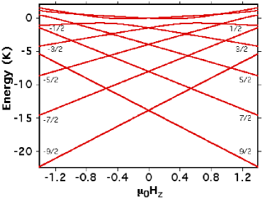
Figure 2: (color online) Zeeman diagram of the 10 levels of the $S=9/2$ manifold of Mn₄ as a function of the field applied along the easy axis. The spin Hamiltonian parameters are $D$ = 0.608 K, $B$ = 3.8 mK, and $E$ = 0.032 K. The levels are approximately labeled with quantum numbers $m=\pm 9/2,\pm 7/2,...,\pm 1/2$.

When the spin Hamiltonian contains transverse terms ($\mathcal{H}_{\rm trans}$), the level crossings can be avoided level crossings. The spin $S$ is in resonance between two states when the local longitudinal field is close to an avoided level crossing. The energy gap, the so-called tunnel splitting $\Delta$, can be tuned by a transverse field (perpendicular to the $S_{z}$ direction) Garg93 ; WW_Science99 ; WW_PRL05 .

The nonadiabatic tunneling probability $P_{m,m^{\prime}}$ between two states when sweeping the longitudinal field $H_{z}$ at a constant rate over an avoided energy level crossing was first discussed by Landau, Zener, and St$\ddot{\rm u}$ckelberg  Landau32 ; Zener32 ; Stuckelberg32 . It is given by

$$P_{m,m^{\prime}}=1-{\rm exp}\left[-\frac{\pi\Delta_{m,m^{\prime}}^{2}}{2\hbar g\mu_{\rm B}|m-m^{\prime}|\mu_{0}dH_{z}/dt}\right]$$ (3)

Here, $m$ and $m^{\prime}$ are the quantum numbers of the avoided level crossing, $dH_{z}/dt$ is the constant field sweeping rates, and $\hbar$ is Planck’s constant.

Fig. 3 presents two different methods to apply the LZ model: in Fig. 3a, the initial state is the lower energy state (standard LZ method) whereas in Fig. 3b it is the higher energy state (inverse LZ method). The tunneling probabilities are given by Eq. 3. In the simple LZ scheme, both methods should lead to the same result. However, when introducing interactions of the spin system with environmental degrees of freedom (phonons, dipolar and exchange interactions, nuclear spins, etc.), both methods are quite different because the final state in Fig. 3a and the initial state in Fig. 3b are unstable. The lifetimes of these states depend on the environmental couplings as well as the level mixing which can be tuned with an applied transverse field. We will see in Sect. III.1 that comparison of the two methods allows the effect of environmental interactions to be observed.

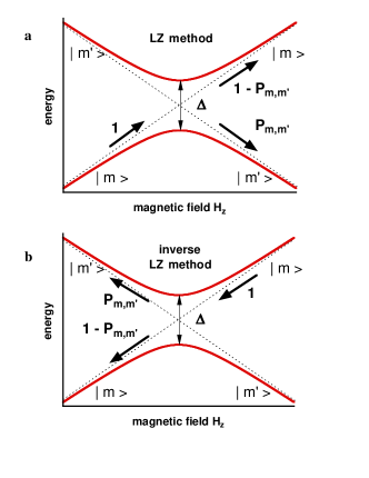
Figure 3: (color online) Detail at a level crossing $m$ with $m^{\prime}$ where the transverse terms (terms containing $S_{x}$ or/and $S_{y}$ spin operators) turn the crossing into an avoided level crossing. The initial state is the lower energy state in (a) (standard LZ method) whereas in (b) it is the higher energy state (inverse LZ method).

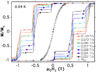
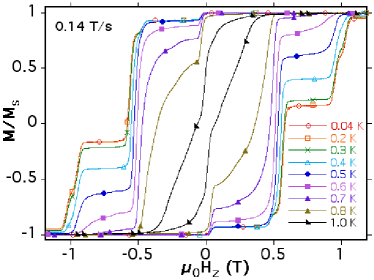
Figure 4: (color online) (a) Hysteresis loop measurements of a single crystal of Mn₄ at low temperatures (40 mK) where thermal activation to excited spin states can be neglected. The field is applied in the direction of the easy axis of magnetization and swept at a constant rate between 0.002 and 0.14 T/s. The dots labeled with $M_{\rm FC}$ are the magnetization after cooling the sample from 5 K down to 0.04 K in a constant applied field $H_{z}$. $M_{\rm FC}$ is used for the equilibrium magnetization $M_{\rm eq}$ in Sect. IV.1. (b) Hysteresis loop measurements similar to Fig. 2 but at different temperatures and for a field sweep rate of 0.14 T/s.

III.1 Landau–Zener tunneling in Mn₄

Landau–Zener tunneling can be seen in hysteresis loop measurements. Figs. 4a and 4b show typical hysteresis loops for a single crystals of Mn₄ at several temperatures and field sweep rates. When the applied field is near an avoided level crossing, the magnetization relaxes faster, yielding steps separated by plateaus. As the temperature is lowered, there is a decrease in the transition rate due to reduced thermally assisted tunneling. A similar behavior was observed in Mn₁₂ acetate clusters Novak95 ; Paulsen95 ; Paulsen95b ; Friedman96 ; Thomas96 and other SMMs Sangregorio97 ; Aubin98 ; Caneschi99 ; Yoo_Jae00 ; Ishikawa05b . The hysteresis loops become temperature-independent below 0.4 K indicating ground state tunneling. The field between two resonances allows us to estimate the anisotropy constants $D$ and $B$. We found:

$$D=g\mu_{\rm B}\mu_{0}\left(H_{z}^{(1)}-\frac{2S^{2}-2S+1}{2S-3}\left(H_{z}^{(1)}-\frac{H_{z}^{(2)}}{2}\right)\right)$$ (4)

$$B=\frac{g\mu_{\rm B}\mu_{0}}{2S-3}\left(H_{z}^{(1)}-\frac{H_{z}^{(2)}}{2}\right)$$ (5)

where $H_{z}^{(1)}$ and $H_{z}^{(2)}$ are the field positions of level crossings $M=-S$ with $S-1$ and $M=-S$ with $S-2$.

The influence of dipolar and intermolecular exchange, which can shift slightly the resonance positions (Sect. IV.2.1), can be avoided by performing minor hysteresis loops involving only few percent of the molecules (Fig. 5). We found the field separations between the zero-field resonance and the first and second resonance are $H_{z}^{(1)}$ = 0.544 T and $H_{z}^{(2)}$ = 1.054 T. Using Egs. 4 and 5, we find $D$ = 0.608 and $B$ = 3.8 mK. These values agree with those obtained from INS and EPR measurements Hill_unpublished .

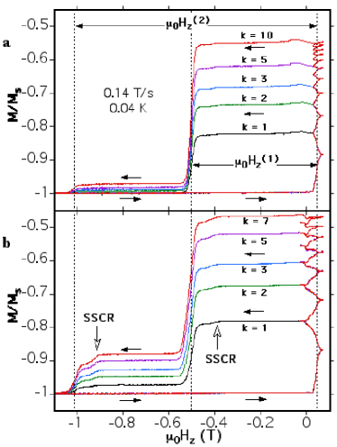
Figure 5: (color online) Minor hysteresis loops of a single crystal of Mn₄. The magnetization was first saturated at -1.4 T. After ramping the field to zero at 0.14 T/s, the field was swept $k$-times back and forth (between 0.028 and 0.07 T in (a) and between -0.028 and 0.07 T in (b)) over the zero-field resonance with a sweep rate of 0.014 T/s. After the $k$-th sweep, the field is quickly swept back to -1.4 T at a rate of 0.14 T/s leading to resonant tunneling at the level crossing $(m,m^{\prime})=(-7/2,9/2)$ and $(-5/2,9/2)$, and allow to determine $\mu_{0}H_{z}^{(1)}$ = 0.544 T and $\mu_{0}H_{z}^{(2)}$ = 1.054 T. The field interval of the $k$ back and forth sweeps corresponds to zero reversed neighbor (0 RN, see Sect. IV.2.1) in (a) whereas it goes over the 0 RN, 1 RN, and 2 RN transitions in (b). Note that the procedure in (a) leads to sharper steps and reduce spin-spin cross-relaxtion (SSCR) (Sect. V) because all reversed spins have two non-reversed neighbors. The transitions of SSCR are indicated in (b).

In order to explain the few minor steps (Fig. 4), not explained with the above Hamiltonion, spin-spin cross-relaxation between adjacent molecules has to be taken into account WW_PRL02 . Such relaxation processes, present in most SMMs, are well resolved for Mn₄ because the spin is small (Sect. V).

The spin-parity effect was established by measuring the tunnel splitting $\Delta$ as a function of transverse field because $\Delta$ is expected to be very sensitive to the spin-parity and the parity of the avoided level crossing. We showed elsewhere that the tunnel splitting increases gradually for an integer spin, whereas it increases rapidly for a half-integer spin WW_PRB02 . In order to apply quantitatively the LZ formula (Eq. 3), we first checked the predicted field sweep rate dependence of the tunneling rate. The SMM crystal was placed in a high negative field to saturate the magnetization, the applied field was swept at a constant rate over one of the resonance transitions, and the fraction of molecules that reversed their spin was measured. The tunnel splitting $\Delta$ was calculated using Eq. 3 and was plotted in Fig. 2 of reference WW_PRB02 as a function of field sweep rate. The LZ method is applicable in the region of high sweep rates where $\Delta_{-9/2,9/2}$ is independent of the field sweep rate. The deviations at lower sweeping rates are mainly due to reshuffling of internal fields WW_PRL99 (Sect. IV.1) as observed for the Fe₈ SMM WW_EPL00 . Such a behavior has recently been simulated Liu01 .

III.1.1 LZ tunneling in the limit of $P_{m,m^{\prime}}<<1$

Fig. 3 of reference WW_PRB02 presents the tunnel splittings obtained by the LZ method as a function of transverse field and shows that the tunnel splitting increases rapidly for a half-integer spin. Figs. 4a and 4b of reference WW_PRB02 present a simulation of the measured tunnel splittings. We found that either the second order term ($E(S_{+}^{2}+S_{-}^{2})$) with $E$ = 0.032 K or a fourth order term ($B_{44}(S_{+}^{4}+S_{-}^{4})$) with $B_{44}$ = 0.03 mK can equally well describe the experimental data. These results suggest that there is a small effect that breaks the C₃ symmetry. This could be a small strain inside the SMM crystal induced by defects, which could result from a loss or disorder of solvent molecules. Recent inelastic neutron scattering measurements confirm the presence of second and fourth order terms Bhaduri03 .

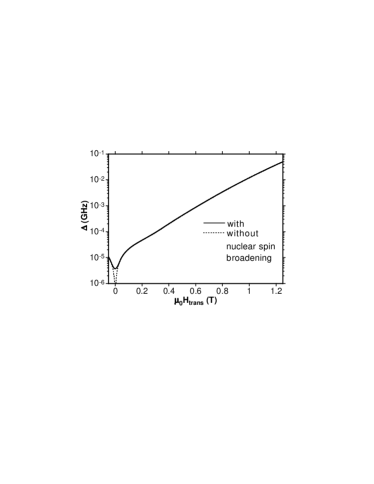
Figure 6: (color online) Calculated tunnel splitting for Mn₄ using $D$ = 0.608 K, $B$ = 3.8 mK, and E = 0.038 K WW_PRB02 . The calculated $\Delta$ has been averaged over all possible orientations of the transverse field in order to represent the arbitrary orientation of the $E$ term. The influence of nuclear spin broadening was taken into account by a Gaussian distribution of transverse field components with a half-width $\sigma=$ 0.035 T.

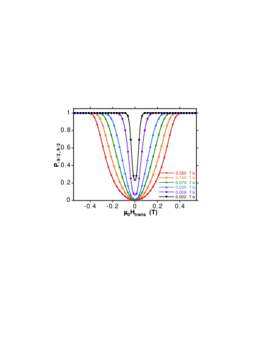
Figure 7: (color online) Calculated LZ tunnel probabilities $P_{\pm 9/2}$ as a function of transverse field using the tunnel splitting from Fig. 6 and the indicated field sweep rates. Only every 100-th calculated point is shown as a symbol.

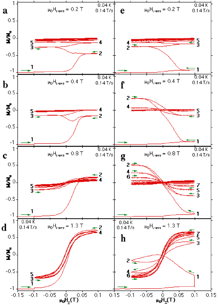
Figure 8: (color online) Magnetization versus applied field scans for (a-d) the LZ method and (e-h) the inverse LZ method. The indicated transverse fields $H_{\rm trans}$ are applied at point 1.

III.1.2 LZ tunneling for large probabilities $P_{m,m^{\prime}}$

Figs. 6 and 7 show respectively the tunnel splitting $\Delta$ and the LZ tunnel probabilities $P_{\pm 9/2}$ as a function of transverse field using the parameters of reference WW_PRB02 (Sect. III.1.1). $P_{\pm 9/2}$ increases rapidly to unity; for example, $P_{\pm 9/2}$ = 1 for $H_{\rm trans}>0.4$ T and field sweep rates $dH/dt$ smaller than 0.28 T/s. The Mn₄ system is therefore ideal to study different regimes of the tunnel probability ranging from kHz to sub-GHz tunnel frequencies (Figs. 6).

Fig. 8 presents the magnetization variation during LZ field sweeps for several transverse fields. The SMM crystal was first placed in a high negative field to saturate the magnetization and the applied field was then swept at a constant rate to the field value of -0.1 or 0.1 T for the LZ (Fig. 8a-d) or inverse LZ method (Fig. 8e-h). At this field value, labeled 1, a transverse field was applied to increase the tunnel probability. Finally, the field is swept back and forth over the zero-field resonance transitions ($m=\pm 9/2$) and the fraction of molecules that reversed their spin was measured.

Note severals points in Fig. 8: (i) in Figs. 8a and 8e, the magnetization increases gradually with each field sweep from $M=-M_{\rm s}$ to $M=0$; (ii) in Fig. 8b, the field sweep from 2 to 3 shows first a decrease and then an increase of magnetization. This is due to next-nearest neighbor effects (Sect. IV.2.1); (iii) in Figs. 8c and 8d, the magnetization increases (decreases) for a positive (negative) field scan. Note that the tunnel probability is 1 for transverse fields larger than 0.3 T (Figs. 7), that is all spins should reverse for each field sweep; (iv) in Figs. 8f and 8g, the magnetization increases much stronger for the field sweep from 1 to 2 than in Figs. 8b and 8c; (v) in Fig. 8h, the field sweep from 1 to 2 shows first an increase and then a decrease of magnetization; (vi) in Figs. 8a to 8c and 8e to 8g, the magnetization tends to relax towards $M$ = 0 whereas in Figs. 8d and 8h, it relaxes towards the field cooled magnetization $M_{\rm FC}$ (Fig. 4a).

The result of a detailed study of the magnetization change $\Delta M$ for LZ field scans like those in Fig. 8 are summarized in Figs. 9 and 10. $\Delta M$ is obtained from $\Delta M=(M_{\rm f}-M_{\rm i})\frac{dH}{dt}/|\frac{dH}{dt}|$ where $M_{\rm i}$ and $M_{\rm f}$ are the initial and final magnetization for a given LZ field sweep. Fig. 10 gives field sweep rate dependence for the field sweep from 1 to 2. These graphs show clearly the crossover between the different regions presented in Fig. 8.

We identify three regions:

(i) at small transverse fields (0 to 0.2 T), that is $P_{\pm 9/2}<<1$, tunneling is dominated by single tunnel transitions and $\Delta M$ follows the LZ formula (Eq. 3). This regime is described in Sect. III.1.1;

(ii) at intermediate transverse fields (0.2 to 0.7 T), that is tunnel probabilities $P_{\pm 9/2}$ between $\approx$0.1 and $\approx$1, $\Delta M$ deviates strongly from Eq. 3 and is governed by reshuffling of internal fields;

(iii) at larger transverse fields, the magnetization reversal starts to be influenced by the direct relaxation process Abragam70 and many-body tunnel events may occur.

The dominating reshuffling of internal fields in region (ii) can be seen when one compares $\Delta M$ in Figs. 8b and 8c for the field sweep from 1 to 2 with those in Figs. 8f and 8g. A backward sweep gives a larger step than a forward sweep. This is expected for a weak ferromagnetically coupled spin chain. Indeed, any spin that reverses shifts (shuffles) its neighboring spins to negative fields. For a forward sweep this means that these spins will not come to resonance whereas in a backwards sweep, these spins might tunnel a little bit late during the field sweep. A more detailed discussion is presented in Sect. IV.2.1

In region (iii) the direct relaxation process Abragam70 between the two lowest levels starts to play a role. This can be seen by the fact that, during the application of the transverse field in point 1 (Figs. 8h), the magnetization starts to relax rapidly. A direct relaxation process is indeed probable when the involved levels start to be mixed by the large transverse field. Because of this level mixing and the intermolecular interactions, multi-tunnel events are possible because neighboring spins start to be entangled.

The inverse LZ method allows us to establish adiabatic LZ transitions. Whereas for the standard LZ method the difference between an adiabatic and strongly decoherent transition is difficult to distinguish, the inverse LZ method allows a clear separation. This is due to the fact that the equilibrium curve and the adiabatic curve are similar for the standard LZ method but not for the inverse LZ method. For example, Fig. 8g shows that there are more than 10 adiabatic LZ passages before the system reaches a disordered state. It is difficult to conclude this from Fig. 8c because strong decoherence would lead to a similar curve.

It is important to note that the transition between regions (ii) and (iii) leads to the shoulder in Fig. 10 which should not be interpreted as quantum phase interference.

Fig. 9 and Fig. 10 are very rich with information and a complete understanding needs a multi-spin simulation.

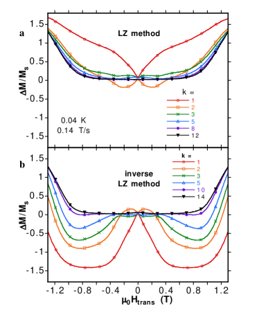
Figure 9: (color online) The change of magnetization $\Delta M=(M_{\rm f}-M_{\rm i})\frac{dH}{dt}/|\frac{dH}{dt}|$ as a function of transverse field $H_{\rm trans}$ for several LZ field sweeps; (a) LZ method and (b) inverse LZ method. Only every 30-th measured point is shown as a symbol.

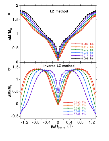
Figure 10: (color online) The change of magnetization $\Delta M=(M_{\rm f}-M_{\rm i})\frac{dH}{dt}/|\frac{dH}{dt}|$ as a function of transverse field $H_{\rm trans}$ for the LZ field sweep from 1 to 2 and for the indicated field sweep rates; (a) LZ method and (b) inverse LZ method.

IV Intermolecular dipolar and exchange interactions

SMMs can be arranged in a crystal with all molecules having the same orientation. Typical distances between molecules are between 1 and 2 nm. Therefore, intermolecular dipole interactions cannot be neglected. An estimation of the dipolar energy can be found in the mean field approximation.

$$E_{\rm dip}=\frac{\mu_{0}}{4\pi}\frac{\left(g\mu_{\rm B}S\right)^{2}}{V}$$ (6)

where $V$ is the volume of the unit cell divided by the number of molecules per unit cell. Typical values of $E_{\rm dip}$ for SMM are between 0.03 and 0.2 K. More precise values, between 0.1 and 0.5 K, were calculated recently Chudnovsky01b ; Fernandez02 .

In addition to dipolar interactions there is also the possibility of a small electronic interaction of adjacent molecules. This leads to very small exchange interactions that depend strongly on the distance and the non-magnetic atoms in the exchange pathway. Until recently, such intermolecular exchange interactions have been assumed to be negligibly small. However, our recent studies on several SMMs suggest that in most SMMs exchange interactions lead to a significant influence on the tunnel process WW_Nature02 ; TironPRB03 ; TironPRL03 ; Hill_Science03 ; Yang03 .

The main difference between dipolar and exchange interactions are: (i) dipolar interactions are long range whereas exchange interactions are usually short range; (ii) exchange interactions can be much stronger than dipolar interactions; (iii) whereas the sign of a dipolar interaction can be determined easily, that of exchange depends strongly on electronic details and is very difficult to predict; and (iv) dipolar interactions depend strongly on the spin ground state $S$, whereas exchange interactions depend strongly on the single-ion spin states. For example, intermolecular dipolar interactions can be neglected for antiferromagnetic SMMs with $S=0$, whereas intermolecular exchange interactions can still be important and act as a source of decoherence.

IV.1 Hole digging method to study intermolecular interactions

Here, we focus on the low temperature and low field limits, where phonon-mediated relaxation is astronomically long and can be neglected. In this limit, the $m~{}=\pm S$ spin states are coupled due to the tunnel splitting $\Delta_{\pm S}$ which is about 10^-7 K for Mn₄ (Sect. III). In order to tunnel between these states, the longitudinal magnetic energy bias $\xi=g\mu_{\rm B}SH_{\rm local}$ due to the local magnetic field $H_{\rm local}$ on a molecule must be smaller than $\Delta_{\pm S}$, implying a local field smaller than $10^{-7}$ T for Mn₄ clusters. Since the typical intermolecular dipole fields for Mn₄ are of the order of 0.01 T and the exchange field between two adjacent molecules of the order of 0.03 T, it seems at first that almost all molecules should be blocked from tunneling by a very large energy bias. Prokof’ev and Stamp have proposed a solution to this dilemma by proposing that fast dynamic nuclear fluctuations broaden the resonance, and the gradual adjustment of the internal fields in the sample caused by the tunneling brings other molecules into resonance and allows continuous relaxation Prokofev98 .

Prokof’ev and Stamp showed that at a given longitudinal applied field $H_{z}$, the magnetization of a crystal of molecular clusters should relax at short times with a square-root time dependence which is due to a gradual modification of the dipole fields in the sample caused by the tunneling

$$M(H_{z},t)=M_{\rm in}+(M_{\rm eq}(H_{z})-M_{\rm in})\sqrt{\Gamma_{\rm sqrt}(H_{z})t}$$ (7)

Here $M_{\rm in}$ is the initial magnetization at time $t$ = 0 (after a rapid field change), and $M_{\rm eq}(H_{z})$ is the equilibrium magnetization at $H_{z}$. Experimentally, $M_{\rm eq}$ is difficult to measure and we replaced it by the field cooled magnetization $M_{\rm FC}(H_{z})$ (Fig. 4a) Intermolecular exchange interactions are neglected in the theory of Prokof’ev and Stamp.

The rate function $\Gamma_{\rm sqrt}(H_{z})$ is proportional to the normalized distribution $P(H_{z})$ of molecules which are in resonance at $H_{z}$

$$\Gamma_{\rm sqrt}(H_{z})=c\frac{\xi_{0}}{E_{D}}\frac{\Delta_{\pm S}^{2}}{4\hbar}P(H_{z})$$ (8)

where $\xi_{0}$ is the line width coming from the nuclear spins, $E_{D}$ is the Gaussian half-width of $P(H_{z})$, and $c$ is a constant of the order of unity which depends on the sample shape. Hence, the measurements of the short time relaxation as a function of the applied field $H_{z}$ give directly the distribution $P(H_{z})$.

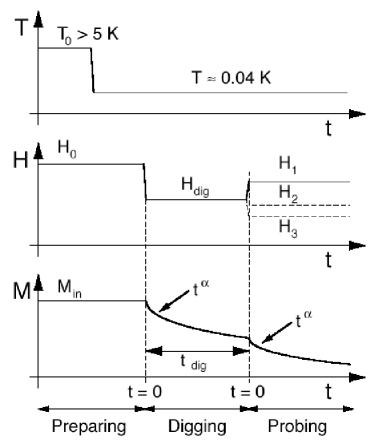
Figure 11: Scheme of the hole digging method presenting the time dependence of temperature, applied field, and magnetization of the sample.

Motivated by the Prokof’ev–Stamp theory Prokofev98 , we developed a new technique—which we called the hole digging method—that can be used to observe the time evolution of molecular states in crystals of nanomagnets WW_PRL99 and to establish resonant tunneling in systems where quantum steps are smeared out by small distributions of molecular environment Soler04 . Here, it has allowed us to measure the statistical distribution of magnetic bias fields in the Mn₄ system that arise from the weak dipole and exchange fields of the clusters. A hole can be “dug” into the distribution by depleting the available spins at a given applied field. Our method is based on the simple idea that after a rapid field change, the resulting short time relaxation of the magnetization is directly related to the number of molecules which are in resonance at the given applied field. Prokof’ev and Stamp have suggested that the short time relaxation should follow a $\sqrt{t}-$relaxation law [equation (7)]. However, the hole digging method should work with any short time relaxation law—for example, a power law

$$M(H_{z},t)=M_{\rm in}+(M_{\rm eq}(H_{z})-M_{\rm in})(\Gamma_{\rm short}(H_{z})t)^{\alpha}$$ (9)

where $\Gamma_{\rm short}$ is a characteristic short time relaxation rate that is directly related to the number of molecules which are in resonance at the applied field $H_{z}$, and $0<\alpha<1$ in most cases. $\alpha$ = 0.5 in the Prokof’ev–Stamp theory [equation (7)] and $\Gamma_{\rm sqrt}$ is directly proportional to $P(H_{z})$ (Eq. 8). The hole digging method can be divided into three steps (Fig. 11):

1. Preparing the initial state. A well-defined initial magnetization state of the crystal of molecular clusters can be achieved by rapidly cooling the sample from high down to low temperatures in a constant applied field $H_{z}^{0}$. For zero applied field ($H_{z}$ = 0) or rather large applied fields ($H_{z}$ $>$ 1 T), one yields the demagnetized or saturated magnetization state of the entire crystal, respectively. One can also quench the sample in a small field of a few milliteslas yielding any possible initial magnetization $M_{\rm in}$. When the quench is fast ($<<$ 1 s), the sample’s magnetization does not have time to relax, either by thermal or by quantum transitions. This procedure yields a frozen thermal equilibrium distribution, whereas for slow cooling rates the molecule spin states in the crystal may tend to a partially ordered ground state. Sect. IV.2.2 shows that, for our fastest cooling rates of $\sim$ 1 s, partial ordering occurs. However, we present a LZ-demagnetization method allowing us to reach a randomly disordered state.

2. Modifying the initial state—hole digging. After preparing the initial state, a field $H_{\rm dig}$ is applied during a time $t_{\rm dig}$, called digging field and digging time, respectively. During the digging time and depending on $H_{\rm dig}$, a fraction of the molecular spins tunnel (back and/or forth); that is, they reverse the direction of magnetization.

3. Probing the final state. Finally, a field $H_{z}^{\rm probe}$ is applied (Fig. 11) to measure the short time relaxation $\Gamma_{\rm short}$ (Eq. 9) which is related to the number of spins that are still free for tunneling after step (2).

The entire procedure is then repeated many times but at other fields $H_{z}^{\rm probe}$ yielding $\Gamma_{\rm short}(H_{z},H_{\rm dig},t_{\rm dig})$ which is related to the distribution of spins $P(H_{z},H_{\rm dig},t_{\rm dig})$ that are still free for tunneling after the hole digging. For $t_{\rm dig}$ = 0, this method maps out the initial distribution.

We applied the hole digging method to several samples of molecular clusters and quantum spin glasses. The most detailed study has been done on the Fe₈ system. We found the predicted $\sqrt{t}$ relaxation (Eq. (7) in experiments on fully saturated Fe₈ crystals Ohm98a ; Ohm98b and on nonsaturated samples WW_PRL99 . These results were in good agreement with simulations Cuccoli99 ; Fernandez01 ; Tupitsyn04 ; Fernandez04 ; Tupitsyn05 ; Tupitsyn05 .

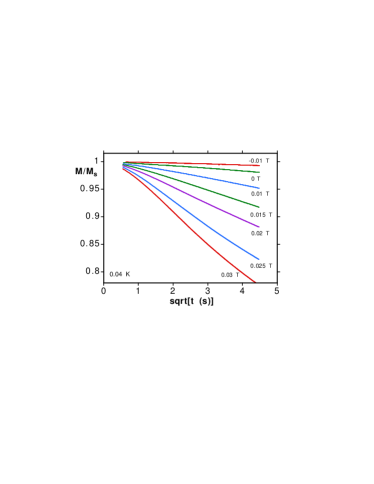
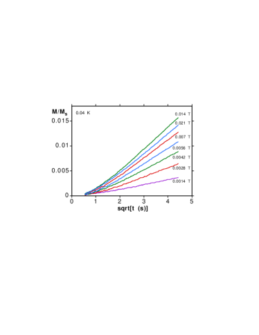
Figure 12: (color online) Typical square root of time relaxation curves for an Mn₄ crystal measured at 40 mK. For each curve, the sample was first (a) saturated or (b) thermally annealed at $H$ = 0. Then the indicated field was applied and the short time relaxation of magnetization was measured. The slope of the lines gives $\Gamma_{\rm sqrt}$ when plotted against the square-root of $t$ as shown.

IV.2 Hole digging applied to Mn₄

Fig. 12 shows typical relaxation curves plotted against the square-root of time. For initially saturated or thermally annealed magnetization, the short time square root law is well obeyed. A fit of the data to Eq. (7) determines $\Gamma_{\rm sqrt}$. We took $M_{\rm eq}=M_{\rm FC}(H_{z})$ of Fig. 4a. A plot of $\Gamma_{\rm sqrt}$ versus $H$ is shown in Fig. 13 for the saturated samples ($M_{\rm in}\approx M_{\rm s}$), as well as for three other values of the initial magnetization which were obtained by quenching the sample from 5 K to 0.04 K in the presence of a small field. The distribution for an initially saturated magnetization is clearly the most narrow reflecting the high degree of order starting from this state. The distributions become broader as the initial magnetization becomes smaller reflecting the random fraction of reversed spins. However, a clear fine structure emerges with bumps at $\pm 0.036$ T and zero field which are due to flipped nearest neighbor spins (Sect. IV.2.1).

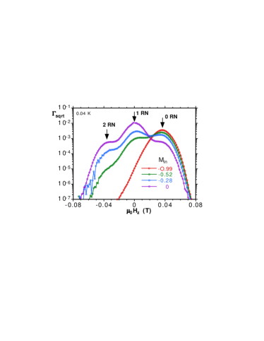
Figure 13: (color online) Field dependence of the short time square-root relaxation rates $\Gamma_{\rm sqrt}(H_{z})$ for three different values of the initial magnetization $M_{\rm in}$. According to equation (8), the curves are proportional to the distribution $P(H_{z})$ of magnetic energy bias due to local internal field distributions in the sample. Note the logarithmic scale for $\Gamma_{\rm sqrt}$. The peaked distribution labeled $M_{\rm in}=-0.99M_{\rm s}$ was obtained by saturating the sample, whereas the other distributions were obtained by thermal annealing. For $M_{\rm in}<<M_{\rm s}$, the curves are distorted by nearest neighbor effects. The peak at $\pm 0.036$ and 0 T are from molecules which have zero, one, or two nearest-neighbors (RN) molecules with reversed magnetization.

Fig. 14(a) shows the short time relaxation rate for a digging field $H_{\rm dig}$ = 0.028 T and for several waiting times. Note the rapid depletion of molecular spin states around $H_{\rm dig}$ and how quickly the same fine-structure, observed in Fig. 13, appears. The hole arises because only spins in resonance can tunnel. The hole is spread out because, as the sample relaxes, the internal fields in the sample change such that spins which were close to the resonance condition may actually be brought into resonance. The overall features are similar to experiments on a fully saturated Fe₈ crystals WW_PRL99 . However, the small chain-like intermolecular interactions make the Mn₄ system unique for a deeper study presented in the following.

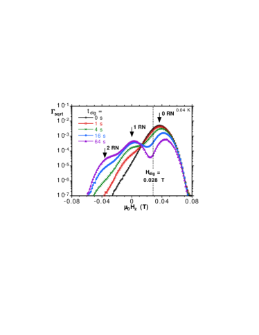
Figure 14: (color online) The field dependence of the short time square root relaxation rates $\Gamma_{\rm sqrt}(H_{z})$ are presented on a logarithmic scale showing the depletion of the molecular spin states by quantum tunneling at $H_{\rm dig}$ = 0.028 T for various digging times $t_{\rm dig}$ and $M_{\rm in}=-M_{s}$.

IV.2.1 Chain-like intermolecular interactions

The Mn₄ molecules are arranged along the $c-$axis in a chain-like structure (Fig. 1). The dipolar coupling between molecules along the chain is significantly larger than between molecules in different chains. In addition there are small exchange coupling between molecules along the chain (Sect. II), leading us to propose the following model.

Each arrow in Fig. 15 represents a molecule. The $+$ and $-$ signs are the magnetic poles. The exchange coupling is represented by $\pm J$. The ground state for a ferromagnetic chain is when all spins are up or down with $+$ and $-$ poles together and $-J$ for all exchange couplings (Fig. 15a). For short, we say that all spins have zero reversed neighbors (2 RN). In order to reverse one spin at its zero-field resonance ($m=-S$ and $m^{\prime}=S$), a magnetic field has to be applied that compensates the interaction field from the neighbors. As soon as one spin is reversed (Fig. 15b), the two neighboring spins see a positive interaction field from one neighbor and a negative one from the other neighbor, that is we say for short that the two spins have one reversed neighbor (1 RN). The interaction field seen by those spins is compensated. Such a spin with 1 RN has a resonance at zero applied field and might reverse creating another spin with 1 RN (Fig. 15c). The third case is when a spin has 2 RN (Fig. 15d). In this case, a negative field has to be applied to compensate the interaction field of the two neighbors.

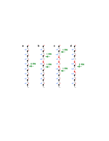
Figure 15: (color online) Schematical representation of a chain of spins with dipole and exchange coupling represented by $+$ and $-$ poles and $\pm J$, respectively. (a) All spins have zero reversed neighbors (0 RN); in (b) and (c), the indicated spins have one reversed neighbor (1 RN), whereas in (d) it has two reversed neighbors (2 RN). The three cases of this two-neighbor-model lead to the fine structure of three for all quantum resonance steps.

In summary, there are three possibilities for a given spin: 0 RN, 1RN, or 2RN with a zero-field resonance shifted to positive (0 RN), zero (1 RN), or negative (2 RN) fields. The influence of the interaction fields of the neighboring molecules is taken into account by a bias field $H_{z}^{\rm bias}$. The effective field $H_{z}$ acting on the molecule is therefore the sum of the applied field $H_{z}^{\rm app}$ and the bias field $H_{z}^{\rm bias}$:

$$H_{z}=H_{z}^{\rm app}+H_{z}^{\rm bias}=H_{z}^{\rm app}+\frac{1}{g\mu_{B}\mu_{0}}\sum_{k=1}^{2}J_{\rm eff}M_{k}$$ (10)

where $M_{k}$ is the quantum number of the neighboring molecule and $J_{\rm eff}$ is an effective exchange coupling taking into account of the nearest neighbor exchange and dipolar coupling. $J_{\rm eff}\approx$ 0.01 K for Mn₄.

Because of the long range character of dipolar fields and the interchain dipolar couplings, the situation in a Mn₄ crystal is more complicated. However, when the exchange interaction is significantly larger than the dipolar interaction, the long range character of the latter leads only to a broadening of the two-neighbor model. Fig. 16 presents schematically the distribution of internal fields of a randomly ordered, a partially ordered, and a completely ordered state with zero total magnetization. Such distributions can be observed with a short-time relaxation, presented in Figs. 13 for a Mn₄ crystal with different initial magnetizations.

We tested the two-neighbor model extensively using, for example, minor hysteresis loops and starting from an initially saturated state (Fig. 15a). When sweeping the field over the zero-field resonance after a negative saturation field, resonant tunneling can only occur at the positive interaction field of 0.036 T. The corresponding step in $M(H)$ indicates that few spins with 0 RN reversed creating spins with 1 RN. This leads to two steps when sweeping the field backwards over the zero-field resonance, one for 0 RN and one for 1 RN (Fig. 5b). When enough spins are reversed, a third step appears at 2 RN.

Similar experiments can be done with the hole digging method (Sect. IV.1). Digging a hole at the field of 0 RN induces a peak at 1 RN (Fig. 14).

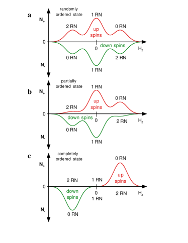
Figure 16: (color online) Schema of the distributions of internal fields of (a) a randomly ordered, (b) a partially ordered, and (c) a completely ordered state with zero total magnetization. Here, $N_{+}$ and $N_{-}$ are the distributions for up and down spins, respectively. The fine structure with three bumps are due to three cases of zero reversed neighbors (0 RN), one reversed neighbor (1 RN), and two reversed neighbors (2 RN).

IV.2.2 Magnetic ordering in crystals of single-molecule magnets

The question of magnetic ordering in molecular magnets has recently been addressed theoretically Chudnovsky01b ; Fernandez02 . Depending on the system ferromagnetic, antiferromagnetic, or spin glass like ground states with ordering temperatures between about 0.2 and 0.5 K have been predicted. Due to the slow relaxation of SMMs at low temperature, ordering might happen at non-accessible long time scales. Recent experimental studies concerned antiferromagnetic ordering in Fe₁₉ SMMs Affronte02 , ferromagnetic ordering of high-spin molecules Morello03 , and partial ordering in the fast tunneling regime of SMMs Evangelisti04 . We present here a simple method to show that partial ordering occurs in crystals of Mn₄ SMMs in the slowly tunneling regime.

The first important step is to create a randomly disordered state (Fig. 16a), that is for any internal field value there are the same number of up and down spins. This means that for any applied field, no magnetization relaxation can be observed because the tunneling from up to down is compensated by tunneling from down to up.

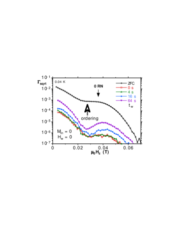
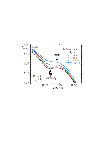
Figure 17: (color online) Short time square root relaxation rate for an Mn₄ crystal measured at 40 mK. (a) The ZFC curve was measured after thermal annealing at $H$ = 0. For the other curves, a randomly disordered state with $M_{\rm in}=0$ was first created by sweeping back and forth the field over the zero-field resonance. After a waiting time $t_{\rm w}$ at $H$ = 0, the short time relaxation rate was measured. The field for one reversed neighbor (1 RN) is indicated. For longer $t_{\rm w}$, $\Gamma_{\rm sqrt}$ approaches the ZFC curve of a partially ordered state. (b) Similar to Fig. 17a but during the waiting time a transverse field of 0.2 T was applied leading to faster ordering.

We tried to achieve a randomly disordered state (Fig. 16a) by a fast quench of the sample temperature from 5 K down to 0.04 K ($\sim$ 1 s). When applying a small field, a $\sqrt{t}$-relaxation is observed (Fig. 12b) showing the the sample was already partially ordered (Fig. 16b).

We found that a randomly disordered state (Fig. 16a) can be achieved by sweeping back and forth the field over the zero-field resonance. During each sweep, few spins tunnel randomly back and fourth. When the Landau–Zener tunnel probability is small ($P_{\rm LZ}<<1$), that is for fast sweep rates of 0.1 T/s for Mn₄, and a large number of back and forth sweeps, a magnetization state can be prepared that shows only a very small relaxation when applying a small field (Fig. 17a). Ordering can then be observed by simply waiting at $H$ = 0 for a waiting time $t_{\rm w}$. The longer is $t_{\rm w}$, the larger is the relaxation, that is the distribution of internal fields evolves from a randomly disordered state (Fig. 16a) to a partially ordered state (Fig. 16b). In order to enhance the ordering, a transverse field can be applied during the waiting time (Fig. 17a). Note that we did not observe complete ordering (Fig. 16c) which is probably due to the entropy, similar to an infinite spin chain which will not order at $T=0$ due to entropy. It is also interesting to note that ordering does not quench tunneling.

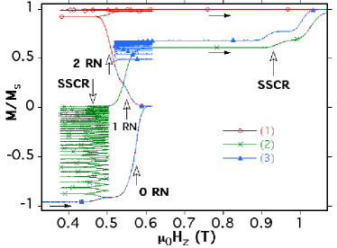
Figure 18: (color online) Minor hysteresis loops of a single crystal of Mn₄. The magnetization was first saturated at -1.4 T. After ramping the field to zero, the field was swept several times back and forth over a part of the tunneling step at the level crossing $(m,m^{\prime})=(-9/2,7/2)$: for curve (1) between 0.38 and 0.62 T; for curve (2) between 0.38 and 0.5 T; for curve (3) between 0.52 and 0.62 T. After the back and forth sweeps, the field is swept to 1.4 T. The field sweep rate for all parts is 0.07 T/s. The fine structure due to nearest neighbor effects and SSCR are indicated.

V Spin-spin cross-relaxation in single-molecule magnets

We showed recently that the one-body tunnel picture of SMMs (Sect. III) is not always sufficient to explain the measured tunnel transitions. An improvement to the picture was proposed by including also two-body tunnel transitions such as spin-spin cross-relaxation (SSCR) which are mediated by dipolar and weak exchange interactions between molecules WW_PRL02 . At certain external fields, SSCRs lead to additional quantum resonances which show up in hysteresis loop measurements as well defined steps. A simple model was used to explain quantitatively all observed transitions. Similar SSCR processes were also observed in the thermally activated regime of a LiYF₄ single crystal doped with Ho ions Giraud01 and for lanthanide SMMs Ishikawa05a .

In order to obtain an approximate understanding of SSCR, we considered a Hamiltonian describing two coupled SMMs which allowed as to explain quantitatively 13 tunnel transitions. We checked also that all 13 transitions are sensitive to an applied transverse field, which always increases the tunnel rate. The parity of the level crossings was also established and in agreement with the two-spin model WW_PRL02 .

It is important to note that in reality a SMM is coupled to many other SMMs which in turn are coupled to many other SMMs. This represents a complicated many-body problem leading to quantum processes involving more than two SMMs. However, the more SMMs that are involved, the lower is the probability for occurrence. In the limit of small exchange couplings and transverse terms, we therefore consider only processes involving one or two SMMs. The mutual couplings between all SMMs should lead mainly to broadenings and small shifts of the observed quantum steps which can be studied with minor hysteresis loops.

Fig. 18 shows typical minor loops at the level crossing $(m,m^{\prime})=(-9/2,7/2)$. In curve (1), the field is swept forth and back over the entire resonance transition. After about two forth and back sweeps, all spins are reversed. Note the next-nearest neighbor fine structure that is in prefect agreement with the two-neighbor model (Sect. IV.2.1). In curve (2), the field is swept forth and back over a SSCR transition (transition 7 in reference  WW_PRL02 ). Note that the relaxation rate is much slower because of the low probability of SSCRs and the fact that this transition is mainly possible for spins with 0 RN or 1 RN. In curve (3), the field is swept forth and back over a part of the level crossing $(m,m^{\prime})=(-9/2,7/2)$ corresponding to spins with 0 RN or 1 RN. In this case, the relaxation rate decreases strongly after the first forth and back sweep because the 2 RN spins cannot tunnel in this field interval.

VI Conclusion

Resonance tunneling measurements on a new high symmetry Mn₄ molecular nanomagnet show levels of detail not yet possible with other SMMs, as a result of higher symmetry and a well isolated spin ground state of $S=9/2$. This has permitted an unprecedented level of analysis of the data to be accomplished, resulting in information not yet attainable with other SMMS. In particular, Landau–Zener (LZ) tunneling in the presence of weak intermolecular dipolar and exchange interactions can be studied, using the LZ and inverse LZ method. The latter has not been applied to any other SMM. Three regions are identified: (i) at small transverse fields, tunneling is dominated by single tunnel transitions; (ii) at intermediate transverse fields, the measured tunnel rates are governed by reshuffling of internal fields, (iii) at larger transverse fields, the magnetization reversal starts to be influenced by the direct relaxation process and many-body tunnel events might occur. The hole digging method is used to study the next-nearest neighbor interactions. At small external fields, it is shown that magnetic ordering occurs which does not quench tunneling. An applied transverse field can increase the ordering rate. Spin-spin cross-relaxations, mediated by dipolar and weak exchange interactions, are proposed to explain additional quantum steps. We would like to emphasize that the present study is mainly experimental, aiming to encourage theorists to develop new tools to model the quantum behavior of weakly interacting quantum spin systems.

References

- (1) L. Landau, Phys. Z. Sowjetunion 2, 46 (1932).
- (2) C. Zener, Proc. R. Soc. London, Ser. A 137, 696 (1932).
- (3) E.C.G. Stckelberg, Helv. Phys. Acta 5, 369 (1932).
- (4) S. Miyashita, J. Phys. Soc. Jpn. 64, 3207 (1995).
- (5) S. Miyashita, J. Phys. Soc. Jpn. 65, 2734 (1996).
- (6) G.Rose and P.C.E. Stamp, Low Temp. Phys. 113, 1153 (1998).
- (7) G.Rose, Ph.D. thesis, The University of British Columbia, Vancouver, 1999.
- (8) M. Thorwart, M. Grifoni, and P. Hnggi, Phys. Rev. Lett. 85, 860 (2000).
- (9) M. N. Leuenberger and D. Loss, Phys. Rev. B 61, 12200 (2000).
- (10) D. A. Garanin and R. Schilling, Phys. Rev. B 66, 174438 (2002).
- (11) D. A. Garanin, Phys. Rev. B 68, 014414 (2003).
- (12) D. A. Garanin and R. Schilling, Phys. Rev. B 71, 184414 (2005).
- (13) R. Sessoli, H.-L. Tsai, A. R. Schake, S. Wang, J. B. Vincent, K. Folting, D. Gatteschi, G. Christou, and D. N. Hendrickson, J. Am. Chem. Soc. 115, 1804 (1993).
- (14) R. Sessoli, D. Gatteschi, A. Caneschi, and M. A. Novak, Nature 365, 141 (1993).
- (15) S. M. J. Aubin, M. W. Wemple, D. M. Adams, H.-L. Tsai, Christou, and D. H. Hendrickson, J. Am. Chem. Soc. 118, 7746 (1996).
- (16) W.Wernsdorfer and R. Sessoli, Science 284, 133 (1999).
- (17) W. Wernsdorfer, N. E. Chakov, and G. Christou, Phys. Rev. Lett. 95, 037203 (2005).
- (18) W. Wernsdorfer, S. Bhaduri, R. Tiron, D. N. Hendrickson, and G. Christou, Phys. Rev. Lett. 89, 197201 (2002).
- (19) W. Wernsdorfer, N. Aliaga-Alcalde, D.N. Hendrickson, and G. Christou, Nature 416, 406 (2002).
- (20) R. Tiron, W. Wernsdorfer, N. Aliaga-Alcalde, and G. Christou, Phys. Rev. B 68, 140407(R) (2003).
- (21) R. Tiron, W. Wernsdorfer, D. Foguet-Albiol, N. Aliaga-Alcalde, and G. Christou, Phys. Rev. Lett. 91, 227203 (2003).
- (22) S.Hill, R.S. Edwards, N.Aliaga-Alcalde, and G.Christou, Science 302, 1015 (2003).
- (23) E. Yang, W. Wernsdorfer, S. Hill, R.S. Edwards, M. Nakano, S. Maccagnano, L.N. Zakharov, A. L. Rheingold, G. Christou, and D.N. Hendrickson, Polyhedron 22, 1727 (2003).
- (24) S. M. J. Aubin, N. R. Dilley, M. B. Wemple, G. Christou, and D. N. Hendrickson, J. Am. Chem. Soc. 120, 4991 (1998).
- (25) S. Bhaduri, M. Pink, K. Folting, W. Wernsdorfer, D.N. Hendrickson, and G. Christou, manuscript in preparation 1, 1 (2003).
- (26) W. Wernsdorfer, Adv. Chem. Phys. 118, 99 (2001).
- (27) W. Wernsdorfer, N. E. Chakov, and G. Christou, Phys. Rev. B 70, 132413 (2004).
- (28) A. Garg, EuroPhys. Lett. 22, 205 (1993).
- (29) M.A. Novak and R. Sessoli, in Quantum Tunneling of Magnetization-QTM’94, Vol. 301 of NATO ASI Series E: Applied Sciences, edited by L. Gunther and B. Barbara (Kluwer Academic Publishers, London, 1995), pp. 171–188.
- (30) C. Paulsen, J.-G. Park, B. Barbara, R. Sessoli, and A. Caneschi, J. Magn. Magn. Mat. 140-144, 379 (1995).
- (31) C. Paulsen and J.-G. Park, in Quantum Tunneling of Magnetization-QTM’94, Vol. 301 of NATO ASI Series E: Applied Sciences, edited by L. Gunther and B. Barbara (Kluwer Academic Publishers, London, 1995), pp. 189–205.
- (32) J. R. Friedman, M. P. Sarachik, J. Tejada, and R. Ziolo, Phys. Rev. Lett. 76, 3830 (1996).
- (33) L. Thomas, F. Lionti, R. Ballou, D. Gatteschi, R. Sessoli, and B. Barbara, Nature (London) 383, 145 (1996).
- (34) C. Sangregorio, T. Ohm, C. Paulsen, R. Sessoli, and D. Gatteschi, Phys. Rev. Lett. 78, 4645 (1997).
- (35) S. M. J. Aubin, N. R. Dilley, M. B. Wemple, G. Christou, and D. N. Hendrickson, J. Am. Chem. Soc. 120, 839 (1998).
- (36) A. Caneschi, D. Gatteschi, C. Sangregorio, R. Sessoli, L. Sorace, A. Cornia, M. A. Novak, C. Paulsen, and W. Wernsdorfer, J. Magn. Magn. Mat. 200, 182 (1999).
- (37) J. Yoo, E. K. Brechin, A. Yamaguchi, M. Nakano, J. C. Huffman, A.L. Maniero, L.-C. Brunel, K. Awaga, H. Ishimoto, G. Christou, and D. N. Hendrickson, Inorg. Chem. 39, 3615 (2000).
- (38) N. Ishikawa, M. Sugita, and W. Wernsdorfer, Angew. Chem. Int. Ed. 44, 2 (2005).
- (39) S. Hill et al., unpublished .
- (40) W. Wernsdorfer, S. Bhaduri, C. Boskovic, G. Christou, and D.N. Hendrickson, Phys. Rev. B 65, 180403(R) (2002).
- (41) W. Wernsdorfer, T. Ohm, C. Sangregorio, R. Sessoli, D. Mailly, and C. Paulsen, Phys. Rev. Lett. 82, 3903 (1999).
- (42) W. Wernsdorfer, A. Caneschi, R. Sessoli, D. Gatteschi, A. Cornia, V. Villar, and C. Paulsen, EuroPhys. Lett. 50, 552 (2000).
- (43) Jie Liu, Biao Wu, Libin Fu, Roberto B. Diener, and Qian Niu, Phys. Rev. B 65, 224401 (2002).
- (44) A. Abragam and B. Bleaney, Electron paramagnetic resonance of transition ions (Clarendon Press, Oxford, 1970).
- (45) X. Mart nez-Hidalgo, E.M. Chudnovsky, and A. Aharony, EuroPhys. Lett. 55, 273 (2001).
- (46) Julio F. Fernandez, Phys. Rev. B 66, 064423 (2002).
- (47) N.V. Prokof’ev and P.C.E. Stamp, Phys. Rev. Lett. 80, 5794 (1998).
- (48) M. Soler, W. Wernsdorfer, K. Folting, M. Pink, and G. Christou, J. Am. Chem. Soc. 126, 2156 (2004).
- (49) T. Ohm, C. Sangregorio, and C. Paulsen, Euro. Phys. J. B 6, 195 (1998).
- (50) T. Ohm, C. Sangregorio, and C. Paulsen, J. Low Temp. Phys. 113, 1141 (1998).
- (51) A. Cuccoli, A. Fort, A. Rettori, E. Adam, and J. Villain, Euro. Phys. J. B 12, 39 (1999).
- (52) J. J. Alonso and J. F. Fernandez, Phys. Rev. Lett. 87, 097205 (2001).
- (53) I. Tupitsyn, P.C.E. Stamp, and N. V. Prokof’ev, Phys. Rev. B 69, 132406 (2004).
- (54) Julio F. Fern ndez and Juan J. Alonso, Phys. Rev. B 69, 024411 (2004).
- (55) I. Tupitsyn, P.C.E. Stamp, and N. V. Prokof’ev, Phys. Rev. B 72, 026402 (2005).
- (56) M. Affronte, J. C. Lasjaunias, W. Wernsdorfer, R. Sessoli, D. Gatteschi, S. L. Heath, A. Fort, and A. Rettori, Phys. Rev. B 66, 064408 (2002).
- (57) A. Morello, F. L. Mettes, F. Luis, J. F. Fern ndez, J. Krzystek, G. Aromi, G. Christou, and L. J. de Jongh, Phys. Rev. Lett. 90, 017206 (2003).
- (58) M. Evangelisti, F. Luis, F. L. Mettes, G. Arom N. Aliaga, J. J. Alonso, G. Christou, and L. J. de Jongh, Phys. Rev. Lett. 93, 117202 (2004).
- (59) R. Giraud, W. Wernsdorfer, A. M. Tkachuk, D. Mailly, and B. Barbara, Phys. Rev. Lett. 87, 057203 (2001).
- (60) N. Ishikawa, M. Sugita, and W. Wernsdorfer, J. Am. Chem. Soc. 127, 3650 (2005).