Breaking of ergodicity and long relaxation times in systems with long-range interactions

Abstract

The thermodynamic and dynamical properties of an Ising model with both short range and long range, mean field like, interactions are studied within the microcanonical ensemble. It is found that the relaxation time of thermodynamically unstable states diverges logarithmically with system size. This is in contrast with the case of short range interactions where this time is finite. Moreover, at sufficiently low energies, gaps in the magnetization interval may develop to which no microscopic configuration corresponds. As a result, in local microcanonical dynamics the system cannot move across the gap, leading to breaking of ergodicity even in finite systems. These are general features of systems with long range interactions and are expected to be valid even when the interaction is slowly decaying with distance.

Systems with long range interactions are rather common in nature LesHouches . In such systems the inter-particle potential decays at large distance $r$ as $1/r^{\alpha}$ with $\alpha\leq d$, in dimension $d$. Examples include magnets with dipolar interactions, wave-particle interactions Barre , gravitational forces Padmanabhan , and Coulomb forces in globally charged systems Nicholson . It is well known that in such systems the various statistical mechanical ensembles need not be equivalent Thirring . For example whereas the canonical ensemble specific heat is always non-negative, it may become negative within the microcanonical ensemble when long range interactions are present Lynden68 . It has recently been suggested that whenever the canonical ensemble exhibits a first order phase transition the canonical and the microcanonical phase diagrams may be different Mukamel01 . This has been demonstrated by a detailed study of a spin-1 Ising model with long range, mean field like, interactions. While the thermodynamic behavior of such models is fairly well understood, their dynamics, and the approach to equilibrium, has not been investigated in detail so far Yama . The aim of the present Letter is to identify some general dynamical features which distinguish systems with long range interactions from those with short range ones.

One characteristic of systems with short range interactions is that the domain in the space of extensive thermodynamic variables $\vec{X}$ over which the model is defined is convex for sufficiently large number of particles. Here the components of the vector $\vec{X}$ are variables like the energy, volume and possibly other extensive parameters corresponding to the system under study. Convexity is a direct result of additivity. By combining two appropriately weighted sub-systems with extensive variables $\vec{X_{1}}$ and $\vec{X_{2}}$, any intermediate value of $\vec{X}$ between $\vec{X_{1}}$ and $\vec{X_{2}}$ may be realized. On the other hand systems with long range interactions are not additive, and thus intermediate values of the extensive variables are not necessarily accessible. This feature has a profound consequence on the dynamics of systems with long range interactions. Gaps may open up in the space of extensive variables and lead to breaking of ergodicity under local microcanonical dynamics of such systems. An example of such gaps in a class of anisotropic $XY$ models has recently been discussed in Celardo .

Another interesting feature of systems with long range interactions is their relaxation time. It is well known that the relaxation time of metastable states grows exponentially with the system size Griffiths . On the other hand the relaxation processes of thermodynamically unstable states are not well understood. In systems with short range interactions the relaxation takes place on a finite time scale. However previous studies of a mean field $XY$ model suggest that this relaxation time diverges with the system size Yama .

In the present Letter we study some of the issues discussed above by considering a spin-$1/2$ Ising model with both long range, mean field like, and short range nearest neighbor interactions on a ring geometry Nagle ; Kardar . We study its thermodynamic and dynamical behavior in both the canonical and microcanonical ensembles. It is found that the two ensembles result in different phase diagrams as was observed in other models Mukamel01 . Moreover, we find that for sufficiently low energy, gaps open up in the magnetization interval $-1\leq m\leq 1$, to which no microscopic configuration corresponds. Thus the phase space breaks into disconnected regions. Within a local microcanonical dynamics the system is trapped in one of these regions, leading to a breakdown of ergodicity even in finite systems. In studying the relaxation time of thermodynamically unstable states, corresponding to local minima of the entropy, we find that unlike the case of short range interactions where this time is finite, here it diverges logarithmically with the system size. We provide a simple explanation for this behavior by analyzing the dynamics of the system in terms of a Langevin equation.

We start by considering an Ising model defined on a ring of $N$ spins $S_{i}=\pm 1$ with long and short range interactions. The Hamiltonian is given by

$${}H=-\frac{K}{2}{\sum_{i=1}^{N}}\left(S_{i}S_{i+1}-1\right)-\frac{J}{2N}\left({\sum_{i=1}^{N}}S_{i}\right)^{2},$$ (1)

where $J>0$ is a ferromagnetic, long range, mean field like coupling, and $K$ is a nearest neighbor coupling which may be of either sign. The canonical phase diagram of this model has been derived in the past Kardar ; Nagle . It has been observed that in the $(K,T)$ plane, where $T$ is the temperature, the model exhibits a phase transition line separating a disordered phase from a ferromagnetic one (see Fig. 1). The transition is continuous for large $K$, where it is given by $\beta=e^{-\beta K}$. Here $\beta=1/T$ and $J=1$ is assumed for simplicity. Throughout this work we take $k_{B}=1$ for the Boltzmann constant. The transition becomes first order below a tricritical point located at an antiferromagnetic coupling $K_{CTP}=-\ln 3/{2\sqrt{3}}\simeq-0.317$.

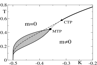
Figure 1: The canonical and microcanonical $(K,T)$ phase diagram. In the canonical ensemble the large $K$ transition is continuous (bold solid line) down to the trictitical point CTP where it becomes first order (dashed line). In the microcanonical ensemble the continuous transition coincides with the canonical one at large $K$ (bold line). It persists at lower K (dotted line) down to the tricritical point MTP where it turns first order, with a branching of the transition line (solid lines). The region between these two lines (shaded area) is not accessible.

We now analyze the model within the microcanonical ensemble. Let $U=-\frac{1}{2}\sum_{i}\left(S_{i}S_{i+1}-1\right)$ be the number of antiferromagnetic bonds in a given configuration characterized by $N_{+}$ up spins and $N_{-}$ down spins. Simple counting yields that the number of microscopic configurations corresponding to $(N_{+},N_{-},U)$ is given, to leading order in $N$, by

$$\Omega(N_{+},N_{-},U)=\left(\begin{array}[]{c}N_{+}\\ U/2\end{array}\right)\left(\begin{array}[]{c}N_{-}\\ U/2\end{array}\right)~{}.\\$$ (2)

Expressing $N_{+}$ and $N_{-}$ in terms of $N$ and the magnetization $M=N_{+}-N_{-}$, and denoting $m=M/N$, $u=U/N$ and the energy per spin $\epsilon=E/N$, one finds that the entropy per spin, $s(\epsilon,m)=\frac{1}{N}\ln\Omega$ is given in the thermodynamic limit by

$${}s(\epsilon,m) = \frac{1}{2}(1+m)\ln(1+m)+\frac{1}{2}(1-m)\ln(1-m)$$ (3)

$$- u\ln u-\frac{1}{2}(1+m-u)\ln(1+m-u)$$

$$- \frac{1}{2}(1-m-u)\ln(1-m-u)~{},$$

where $u$ satisfies

$$\epsilon=-\frac{J}{2}m^{2}+Ku\,.$$ (4)

By maximizing $s(\epsilon,m)$ with respect to $m$ one obtains both the spontaneous magnetization $m_{s}(\epsilon)$ and the entropy $s(\epsilon)\equiv s(\epsilon,m_{s}(\epsilon))$ of the system for a given energy. The temperature, and thus the caloric curve, is given by $1/T=\partial s(\epsilon)/\partial\epsilon$. A straightforward analysis of (3) yields the microcanonical $(K,T)$ phase diagram of the model (Fig. 1), where it is also compared with the canonical one. It is found that the model exhibits a critical line given by the same expression as that of the canonical ensemble. However this line extends beyond the canonical tricritical point, reaching a microcanonical tricritical point at $K_{MTP}\simeq-0.359$, which is computed analytically. For $K<K_{MTP}$ the transition becomes first order and it is characterized by a discontinuity in the temperature. The transition is thus represented by two lines in the $(K,T)$ plane corresponding to the two temperatures at the transition point. These lines are obtained by numerically maximizing the entropy (3).

We now consider the dynamics of the model. This is done by using the microcanonical Monte Carlo dynamics suggested by Creutz Creutz . In this dynamics one samples the microstates of the system with energy $E-E_{D}$ with $E_{D}\geq 0$ by attempting random single spin flips. One can show that, to leading order in the system size, the distribution of the energy $E_{D}$ takes the form

$$P(E_{D})\sim e^{-E_{D}/T}~{}.$$ (5)

Thus, measuring this distribution, yields the temperature $T$ which corresponds to the energy $E$.

In applying this dynamics to our model one should note that to next order in $N$ the energy distribution is given by $P(E_{D})\sim\exp{(-E_{D}/T-E_{D}^{2}/{2C_{V}T^{2}})}$, where $C_{V}=O(N)$ is the specific heat. In extensive systems with short range interactions the specific heat is positive and thus the correction term does not modify the distribution function for large $N$. However in our system $C_{V}$ can be negative in a certain range of $K$ and $E$. It even becomes arbitrarily small near the MTP point, making the next to leading term in the expansion arbitrarily large. This could in principle qualitatively modify the energy distribution. However as long as the entropy is an increasing function of $E$, namely for positive temperatures, the distribution function (5) is valid in the thermodynamic limit. This point is verified by our numerical studies, where an exponential distribution of the energy $E_{D}$ is clearly observed.

We now address the issue of the accessible magnetization intervals in this model. We find that in certain regions in the $(K,E)$ plane, the magnetization $m$ cannot assume any value in the interval $(-1,1)$. There exist gaps in this interval to which no microscopic configuration could be associated. To see this, we take for simplicity the case $N_{+}>N_{-}$. It is evident that the local energy $U$ satisfies $0\leq U\leq 2N_{-}$. The upper bound is achieved in microscopic configurations where all down spins are isolated. This implies that $0\leq u\leq 1-m$. Combining this with (4) one finds that for positive $m$ the accessible states have to satisfy

$$m\leq\sqrt{-2\epsilon}\quad,\quad m\geq m_{+}\quad,\quad m\leq m_{-}$$ (6)

$$\mbox{with}\,\,m_{\pm}=-K\pm\sqrt{K^{2}-2(\epsilon-K)}~{}.$$

Similar restrictions exist for negative $m$. These restrictions yield the accessible magnetization domain shown in Fig. 2 for $K=-0.4$. It is clear that this domain is not convex. Entropy curves $s(m)$ for some typical energies are given in Fig. 3, demonstrating that the number of accessible magnetization intervals changes from one to three, and then to two as the energy is lowered.

This feature of disconnected accessible magnetization intervals, which is typical to systems with long range interactions, has profound implications on the dynamics. In particular, starting from an initial condition which lies within one of these intervals, local dynamics, such as the one applied in this work, is unable to move the system to a different accessible interval. Thus ergodicity is broken in the microcanonical dynamics even at finite $N$.

To demonstrate this point we display in Fig. 4 the time evolution of the magnetization for two cases: one in which there is a single accessible magnetization interval, where one sees that the magnetization switches between the metastable $m=0$ state and the two stable states $m=\pm m_{s}$. In the other case the metastable $m=0$ state is disconnected from the stable ones, making the system unable to switch from one state to the other. Note that this feature is characteristic of the microcanonical dynamics. Using local canonical dynamics, say Metropolis algorithm  Metropolis , would allow the system to cross the forbidden region (by moving to higher energy states where the forbidden region diminishes), and ergodicity is restored in finite systems. However, in the thermodynamic limit, ergodicity would be broken even in the canonical ensemble, as the switching rate between the accessible regions decreases exponentially with $N$.

Figure 2: Accessible region in the $(m,\epsilon)$ plane (shaded area) for $K=-0.4$. For energies in a certain range, gaps in the accessible magnetization values are present.

Figure 3: The $s(m)$ curves for $K=-0.4$, and for typical energy values, demonstrating that gaps in the accessible states develop as the energy is lowered.

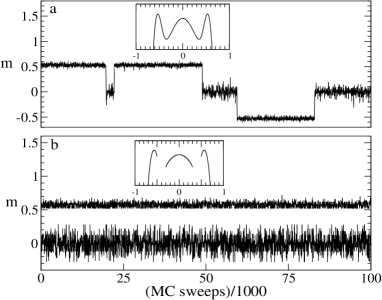
Figure 4: Time evolution of the magnetization for $K=-0.4$ (a) in the ergodic region ($\epsilon=-0.318$) and (b) in the non-ergodic region ($\epsilon=-0.325$). The corresponding entropy curves are shown in the inset.

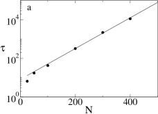
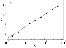
Figure 5: Relaxation time of the $m=0$ state when this state is $(a)$ a local maximum $(K=-0.4,\epsilon=-0.318)$ and $(b)$ a local minimum of the entropy $(K=-0.25,\epsilon=-0.2)$.

We conclude this study by considering the life time $\tau(N)$ of the $m=0$ state, when it is not the equilibrium state of the system. In the case where $m=0$ is a metastable state, corresponding to a local maximum of the entropy (such as in Fig. 4a) we find that the life time satisfies $\tau\sim e^{N\Delta s}$ where $\Delta s$ is the difference in entropy of the $m=0$ state and that of the unstable magnetic state corresponding to the local minimum of the entropy (see Fig. 5a). Such exponential dependence on $N$ has been found in the past in Metropolis type dynamics of the Ising model with mean field interactions Griffiths . Similar behavior has been found in the $XY$ model Torcini and in gravitational systems Chavanis when microcanonical dynamics was applied.

We now turn to the case where the $m=0$ state is thermodynamically unstable, where it corresponds to a local minimum of the entropy. In systems with short range interactions, the relaxation time of this state is finite. Here we find unexpectedly that the life time diverges weakly with $N$, $\tau(N)\sim\log(N)$ (see Fig. 5b). This is to be compared with studies of the life time of the zero magnetization state in the $XY$ model under similar conditions which show that $\tau(N)\sim N^{\alpha}$ with $\alpha\simeq 1.7$ Yama .

In order to understand this behavior we consider the Langevin equation corresponding to the dynamics of the system. The evolution of $m$ is given by

$$\frac{\partial m}{\partial t}=\frac{\partial s}{\partial m}+\xi(t)\,\,\,,\,\,<\xi(t)\xi(t^{\prime})>=D\delta(t-t^{\prime})$$ (7)

where $\xi(t)$ is the usual white noise term. The diffusion constant $D$ scales as $D\sim 1/N$. This can be easily seen by considering the non-interacting case in which the magnetization evolves by pure diffusion where the diffusion constant is known to scale in this form. Taking $s(m)=am^{2}$ with $a>0$, making the $m=0$ state thermodynamically unstable, and neglecting higher order terms, the distribution function of the magnetization, $P(m,t)$, may be calculated. This is done by solving the Fokker-Planck equation corresponding to (7). With the initial condition for the probability distribution $P(m,0)=\delta(m)$, the large time asymptotic distribution is found to be Risken

$$P(m,t)\sim\exp\left[-\frac{ae^{-at}m^{2}}{D}\right]\,.$$ (8)

This is a Gaussian distribution whose width grows with time. The relaxation time corresponds to the width reaching a value of $O(1)$, yielding $\tau\sim-\ln D\sim\ln N$. Similar analysis and simulations can be carried out for the canonical ensemble yielding the same divergence.

In summary, some general features of the dynamical behavior of systems with long range interactions were studied using the microcanonical local dynamics of an Ising model. Properties like gaps in the accessible magnetization interval and breaking of ergodicity in finite systems have been demonstrated. We also find that the relaxation time of an unstable $m=0$ state, corresponding to a local minimum of the entropy, is not finite but rather diverges logarithmically with $N$. We expect these phenomena to appear in other systems with long range interactions which are not necessarily of mean field type. This study is thus of relevance to a wide class of physical systems, such as dipolar systems, self gravitating and Coulomb systems, and interacting wave-particle systems.

We have benefited from discussions with F. Bouchet, A. Campa, T. Dauxois, A. Giansanti, and M. R. Evans. This study was supported by the Israel Science Foundation (ISF), the PRIN03 project Order and chaos in nonlinear extended systems and INFN-Florence . D.M. and S.R. thank ENS-Lyon for hospitality and financial support.

References

- (1) T. Dauxois, S. Ruffo, E. Arimondo, M. Wilkens (Eds.), Dynamics and Thermodynamics of Systems with Long-Range Interactions, Lecture Notes in Physics 602, Springer-Verlag, New York, 2002.
- (2) J. Barré, T. Dauxois, G. De Ninno, D. Fanelli and S. Ruffo, Phys. Rev. E, 69, R045501 (2004).
- (3) T. Padmanabhan, Phys. Rep., 188, 285 (1990).
- (4) D. R. Nicholson, Introduction to Plasma Physics, Krieger Pub. Co. (1992).
- (5) P. Hertel, W. Thirring, Annals of Physics, 63, 520 (1971).
- (6) V. A. Antonov, Leningrad Univ. 7, 135 (1962); Translation in IAU Symposium 113, 525 (1995); D. Lynden-Bell, R. Wood, Monthly Notices of the Royal Astronomical Society, 138, 495 (1968).
- (7) J. Barré, D. Mukamel, S. Ruffo, Phys. Rev. Lett., 87, 030601 (2001).
- (8) Y. Y. Yamaguchi, J Barré, F. Bouchet, T. Dauxois, S. Ruffo, Physica A, 337, 36 (2004).
- (9) F. Borgonovi, G.L. Celardo, M. Maianti and E. Pedersoli, J. Stat. Phys., 116, 1435 (2004).
- (10) R.B. Griffiths, C.Y. Weng and J.S. Langer, Phys. Rev., 149, 1 (1966).
- (11) J. F. Nagle, Phys. Rev. A 2, 2124 (1970); J. C. Bonner and J. F. Nagle, J. Appl. Phys. 42, 1280 (1971).
- (12) M. Kardar, Phys. Rev. B 28, 244 (1983).
- (13) M. Creutz, Phys. Rev. Lett. 50, 1411 (1983)
- (14) N. Metropolis, A.W. Rosenbluth, M. N. Rosenbluth, A. H. Teller and E. Teller, J. Chem. Phys. 21, 1087 (1953).
- (15) M. Antoni, S. Ruffo and A. Torcini, Europhys. Lett., 66, 645 (2004).
- (16) P.H. Chavanis and M. Rieutord, Astronomy and Astrophysics, 412, 1 (2003); P.H. Chavanis, astrph/0404251.
- (17) H. Risken The Fokker-Planck Equation, Springer-Verlag, Berlin (1996), p. 109.