Multi-Photon, Multi-Level Dynamics in a Superconducting Persistent-Current Qubit

Abstract

Single-, two-, and three-photon transitions were driven amongst five quantum states of a niobium persistent-current qubit. A multi-level energy-band diagram was extracted using microwave spectroscopy, and avoided crossings were directly measured between the third and fourth excited states. The energy relaxation times between states connected by single-photon and multi-photon transitions were approximately $30-100$ $\mu s$. Three-photon coherent oscillations were observed between the qubit ground and fourth excited states with a decoherence time of approximately $50$ ns.

Superconducting Josephson junctions are devices that exhibit quantum phenomena amongst their macroscopic degrees of freedom Leggett87a ; Leggett87b . Demonstrations of macroscopic quantum tunneling and energy level quantization provide a basis for utilizing superconducting devices in quantum computing applications Clarke88a . Quantum-state superposition Friedman00a ; Wal00a , multi-qubit spectroscopy Berkley03a ; Xu05a , coherent temporal oscillations Nakamura99a ; Vion02a ; Yu02a ; Martinis02a ; Chiorescu03a and elements of coherent control Pashkin03a ; Yamamoto03a ; Mcdermott05a have been demonstrated with Josephson-based quantum bits Makhlin01a .

Qubit spectroscopy and coherent oscillations can be externally driven in several regimes: by single-photon or multi-photon transitions, with weak or strong driving amplitude, and in two-level or multi-level systems macro_meso_note . Several examples exist of single-photon oscillations in weakly-driven quasi-two-level systems Nakamura99a ; Vion02a ; Yu02a ; Martinis02a ; Chiorescu03a . Nakamura et al. demonstrated single- and multi-photon quantum coherence in a strongly-driven, two-level, charge-qubit system Nakamura . Likewise, Claudon et al. observed single-photon coherent oscillations in a multi-level DC SQUID potential well Claudon04a . Recently, Saito et al. reported single- and multi-photon spectroscopy in a weakly-driven two-level persistent-current (PC) qubit Saito04a . Most demonstrations have utilized aluminum-based devices.

In this paper, we investigate multi-photon, multi-level spectroscopy and dynamics in a weakly-driven niobium persistent-current qubit. We utilize static and time-dependent spectroscopic information from single-, two-, and three-photon transitions to plot a multi-level energy band diagram of the qubit, to identify avoided crossings between its macroscopic states, to measure the energy relaxation time $T_{1}$ from selected excited states, and to demonstrate three-photon coherent oscillations between the qubit’s ground state and fourth excited state.

A PC qubit is a superconducting loop interrupted by three under-damped Josephson tunnel junctions (JTJs) [see Fig. 1(a)]. Two JTJs are designed to have the same critical current $I_{\text{c}}$; the third is $\alpha I_{\text{c}}$. For $0.5<\alpha<1$ and with an externally applied magnetic flux $f_{\text{q}}\approx\Phi_{0}/2$ ($\Phi_{0}\equiv h/2e$ is the flux quantum), the system is analogous to a particle in a two-dimensional double-well potential with a multi-level energy band diagram as simulated (solid lines) in Fig. 2(b). Throughout the paper, the flux will be parameterized by its detuned valued $\delta f_{\text{q}}\equiv f_{\text{q}}-\Phi_{0}/2$. A one-dimensional slice of the double-well potential biased at a flux detuning $\delta f_{\text{q}}\approx 3$ m$\Phi_{0}$ is shown in Fig. 1(b). Energy levels with positive and negative slopes correspond to macroscopic persistent currents $i_{\text{q}}$ of opposing sign, each associated with one of the potential wells Orlando99a . The single-well states are coupled via the potential barrier; the aggregate system has eigenstates with eigenenergies shown in Figs. 1(b) and 2(b). Varying the flux $\delta f_{\text{q}}$ tilts the double-well potential and, thereby, adjusts its eigenstates and energy-levels. Microwaves with frequency matching the energy level spacing can generate transitions between the eigenstates of the undriven system Wal00a ; Chiorescu03a ; Yu02a .

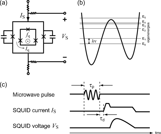
Figure 1: (a) Schematic of the PC qubit surrounded by a readout dc SQUID. “X” denotes a JTJ. The qubit is biased by a magnetic flux $f_{\text{q}}$, and the circulating current of the qubit is $I_{\text{q}}$. (b) Simulated double-well potential of the qubit with eigenenergies $E_{0}-E_{4}$ shown. The energy level separation is $h\nu$. (c) Time sequence of the microwave pulse, SQUID bias current pulse $I_{\text{S}}$, and SQUID voltage response $V_{\text{S}}$ for one measurement trial. The microwave pulse duration is $\tau_{\text{p}}$ and the delay time between microwave pulse off and measurement pulse on is $\tau_{\text{d}}$.

The Nb PC qubits were fabricated with a Nb trilayer process at MIT Lincoln Laboratory Berggren99a . A schematic of the qubit and readout dc SQUID circuit is shown in Fig. 1(a). The inner loop with three JTJs is the PC qubit with a circulating current $I_{\text{p}}\approx 0.45$ $\mu$A and $\alpha\approx 0.84$. The critical current density is $J_{\text{c}}\approx 160$ $\text{A}/\text{cm}^{2}$, $E_{\text{J}}\approx 300$ GHz, and $E_{\text{C}}\approx 0.65$ GHz. The qubit’s loop area is $16\times 16$ $\mu\text{m}^{2}$, with a self-inductance of $L_{\text{q}}\approx 30$ pH. The readout SQUID surrounds the qubit and consists of two JTJs with equal critical current $I_{\text{c0}}=2$ $\mu$A. Both JTJs are shunted with a 1-pF capacitor to lower the SQUID resonant frequency. The SQUID’s loop area is $20\times 20$ $\mu\text{m}^{2}$, with a self-inductance of $L_{\text{SQ}}\approx 60$ pH. The mutual inductance between the qubit and dc SQUID is $M\approx 25$ pH.

Measurements were performed in a dilution refrigerator. The device was magnetically shielded by four cryoperm-10 cylinders and a superconducting can. All electrical leads were carefully attenuated and filtered to minimize noise. For each measurement cycle, we initialized the system by waiting a sufficiently long time, typically 5 ms. Then, as illustrated in Fig. 1(c), a microwave pulse with duration $\tau_{\text{p}}$ is applied to drive quantum-state transitions. After delaying a time interval $\tau_{\text{d}}$, a readout current pulse $I_{\text{S}}$ is sent to the SQUID, and the voltage $V_{\text{S}}$ across the SQUID is monitored with a universal counter. The $I_{\text{S}}$ pulse consists of a 20 ns short pulse, with 5 ns rising and falling edges, and an 18 $\mu$s trailing plateau. The SQUID switches to the finite-voltage state depending on the qubit state and the current $I_{\text{S}}$. This procedure is repeated approximately 1000 times, and the SQUID-switching counts are used to estimate the switching probability $P_{\text{sw}}$. In the following experiments, $P_{\text{sw}}=0$ $(1)$ corresponds to states with positively (negatively) sloped energy bands.

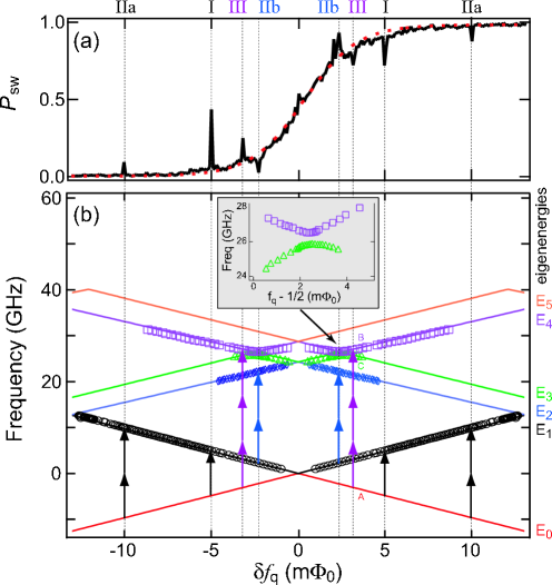
Figure 2: (Color) (a) The switching probability $P_{\text{sw}}$ vs. $\delta f_{\text{q}}$ for a microwave pulse at frequency $\nu=9.9$ GHz with $\tau_{\text{p}}=1$ $\mu$s (solid black line), and thermal distribution in the absence of microwaves (red dashed line). Labels I, IIa, IIb, and III indicate single-, two-, and three-photon resonances. (b) Measured (markers) and fitted (lines) multi-level energy structure of the PC qubit. Eigenenergies $E_{0}\ldots E_{5}$ are shown at right. A, B, and C indicate levels represented by the three-level model (see text). Inset: zoom-in of the avoided crossing between levels $E_{3}$ and $E_{4}$.

Fig. 2(a) shows an example of how $P_{\text{sw}}$ varied as a function of $\delta f_{\text{q}}$ with microwave irradiation at $\nu=9.8$ GHz and of duration $\tau_{\text{p}}=1$ $\mu$s (solid black line). For reference, the expectation value of the qubit initial state in the absence of microwaves is fitted with the thermal distribution function (red dashed line) Orlando99a . In the presence of microwaves, numerous resonances (both peaks and dips) are observed. The resonances are labelled I, IIa, IIb, and III at the top of Fig. 2(a), corresponding to the number of photons involved in each transition. The flux axes in Figs. 2(a) and 2(b) are aligned to coordinate the resonances in the switching probability trace with their corresponding position in the energy band diagram. The experimental data points in Fig. 2(b) are indicated by individual markers, the solid lines are the energy bands obtained from simulating the qubit using the fabrication parameters listed above Orlando99a , and color identifies the first six eigenenergies $E_{0}\ldots E_{5}$. The arrows in Fig. 2(b) are each of height $\nu=9.9$ GHz; the number of stacked arrows corresponds to the number of photons involved in a given transition.

The single-photon resonances, label I in Fig. 2(a), are transitions between the two lowest energy states due to the applied microwave magnetic field at frequency $(E_{1}-E_{0})/h=\nu$. For the same microwave frequency and amplitude, two-photon resonances, label IIa in Fig. 2(a), were also identified between the two lowest energy states at a flux bias yielding $(E_{1}-E_{0})/h=2\nu$. In addition, a 3-photon resonance, label III in Fig. 2(a), was identified between the ground and fourth excited state at a flux bias yielding $(E_{4}-E_{0})/h=3\nu$. Sweeping the microwave frequency varied the flux-distance between resonance pairs with a slope $|\Delta\nu/\Delta f_{\text{q}}|\approx 1/\text{n}\text{ GHz}/\text{m}\Phi_{0}$, allowing us to distinguish $\text{n}=1\ldots 3$ photon transitions and, thereby, reconstruct the energy band diagram. The reconstructed energy band diagram is consistent with that simulated using device fabrication parameters [solid lines, Fig. 2(b)], and it provides clear picture of the multi-level energy-band structure of the qubit.

The additional two-photon resonances, label IIb in Fig. 2(a), are transitions between bands $E_{1}$ and $E_{2}$. A non-zero residual population may exist in $E_{1}$ due to finite temperature, and so the IIb-type transitions were generally observed for flux biases at which $E_{1}$ had non-zero equilibrium population [dashed red line in Fig. 2(a)]. Since $E_{2}$ has the same slope and, thus, circulating current as the ground state energy $E_{0}$ at these flux biases, $P_{\text{sw}}$ decreased (increased) for $\delta f_{\text{q}}<0$ $(\delta f_{\text{q}}>0)$. This is in contrast to transitions I, IIa, and III, for which $P_{\text{sw}}$ increased (decreased), because the accessed bands $E_{1}$ and $E_{4}$ have opposing slope and circulating current to $E_{0}$.

At avoided crossings, the energy bands have zero slope, and the persistent current vanishes. Thus, at $\delta f_{\text{q}}=0$, the SQUID switching-current readout cannot distinguish the $E_{0}$ and $E_{1}$ states. However, we estimated the $E_{0}$ and $E_{1}$ tunnel splitting $\Delta_{12}<0.1$ GHz by fitting to the eigenenergy difference $E_{1}-E_{0}=\sqrt{\Delta_{12}^{2}+\varepsilon^{2}}$, where $\varepsilon$ is the flux-dependent energy difference between the uncoupled states Wal00a . The simulated energy band diagram yielded $\Delta_{12}\sim 10$ MHz. The MHz tunneling splitting indicates that the coupling between the $E_{0}$ and $E_{1}$ states is very weak.

We directly observed an avoided crossing with a tunnel splitting $\Delta_{34}\approx 500$ MHz between energy levels $E_{3}$ and $E_{4}$ using multi-photon transitions [inset Fig. 2(b)], indicating a superposition between two macroscopic quantum states. Although the slopes of $E_{3}$ and $E_{4}$ are zero at the avoided crossing, their SQUID readout signals are distinct from that of the ground state, which has finite slope at this flux bias. By driving transitions from the ground state, we could directly measure the $E_{3}-E_{4}$ avoided crossing and its tunneling splitting $\Delta_{34}$.

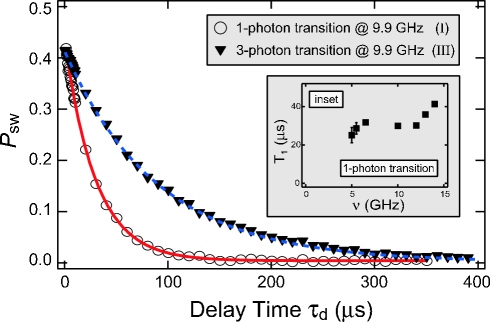
Figure 3: $P_{\text{sw}}$ at $\nu=9.9$ GHz as a function of the readout delay time $\tau_{\text{d}}$. Using a fit exponential decay, we obtained $T_{1}\approx 30\mu$s for the I transition, and $T_{1}\approx 80$ $\mu$s for the III transition in Fig. 2. Inset: $T_{1}$ as a function of $\nu$ for the I transition.

The energy relaxation times $T_{1}$ between macroscopic quantum states were measured by driving population to the excited states ($E_{1}$ and $E_{4}$ in Fig. 2) and monitoring it as a function of $\tau_{\text{d}}$. Fig. 3(a) shows examples of the population decay; an exponential function fits the data remarkably well. The obtained relaxation time from $E_{1}$ is $T_{1}\sim 30$ $\mu$s, and the relaxation time from $E_{4}$ is even longer, $T_{1}\sim 80$ $\mu$s. Both are consistent with the independently measured intra-well relaxation time for a similar qubit design Yu04a ; Segall03a ; Crankshaw03a . We also investigated $T_{1}$ as a function of the energy difference $h\nu$ (inset Fig. 3). The experimental $T_{1}$ tends to increase with increasing $\nu$, qualitatively agreeing with the spin-boson bath model Leggett87a ; Makhlin01a . However, the deviation between the data and theory suggests that we may have other sources and structure to the dissipation. Nevertheless, we can potentially benefit from this long $T_{1}$ in future experiments, such as the three-level flux qubit Zhou02a and superconductive electromagnetic induced transparency Murali04a .

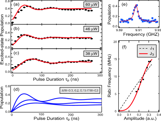
Figure 4: (a)-(c) The amplitude of the 3-photon resonant peaks (III in Fig. 2) vs. the microwave pulse duration $\tau_{\text{p}}$ for $\nu=9.90779$ GHz at different powers. The population oscillations with different frequencies are clearly observed. (d) Coherent oscillations simulated using a three-level model. (e) Lorentzian-fitted (red line) resonance peak data (blue markers) with FWHM $\sim 5$ MHz. The corresponding dephasing time is $\sim 100$ ns. (f) The Rabi frequency as a function of the microwave amplitude. The solid (dashed) line is a best fit to a third-order (first-order) Bessel function of the first kind.

Although the coupling between the ground and first excited states proved too weak to see definitive Rabi oscillations, we were able to observe oscillations in $P_{\text{sw}}$ for transitions between the ground and fourth excited states, since the presence of the avoided crossing (Fig. 2 inset) gives a larger overlap between these states. We biased $\delta f_{\text{q}}$ at the 3-photon resonant peak (III in Fig. 2) and measured the population in the excited state $P_{\text{sw}}$ as a function of microwave pulse duration time $\tau_{\text{p}}$, shown in Fig. 4(a)-(c). The population $P_{\text{sw}}$ oscillates as a function of $\tau_{\text{p}}$, and the oscillation frequency changes with the microwave amplitude. The Rabi decay time is approximately 50 ns, although the oscillation visibilities are only approximately $20\%$. In Fig. 4(f), the oscillation frequencies were plotted as a function of the microwave amplitude. Coherent oscillations were also observed at several frequencies in the range $9<\nu<10$ GHz near the avoided crossing (not shown).

The oscillations in Fig. 4 arise from multi-photon transitions in a multi-level system. We modelled the multi-level, multi-photon transition using a three-level system in which coherent oscillations are driven between levels $A$ and $B$, and level $B$ is taken to be strongly coupled to a third level $C$ [see Fig. 2(b)]. Fig. 4(d) shows coherent oscillations simulated using this model, assuming coupling strengths and decoherence parameters consistent with our qubit. Details of this model will be presented elsewhere, and we only state the qualitative results here: driving levels $A$ and $B$ modifies the coupling between $B$ and $C$, and this modification is dependent upon the driving amplitude. The presence of the third level $C$ results in an amplitude-dependent visibility that vanishes for small driving amplitudes, while, for larger amplitudes, the power-dependent coupling to the third level $C$ effectively detunes the $A$ - $B$ transition. The net result is a limited window of driving amplitudes over which multi-photon transitions can be clearly observed in a multi-level system.

In the limit that the coupling to $C$ is eliminated, the above model reduces to the n-photon, two-level case, in which the Rabi frequency will vary as $J_{\text{n}}(x)$, where $J_{\text{n}}$ is the n-th order Bessel function of the first kind and $x=eV_{\text{ac}}/h\nu$ is proportional to the microwave driving amplitude $V_{\text{ac}}$ Nakamura . The experimental amplitude dependence of the Rabi frequency in Fig. 4(f) is reasonably fit by a third-order Bessel function over the limited range of amplitudes, with the reduced visibilities observed experimentally in Fig. 4(a)-(c) and simulated in Fig. 4(d). Despite the fringe-contrast reduction due to the multiple levels, the $\sim 50$ ns decoherence time of our Nb PC qubit is comparable to those of the qubits fabricated with other superconducting materials Vion02a ; Yu02a ; Martinis02a ; Chiorescu03a .

In summary, we demonstrated multi-level, multi-photon coherent dynamics in a niobium PC qubit. From the single- and multi-photon resonances, we extracted a multi-level energy band diagram. We directly measured an avoided crossing, and we demonstrated three-photon coherent oscillations between the ground and fourth excited state in a multi-level environment.

We gratefully acknowledge E. Macedo, T. Weir, R. Slattery, G. Fitch, and D. Landers for technical assistance with the device fabrication, packaging, and testing at MIT Lincoln Laboratory. We also thank D. Nakada, J Habif, and D. Berns for technical assistance at the MIT campus, and D. Cory and S. Lloyd for helpful discussions. This work was supported by AFOSR (F49620-01-1-0457) under the DURINT program. The work at Lincoln Laboratory was sponsored by the US DoD under Air Force Contract No. F19628-00-C-0002.

References

- (1) A. J. Leggett, S. Chakravarty, A. T. Dorsey, Matthew P. A. Fisher, A. Garg and W. Zwerger, Rev. Mod. Phys. 59, 1 (1987).
- (2) A. J. Leggett, in “Chance and Matter”, Lecture Notes of the Summer School of Theoretical Physics in Les Houches, 1986, Session XLVI, edited by J. Souletie, J. Vannimenus, and R. Stora (North-Holland, Amsterdam, 1987).
- (3) J. Clarke, A. N. Cleland, M. H. Devoret, D. Esteve, and J. M. Martinis, Science 239, 992 (1988).
- (4) J. R. Friedman, V. Patel, W. Chen, S. K. Tolpygo, and J. E. Lukens, Nature 406, 43 (2000).
- (5) C. H. van der Wal, A. C. J. ter Haar, F. K. Wilhelm, R. N. Schouten, C. J. P. M Harmans, T. P. Orlando, S. Lloyd, and J. E. Mooij, Science 290, 773 (2000).
- (6) A. J. Berkley, H. Xu, R. C. Ramos, M. A. Gubrud, F. W. Strauch, P. R. Johnson, J. R. Anderson, A. J. Dragt, C. J. Lobb, and F. C. Wellstood, Science 300, 1548 (2003).
- (7) H. Xu, F. W. Strauch, S. K. Dutta, P. R. Johnson, R. C. Ramos, A. J. Berkley, H. Paik, J. R. Anderson, A. J. Dragt, C. J. Lobb, and F. C. Wellstood, Phys. Rev. Lett. 94, 027003 (2005).
- (8) Y. Nakamura, Y. A. Pashkin, and J. S. Tsai, Nature 398, 786 (1999).
- (9) D. Vion, A. Aassime, A. Cottet, P. Joyez, H. Pothier, C. Urbina, D. Esteve, and M. H. Devoret, Science 296, 886 (2002).
- (10) Y. Yu, S. Han, X. Chu, S. I. Chu, and Z. Wang, Science 296, 889 (2002).
- (11) J. M. Martinis, S. Nam, J. Aumentado, and C. Urbina, Phys. Rev. Lett. 89, 117901 (2002).
- (12) I. Chiorescu, Y. Nakamura, C. J. P. M. Harmans, and J. E. Mooij, Science 299, 1869 (2003).
- (13) We note an additional distinction between superconducting flux and charge qubits made by some authors, e.g., Leggett Leggett87a and Averin Averin99a , with regard to the number of microscopic degrees of freedom involved in the coherent evolution. In flux qubits, this number is macroscopically large, warranting the name “macroscopic coherence.” In charge qubits, in contrast, most of the charge degrees of freedom, except a few, do not participate in the coherent evolution, and thus the aforementioned authors use the “mesoscopic” rather than the “macroscopic” attribution.
- (14) D. V. Averin, Nature 398, 748 (1999).
- (15) Y. A. Pashkin, T. Yamamoto, O. Astafiev, Y. Nakamura, D. V. Averin, and J. S. Tsai, Nature 421, 823 (2003).
- (16) T. Yamamoto, Yu. A. Pashkin, O. Astafiev, Y. Nakamura, and J. S. Tsai, Nature 425, 941 (2003).
- (17) R. McDermott, R. W. Simmonds, M. Steffen, K. B. Cooper, K. Cicak, K. D. Osborn, S. Oh, D. P. Pappas, and J. M. Martinis, Science 307, 1299 (2005).
- (18) Y. Makhlin, G. Schön, and A. Shnirman, Rev. Mod. Phys. 73, 357 (2001).
- (19) Y. Nakamura, Y. A. Pashkin, and J. S. Tsai, Phys. Rev. Lett. 87, 246601 (2001). Y. Nakamura and J. S. Tsai, J. Supercond. 12, 799 (1999).
- (20) J. Claudon, F. Balestro, F. W. J. Hekking, and O. Buisson, Phys. Rev. Lett. 93, 187003 (2004).
- (21) S. Saito, M. Thorwart, H. Tanaka, M. Ueda, H. Nakano, K. Semba, and H. Takayanagi, Phys. Rev. Lett. 93, 037001 (2004).
- (22) T. P. Orlando, J. E. Mooij, L. Tian, C. H. van der Wal, L. Levitov, S. Lloyd, and J. J. Mazo, Phys. Rev. B 60, 15398 (1999).
- (23) K. K. Berggren, E. M. Macedo, D. A. Feld, and J. P. Sage, IEEE Trans. Appl. Supercond. 9, 3271 (1999).
- (24) Y. Yu, D. Nakada, J. C. Lee, B. Singh, D. S. Crankshaw, T. P. Orlando, K. K. Berggren, and W. D. Oliver, Phys. Rev. Lett. 92, 117904 (2004).
- (25) K. Segall, D. Crankshaw, D. Nakada, T. P. Orlando, L. S. Levitov, S. Lloyd, N. Markovic, S. O. Valenzuela, M. Tinkham, K. K. Berggren, Phys. Rev. B 67, 220506(R) (2003).
- (26) D. S. Crankshaw, K. Segall, D. Nakada, T. P. Orlando, L. S. Levitov, S. Lloyd, S. O. Valenzuela, N. Markovic, M. Tinkham and K. K. Berggren, Phys. Rev. B 69, 144518 (2004).
- (27) Z. Zhou, Shih-I Chu, and S. Han, Phys. Rev. B 66, 054527 (2002).
- (28) K. V. R. M. Murali, Z. Dutton, W. D. Oliver, D. S. Crankshaw, and T. P. Orlando, Phys. Rev. Lett. 93, 087003 (2004).