Pseudogaps in Strongly Correlated Metals: A generalized dynamical mean-field theory approach

Abstract

We generalize the dynamical–mean field (DMFT) approximation by including into the DMFT equations some length scale $\xi$ via a momentum dependent “external” self–energy $\Sigma_{\bf k}$. This external self–energy describes non-local dynamical correlations induced by short–ranged collective SDW–like antiferromagnetic spin (or CDW–like charge) fluctuations. At high enough temperatures these fluctuations can be viewed as a quenched Gaussian random field with finite correlation length. This generalized DMFT+$\Sigma_{\bf k}$ approach is used for the numerical solution of the weakly doped one–band Hubbard model with repulsive Coulomb interaction on a square lattice with nearest and next nearest neighbour hopping. The effective single impurity problem in this generalized DMFT+$\Sigma_{\bf k}$ is solved by numerical renormalization group (NRG). Both types of strongly correlated metals, namely (i) doped Mott insulator and (ii) the case of bandwidth $W\lesssim U$ ($U$ — value of local Coulomb interaction) are considered. Densities of states, spectral functions and ARPES spectra calculated within DMFT+$\Sigma_{\bf k}$ show a pseudogap formation near the Fermi level of the quasiparticle band.

I Introduction

Among the numerous anomalies of the normal phase of high–temperature superconductors the observation of a pseudogap in the electronic spectrum of underdoped copper oxides Tim ; MS is especially interesting. Despite continuing discussions on the nature of the pseudogap, the preferable “scenario” for its formation is most likely based on the model of strong scattering of the charge carriers by short–ranged antiferromagnetic (AFM, SDW) spin fluctuations MS ; Pines . In momentum representation this scattering transfers momenta of the order of ${\bf Q}=(\frac{\pi}{a},\frac{\pi}{a})$ ($a$ — lattice constant of two dimensional lattice). This leads to the formation of structures in the one-particle spectrum, which are precursors of the changes in the spectra due to long–range AFM order (period doubling). As a result we obtain non–Fermi liquid like behaviour (dielectrization) of the spectral density in the vicinity of the so called “hot-spots” on the Fermi surface, appearing at intersections of the Fermi surface with antiferromagnetic Brillouin zone boundary (umklapp surface) MS .

Within this spin–fluctuation scenario a simplified model of the pseudogap state was studied MS ; Sch ; KS under the assumption that the scattering by dynamic spin fluctuations can be reduced for high enough temperatures to a static Gaussian random field (quenched disorder) of pseudogap fluctuations. These fluctuations are defined by a characteristic scattering vector from the vicinity of ${\bf Q}$, with a width determined by the inverse correlation length of short–range order $\kappa=\xi^{-1}$, and by appropriate energy scale $\Delta$ (typically of the order of crossover temperature $T^{*}$ to the pseudogap state MS ).

Undoped cuprates are antiferromagnetic Mott insulators with $U\gg W$ ($U$ — value of local Coulomb interaction, $W$ — bandwidth of non–interacting band), so that correlation effects are very important. It is thus clear that the electronic properties of underdoped (and probably also optimally doped) cuprates are governed by strong electronic correlations too, so that these systems are typical strongly correlated metals. Two types of correlated metals can be distinguished: (i) the doped Mott insulator and (ii) the bandwidth controlled correlated metal $W\approx U$. Both types will be considered in this paper.

A state of the art tool to describe such correlated systems is the dynamical mean–field theory (DMFT) MetzVoll89 ; vollha93 ; pruschke ; georges96 ; PT . The characteristic features of correlated systems within the DMFT are the formation of incoherent structures, the so-called Hubbard bands, split by the Coulomb interaction $U$, and a quasiparticle (conduction) band near the Fermi level dynamically generated by the local correlations MetzVoll89 ; vollha93 ; pruschke ; georges96 ; PT .

Unfortunately, the DMFT is not useful to the study the “antiferromagnetic” scenario of pseudogap formation in strongly correlated metals. This is due to the basic approximation of the DMFT, which amounts to the complete neglect of non-local dynamical correlation effects.

Besides the extended DMFT Si96 , which locally includes coupling to nonlocal dynamical fluctuations, a straightforward way to extend the DMFT are the so-called cluster mean-field theories TMrmp . Two variants of this approach are the dynamical cluster approximation (DCA)TMrmp and cellular DMFT (CDMFT)KSPB . In particular the DCA has been applied to study the low-energy properties of the Hubbard model, systematically including short- to medium ranged nonlocal correlations. Both improve on the cluster perturbation theory (CPT) Gross94 ; Senechal00 , a first attempts to use finite-size calculations to obtain approximate results for the thermodynamic limit.

However, these approaches have certain drawbacks from both technical and interpretation points of view. First, the effective quantum single impurity problem becomes rather complex. Thus, most computational methods available for the DMFT can be applied for the smallest clusters only TMrmp ; Kyung05 ; CivKot , i.e. include nearest-neighbor fluctuations only. For medium- to long-ranged correlations one is currently restricted to Quantum Monte-CarloQMC . Since for cluster problems again a sign problem arises, one is restricted to relatively small values of the local Coulomb interaction and high temperatures. Second, the interpretation of electronic structures found has to be based on reliable input from other, typically approximate, complementary techniques.

The aim of the present paper is to propose such a novel approach, which on the one hand retains the single-impurity description of the DMFT, viz a proper account for local correlations and the possibility to use very efficient impurity solvers like NRGNRG ; BPH ; on the other hand, we include non-local correlations on a non-perturbative model basis, which allows to control characteristic scales and also types of non-local fluctuations. This latter point allows for a systematical study of the influence of non-local fluctuations on the electronic properties and in particular provide valuable hints on physical origin and possible interpretation of results found in e.g. more refined theoretical approaches.

The paper is organized as follows: In section II we present a derivation of the self–consistent generalization we call DMFT+$\Sigma_{\bf k}$ which includes short-ranged dynamical correlations to some extent. Section III describes the construction of the k–dependent self–energy, and some computational details are presented in section IV.1. Results and a discussion are given in the sections IV. Then the paper is ended with summary section V together with overview of related recent approaches and results on pseudogap issue.

II Introducing length scale into DMFT: DMFT+$\Sigma_{\bf k}$ approach

The basic shortcoming of the traditional DMFT approach MetzVoll89 ; vollha93 ; pruschke ; georges96 ; PT is the neglect of momentum dependence of the electron self–energy. This approximation in principle allows for an exact solution of correlated electron systems fully preserving the local part of the dynamics introduced by electronic correlations. To include non–local effects, while remaining within the usual “single impurity analogy”, we propose the following procedure. To be definite, let us consider a standard one-band Hubbard model from now on. The extension to multi-orbital or multi-band models is straightforward. The major assumption of our approach is that the lattice and Matsubara “time” Fourier transformed of the single-particle Green function can be written as:

$$G_{\bf k}(i\omega)=\frac{1}{i\omega+\mu-\varepsilon({\bf k})-\Sigma(i\omega)-\Sigma_{\bf k}(i\omega)},\qquad\omega=\pi T(2n+1),$$ (1)

where $\Sigma(i\omega)$ is the local contribution to self–energy, surviving in the DMFT, while $\Sigma_{\bf k}(i\omega)$ is some momentum dependent part. We suppose that this last contribution is due to either electron interactions with some “additional” collective modes or order parameter fluctuations, or may be due to similar non–local contributions within the Hubbard model itself.

To avoid possible confusion we must stress that $\Sigma_{\bf k}(i\omega)$ can in principle also contain local (momentum independent) contributions, which obviously vanish in the limit of infinite dimensionality $d\to\infty$ and are not taken into account within DMFT. Due to this fact there is no double counting of diagrams within our approach to the Hubbard model. This question does not arise at all if we consider $\Sigma_{\bf k}(i\omega)$ appearing due to some “additional” interaction. More important is that the assumed additive form of the self–energy $\Sigma(i\omega)+\Sigma_{\bf k}(i\omega)$ implicitly corresponds to neglect of possible interference of these local (DMFT) and non–local contributions. Furthermore, both contributions to the total self-energy $\Sigma(i\omega)+\Sigma_{\bf k}(i\omega)$ individually obeye causality by construction. Thus, the sum and finally the propagator (1) constructed from it are causal, too.

The self–consistency equations of our generalized DMFT+$\Sigma_{\bf k}$ approach are formulated as follows:

1. Start with some initial guess of local self–energy $\Sigma(i\omega)$, e.g. $\Sigma(i\omega)=0$.

2. Construct $\Sigma_{\bf k}(i\omega)$ within some (approximate) scheme, taking into account interactions with collective modes or order parameter fluctuations which in general can depend on $\Sigma(i\omega)$ and $\mu$.

3. Calculate the local Green function

   $$G_{ii}(i\omega)=\frac{1}{N}\sum_{\bf k}\frac{1}{i\omega+\mu-\varepsilon({\bf k})-\Sigma(i\omega)-\Sigma_{\bf k}(i\omega)}.$$ (2)

4. Define the “Weiss field”

   $${\cal G}^{-1}_{0}(i\omega)=\Sigma(i\omega)+G^{-1}_{ii}(i\omega).$$ (3)

5. Using some “impurity solver” to calculate the single-particle Green function for the effective single Anderson impurity problem, defined by Grassmanian integral

   $$G_{d}(\tau-\tau^{\prime})=\frac{1}{Z_{\text{eff}}}\int Dc^{+}_{i\sigma}Dc_{i\sigma}c_{i\sigma}(\tau)c^{+}_{i\sigma}(\tau^{\prime})\exp(-S_{\text{eff}})$$ (4)

   with effective action for a fixed site (“single impurity”) $i$

   $$S_{\text{eff}}=-\int_{0}^{\beta}d\tau_{1}\int_{0}^{\beta}d\tau_{2}c_{i\sigma}(\tau_{1}){\cal G}^{-1}_{0}(\tau_{1}-\tau_{2})c^{+}_{i\sigma}(\tau_{2})+\int_{0}^{\beta}d\tau Un_{i\uparrow}(\tau)n_{i\downarrow}(\tau)\;\;,$$ (5)

   $Z_{\text{eff}}=\int Dc^{+}_{i\sigma}Dc_{i\sigma}\exp(-S_{\text{eff}})$, and $\beta=T^{-1}$. This step produces a new set of values $G^{-1}_{d}(i\omega)$.

6. Define a new local self–energy

   $$\Sigma(i\omega)={\cal G}^{-1}_{0}(i\omega)-G^{-1}_{d}(i\omega).$$ (6)

7. Using this self–energy as “initial” one in step 1, continue the procedure until (and if) convergency is reached to obtain

   $$G_{ii}(i\omega)=G_{d}(i\omega).$$ (7)

Eventually, we get the desired Green function in the form of (1), where $\Sigma(i\omega)$ and $\Sigma_{\bf k}(i\omega)$ are those appearing at the end of our iteration procedure. A more detailed derivation of this scheme within a diagrammatic approach is given in the Appendix A.

III Construction of k–dependent self–energy

For the momentum dependent part of the single-particle self–energy we concentrate on the effects of scattering of electrons from collective short-range SDW–like antiferromagnetic spin (or CDW–like charge) fluctuations. To calculate $\Sigma_{\bf k}(i\omega)$ for an electron moving in the quenched random field of (static) Gaussian spin (or charge) fluctuations with dominant scattering momentum transfers from the vicinity of some characteristic vector ${\bf Q}$ (“hot-spots” model MS ), we use a slightly generalized version of the recursion procedure proposed in Refs. Sch ; KS ; MS79 which takes into account all Feynman diagrams describing the scattering of electrons by this random field. This becomes possible due to a remarkable property of our simplified version of “hot-spots” model that under certain conditions the contribution of an arbitrary diagram with intersecting interaction lines is actually equal to the contribution of some diagram of the same order without intersections of these lines KS ; MS79 . Thus, in fact we can limit ourselves to consideration of only diagrams without intersecting interaction lines, taking the contribution of diagrams with intersections into account with the help of additional combinatorial factors, which are attributed to “initial” vertices or just interaction lines MS79 . As a result we obtain the following recursion relation (continuous fraction representation MS79 ):

$$\Sigma_{n}(i\omega{\bf k})=\Delta^{2}\frac{s(n)}{i\omega+\mu-\Sigma(i\omega)-\varepsilon_{n}({\bf k})+inv_{n}\kappa-\Sigma_{n+1}(i\omega,{\bf k})}\;\;.$$ (8)

Term $\Sigma_{n}(i\omega,{\bf k})$ of recurring sequence contains all contributions of diagrams with the number of interaction lines $\geq n$. Then

$$\Sigma_{\bf k}(i\omega)=\Sigma_{n=1}(i\omega,{\bf k})$$ (9)

is the sum of all diagrammatic contributions up to $2n$-th order. Since the convergence of this recursion procedure for $\Sigma_{n}(i\omega,{\bf k})$ is rather fast, one can take contribution for large enough n equal to zero and doing recursion backwards to $n=1$ get desired physical self–energy KS .

The quantity $\Delta$ characterizes the energy scale and $\kappa=\xi^{-1}$ is the inverse correlation length of short–range SDW (CDW) fluctuations, $\varepsilon_{n}({\bf k})=\varepsilon({\bf k+Q})$ and $v_{n}=|v_{\bf k+Q}^{x}|+|v_{\bf k+Q}^{y}|$ for odd $n$ while $\varepsilon_{n}({\bf k})=\varepsilon({\bf k})$ and $v_{n}=|v_{\bf k}^{x}|+|v_{\bf k}^{y}|$ for even $n$. The velocity projections $v_{\bf k}^{x}$ and $v_{\bf k}^{y}$ are determined by usual momentum derivatives of the “bare” electronic energy dispersion $\varepsilon({\bf k})$. Finally, $s(n)$ represents a combinatorial factor with

$$s(n)=n$$ (10)

for the case of commensurate charge (CDW-type) fluctuations with ${\bf Q}=(\pi/a,\pi/a)$ MS79 . For incommensurate CDW fluctuationsMS79 (when ${\bf Q}$ is not “locked” to the period of inverse lattice) one finds

$$s(n)=\left\{\begin{array}[]{cc}\frac{n+1}{2}&\mbox{for odd $n$}\\ \frac{n}{2}&\mbox{for even $n$}.\end{array}\right.$$ (11)

If we want to take into account the (Heisenberg) spin structure of interaction with spin fluctuations in “nearly antiferromagnetic Fermi–liquid” (spin–fermion (SF) model of Ref. Sch , SDW-type fluctuations), the combinatorics of diagrams becomes more complicated. Spin–conserving scattering processes obey commensurate combinatorics, while spin–flip scattering is described by diagrams of incommensurate type (“charged” random field in terms of Ref. Sch ). In this model the recursion relation for the single-particle Green function is again given by (8), but the combinatorial factor $s(n)$ now acquires the following form Sch :

$$s(n)=\left\{\begin{array}[]{cc}\frac{n+2}{3}&\mbox{for odd $n$}\\ \frac{n}{3}&\mbox{for even $n$}.\end{array}\right.$$ (12)

Obviously, with this procedure we introduce an important length scale $\xi$ not present in standard DMFT. Physically this scale mimics the effect of short–range (SDW or CDW) correlations within fermionic “bath” surrounding the effective single Anderson impurity of the DMFT. We expect that such a length-scale will lead to a competition between local and non-local physics.

An important aspect of the theory is that both parameters $\Delta$ and $\xi$ can in principle be calculated from the microscopic model at hand. For example, using the two–particle selfconsistent approach of Ref. VT with the approximations introduced in Refs. Sch ; KS , one can derive within the standard Hubbard model the following microscopic expression for $\Delta$:

$$\Delta^{2}=\frac{1}{4}U^{2}\frac{<n_{i\uparrow}n_{i\downarrow}>}{<n_{i\uparrow}><n_{i\downarrow}>}[<n_{i\uparrow}>+<n_{i\downarrow}>-2<n_{i\uparrow}n_{i\downarrow}>]=$$

$$=U^{2}\frac{<n_{i\uparrow}n_{i\downarrow}>}{n^{2}}<(n_{i\uparrow}-n_{i\downarrow})^{2}>=$$

$$=U^{2}\frac{<n_{i\uparrow}n_{i\downarrow}>}{n^{2}}\frac{1}{3}<{\vec{S}}_{i}^{2}>,$$ (13)

where we consider only scattering from antiferromagnetic spin fluctuations. The different local quantities – spin fluctuation $<{\vec{S}}_{i}^{2}>$, density $n$ and double occupancy $<n_{i\uparrow}n_{i\downarrow}>$ – can easily be calculated within the standard DMFT georges96 . A detailed derivation of (13) and computational results for $\Delta$ obtained by DMFT using quantum Monte–Carlo (QMC) to solve the effective single impurity problem are presented in Appendix B. A corresponding microscopic expressions for the correlation length $\xi$ can also be derived within the two–particle self–consistent approach VT . However, we expect those results for $\xi$ to be less reliable, because this approach is valid only for relatively small (or medium) values of $U/t$. Thus, in the following we will consider both $\Delta$ and especially $\xi$ as some phenomenological parameters to be determined from experiments.

IV Results and discussion

IV.1 Computation details

In the following, we want to discuss results for a standard one-band Hubbard model on a square lattice. With nearest ($t$) and next nearest ($t^{\prime}$) neighbour hopping integrals the dispersion then reads

$$\varepsilon({\bf k})=-2t(\cos k_{x}a+\cos k_{y}a)-4t^{\prime}\cos k_{x}a\cos k_{y}a\;\;,$$ (14)

where $a$ is the lattice constant. The correlations are introduced by a repulsive local two-particle interaction $U$. We choose as energy scale the nearest neighbour hopping integral $t$ and as length scale the lattice constant $a$.

For a square lattice the bare bandwidth is $W=8t$. To study a strongly correlated metallic state obtained as doped Mott insulator we use $U=40t$ as value for the Coulomb interaction and a filling $n=0.8$ (hole doping). The particular choice of the latter value for $U$ is motivated by two aspects. First, this value of $U$ leads to an insulating DMFT+$\Sigma_{\bf k}$ solution at half-filling. Second, estimations of $U$ for stoichiometric La₂CuO₄ (high-T_C prototype compound) based on constrained LDAGunnarsson89 calculations typically give $U$ of the order of 10 eVLSCO_U_value , which corresponds to 40t to our choice of parameters. The correlated metal in the case of $W\gtrsim U$ is realized via $U=4t$ – a value used in various theoretical papers discussing the pseudogap state – and two fillings: half-filling ($n=1.0$) and $n=0.8$ (hole doping). As typical values for $\Delta$ we choose $\Delta=t$ and $\Delta=2t$ (actually as approximate limiting values — cf. Appendix B) and for the correlation length $\xi=2a$ and $\xi=10a$ (motivated mainly by experimental data for cuprates MS ; Sch ).

The DMFT maps the lattice problem onto an effective, self–consistent single impurity defined by Eqs. (4)-(5). In our work we employ as “impurity solvers” two reliable numerically exact methods — quantum Monte–Carlo (QMC) QMC and numerical renormalization group (NRG) NRG ; BPH . Calculations were done for the case $t^{\prime}=0$ and $t^{\prime}/t$=-0.4 (more or less typical for cuprates) at two different temperatures $T=0.088t$ and $T=0.356t$ (for NRG computations) . QMC computations of double occupancies as functions of filling were done at temperatures $T=0.1t$ and $T=0.4t$  .

Below we present results only for most typical dependences and parameters, more data and figures can be found in Ref. cm05 .

IV.2 Generalized DMFT+$\Sigma_{\bf k}$ approach: densities of states

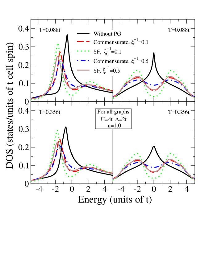
Figure 1: (Color online) Comparison of DOS obtained from DMFT(NRG)+$\Sigma_{\bf k}$ calculations for different combinatorical factors (SF — spin–fermion model, commensurate), inverse correlation lengths ($\xi^{-1}$) in units of the lattice constant, temperatures ($T$) and the value of pseudogap potential $\Delta=2t$. Left column corresponds to $t^{\prime}/t=-0.4$, right column to $t^{\prime}=0$. In all graphs the Coulomb interaction is $U=4t$ and $n=1$. The Fermi level corresponds to zero.

Let us start the discussion of our results obtained within our generalized DMFT+$\Sigma_{\bf k}$ approach with the densities of states (DOS) for the case of small (relative to bandwidth) Coulomb interaction $U=4t$ with and without pseudogap fluctuations. As already discussed in the introduction, the characteristic feature of the strongly correlated metallic state is the coexistence of lower and upper Hubbard bands split by the value of $U$ with a quasiparticle peak at the Fermi level. Since at half–filling the bare DOS of the square lattice has a Van–Hove singularity at the Fermi level ($t^{\prime}=0$) or close to it (in case of $t^{\prime}/t=-0.4$) one cannot treat a peak on the Fermi level simply as a quasiparticle peak. In fact, there are two contributions to this peak from (i) the quasiparticle peak appearing in strongly correlated metals due to many-body effects and (ii) the smoothed Van–Hove singularity from the bare DOS . In Figs. 1 and 2 we show the corresponding DMFT(NRG) DOS without pseudogap fluctuations as black lines for both bare dispersions $t^{\prime}/t=-0.4$ (left panels) and for $t^{\prime}=0$ (right panels) for two different temperatures $T=0.356t$ (lower panels) and $T=0.088t$ (upper panels) with fillings $n=1.0$ and $n=0.8$ respectively. The remaining curves in Figs. 1 and 2 represent results for the DOS with non-local fluctuations switched on with the fluctuation amplitude $\Delta=2t$. For all sets of parameters one can see that the introduction of non-local fluctuations into the calculation leads to the formation of pseudogap in the quasiparticle peak.

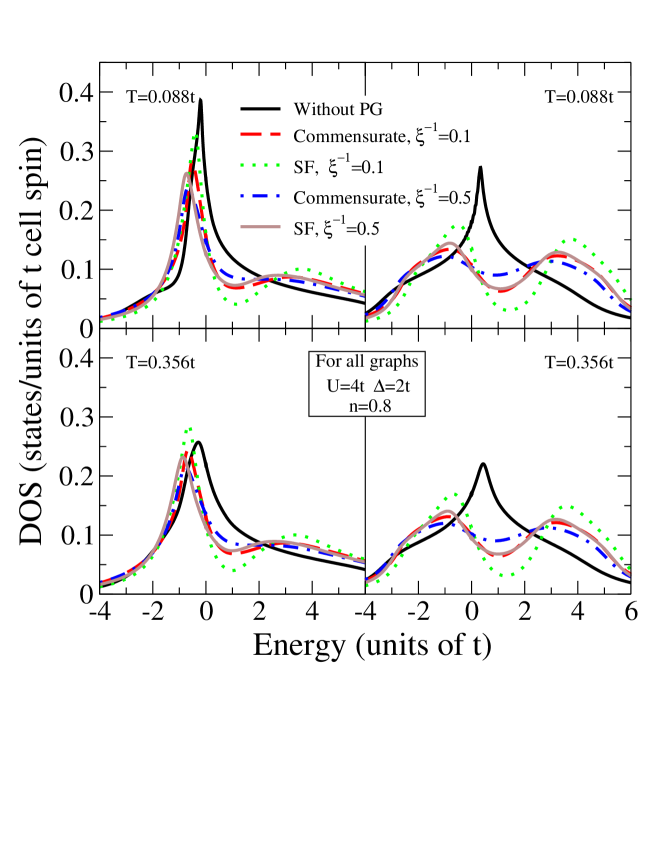
Figure 2: (Color online) Comparison of DOS obtained from DMFT(NRG)+$\Sigma_{\bf k}$ calculations for a filling $n=0.8$, other parameters as in Fig. 1.

The behaviour of the pseudogaps in the DOS has some common features. For example, for $t^{\prime}$=0 at half–filling (Fig. 1, right column) we find that the pseudogap is most pronounced. For $n=0.8$ (Fig. 2, right column) the picture is almost the same but slightly asymmetric. The width of the pseudogap (the distance between peaks closest to Fermi level) appears to be of the order of $\sim 2\Delta$ here. Decreasing the value of $\Delta$ from $2t$ to $t$ leads to a pseugogap that is correspondingly twice smaller and in addition more shallow (see Ref. cm05 ). When one uses the combinatorial factors corresponding to the spin–fermion model (Eq.(12)), we find that the pseudogap becomes more pronounced than in the case of commensurate charge fluctuations (combinatorial factors of Eq. (11)). The influence of the correlation length $\xi$ can be seen is also as expected. Changing from $\xi^{-1}=0.1$ to $\xi^{-1}=0.5$, i.e. decreasing the range of the non-local fluctuations, slightly washes out the pseudogap. Also, increasing the temperature from $T=0.088t$ to $T=0.356t$ leads to a general broadening of the structures in the DOS. These observations remain at least qualitatively valid for $t^{\prime}/t=-0.4$ (Figs. 1 and 2, left columns) with an additional asymmetry due to the next-nearest neighbour hopping. Noteworthy is however the fact that for $t^{\prime}/t=-0.4$ and $\xi^{-1}=0.5$ the pseudogap has almost disappeared for the temperatures studied here. Also very remarkable point is the similarity of the results obtained with the generalized DMFT+$\Sigma_{\bf k}$ approach with $U=4t$ (smaller than the bandwidth $W$) to those obtained earlier without Hubbard–like Coulomb interactions Sch ; KS .

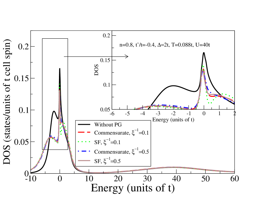
Figure 3: (Color online) Comparison of DOS obtained from DMFT(NRG)+$\Sigma_{\bf k}$ calculations for $t^{\prime}/t=-0.4$, $T=0.088t$, $U=40t$, $\Delta=2t$ and filling $n=0.8$.

Let us now consider the case of a doped Mott insulator. The model parameters are $t^{\prime}/t=-0.4$ with filling $n=0.8$, but the Coulomb interaction strength is now set to $U=40t$. Characteristic features of the DOS for such a strongly correlated metal are a strong separation of lower and upper Hubbard bands and a Fermi level crossing by the lower Hubbard band (for non–half–filled case). Without non-local fluctuations the quasi-particle peak is again formed at the Fermi level; but now the upper Hubbard band is far to the right and does not touch the quasiparticle peak (as it was for the case of small Coulomb interactions). DOS without non-local fluctuations are again presented as black lines in Fig. 3. Results for the case $t^{\prime}=0$ are presented elsewhere cm05 .

With rather strong non-local fluctuations $\Delta=2t$, a pseudogap appears in the middle of quasiparticle peak. In addition we observe that the lower Hubbard band is slightly broadened by fluctuation effects. Qualitative behaviour of the pseudogap anomalies is again similar to those described above for the case of $U=4t$, e.g. a decrease of $\xi$ makes the pseudogap less pronounced, reducing $\Delta$ from $\Delta=2t$ to $\Delta=t$ narrows of the pseudogap and also makes it more shallow etc. (see Ref. cm05 ). Note that for the doped Mott–insulator we find that the pseudogap is remarkably more pronounced for the SDW–like fluctuations than for CDW–like fluctuations.

There are, however, obvious differences to the case with $U=4t$. For example, the width of the pseudogap appears to be much smaller than $2\Delta$, beeing of the order of $\Delta/2$ instead (see Fig. 3). This effect we attribute to the fact that the quasiparticle peak itself is actually strongly narrowed now by local correlations.

IV.3 Generalized DMFT+$\Sigma_{\bf k}$ approach: spectral functions $A(\omega,{\bf k})$

In the previous subsections we discussed the densities of states obtained self–consistently by the DMFT+$\Sigma_{\bf k}$ approach. Once we get a self–consistent solution of the DMFT+$\Sigma_{\bf k}$ equations with non-local fluctuations we can of course also compute the spectral functions $A(\omega,{\bf k})$

$$A(\omega,{\bf k})=-\frac{1}{\pi}{\rm Im}\frac{1}{\omega+\mu-\varepsilon({\bf k})-\Sigma(\omega)-\Sigma_{\bf k}(\omega)},$$ (15)

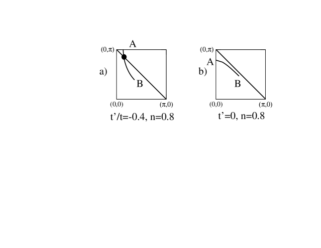
Figure 4: 1/8-th of the bare Fermi surfaces for the occupancy $n=0.8$ and different combinations ($t,t^{\prime}$) used for the calculation of spectral functions $A({\bf k},\omega)$. The diagonal line corresponds to the umklapp surface. The full circle marks the so-called “hot–spot”.

where self–energy $\Sigma(\omega)$ and chemical potential $\mu$ are calculated self–consistently as described in Sec. II. To plot $A(\omega,{\bf k})$ we choose ${\bf k}$–points along the “bare” Fermi surfaces for different types of lattice spectra and filling $n=0.8$. In Fig. 4 one can see corresponding shapes of these “bare” Fermi surfaces (presented are only 1/8-th of the Fermi surfaces within the first quadrant of the first Brillouin zone).

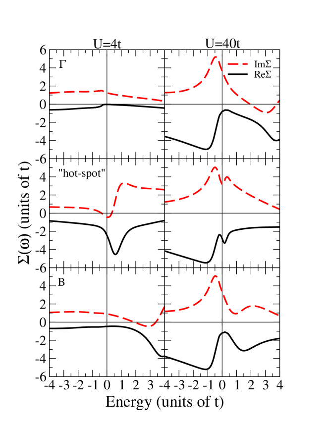
Figure 5: (Color online) Real (dashed line) and imaginary (full line) parts of the self-energy $\Sigma({\bf k},\omega)$ for $t/t^{\prime}=-0.4$, $U=4t$ (left column) and $U=40t$ (right column) for characteristic ${\bf k}$-points: $\Gamma$, “hot-spot” (see Fig. 4) and “cold-spot” (point “B” in Fig. 4). For all graphs the filling is $n=0.8$, temperature $T=0.088t$, inverse correlation length $\xi^{-1}=0.1$, value of pseudogap potential $\Delta=2t$, and SF combinatorics.

A first natural quantity to inspect is the self-energy $\Sigma({\bf k},\omega+i\delta)$, shown in Fig. 5 for $t^{\prime}/t=-0.4$, $n=0.8$ and $U=4t$ (left column) and $U=40t$ (right column). As representative ${\bf k}$-points we chose the centre of the first Brillouin zone ($\Gamma$), the “hot-spot” and “cold-spot” (point “B” in Fig. 4). The results were obtained with NRG at a temperature $T=0.088t$. The structures for $U=4t$ are rather broad, but reveal after a closer inspection features similar to the case $U=40t$. For the latter, the behaviour at $\Gamma$ and “B” is very different from the structures at the “hot-spot”. Namely, while for the former two ${\bf k}$-points ${\rm Im}\Sigma({\bf k},\omega+i\delta)$ shows a nice parabolic maximum at the Fermi energy, the latter develops a minimum instead. Such a structure in the self-energy will result in a rather evident (pseudo) gap in the spectral function at this k-point and weaker pseudogap behaviour in the DOS. Its appearance is obviously due to the presence of the spin-fluctuations at the “hot-spot”. Note that similar features have been observed in numerically expensive cluster mean-field calculations mpj03 , too, with an interpretation as spin-fluctuation induced based on physical expectations. Our calculations, obtained at a minimum numerical expense, indeed show, that including short-ranged fluctuations will precisely produce these non Fermi-liquid structures in the one-particle self-energy. This behaviour is quite typical for the problem and was observed by other groups using different methodsKyung05 ; Stanescu03 ; Katanin04 ; RM . In several works midgap peak in the pseudogap was obtained with explanation of its origin by particular shape of the self-energy close to the Fermi levelKatanin04 ; Stanescu03 ; Barisic05 .

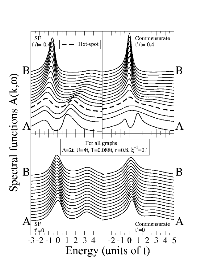
Figure 6: Spectral functions $A({\bf k},\omega)$ obtained from the DMFT(NRG)+$\Sigma_{\bf k}$ calculations along the directions shown in Fig. 4. Model parameters were chosen as $U=4t$, $n=0.8$, $\Delta=2t$, $\xi^{-1}=0.1$ and temperature $T=0.088t$. The “hot–spot” k-point is marked as fat dashed line. The Fermi level corresponds to zero.

In the following we concentrate mainly on the case $U=4t$ and filling $n=0.8$ (Fermi surface of Fig. 4(a)). The corresponding spectral functions $A(\omega,{\bf k})$ are depicted in Fig. 6. When $t^{\prime}/t=-0.4$ (upper row), the spectral function close to the Brillouin zone diagonal (point B) has the typical Fermi–liquid behaviour, consisting of a rather sharp peak close to the Fermi level. In the case of SDW–like fluctuations this peak is shifted down in energy by about $-0.5t$ (left upper corner). In the vicinity of the “hot–spot” the shape of $A(\omega,{\bf k})$ is completely modified. Now $A(\omega,{\bf k})$ becomes double–peaked and non–Fermi–liquid–like. Directly at the “hot–spot”, $A(\omega,{\bf k})$ for SDW–like fluctuations has two equally intensive peaks situated symmetrically around the Fermi level and split from each other by $\sim 1.5\Delta$ Refs. Sch ; KS . For commensurate CDW–like fluctuations the spectral function in the “hot–spot” region has one broad peak centred at the Fermi level with width $\sim\Delta$. Such a merging of the two peaks at the “hot–spot” for commensurate fluctuations was previously observed in Ref. KS . However close to point A this type of fluctuations also produces a double–peak structure in the spectral function.

Spectral functions for the case of $U=4t$ at half–filling ($n=1$) and for $t^{\prime}/t=-0.4$ are similar to those just discussed for $n=0.8$. However, the pseugogap is more pronounced in this case and remains open everywhere close to the umklapp surface for SDW fluctuations cm05 .

In the lower panel of Fig. 6 we show spectral functions for 20% hole doping ($n=0.8$) and the case of $t^{\prime}=0$ (Fermi surface from Fig. 4(b)). Since the Fermi surface now is close to the umklapp surface, the pseudogap anomalies are rather strong and almost non–dispersive along the Fermi surface. At half–filling for $t^{\prime}=0$ the Fermi surface actually coincides with umklapp surface (in case of perfect “nesting” whole Fermi surface is the “hot–region”). The spectral functions are now symmetric around the Fermi level. For SDW–like fluctuations there are two peaks split by $\sim 1.5\Delta$. Again, CDW–like fluctuations give just one peak centred at the Fermi level with width $\sim\Delta$.

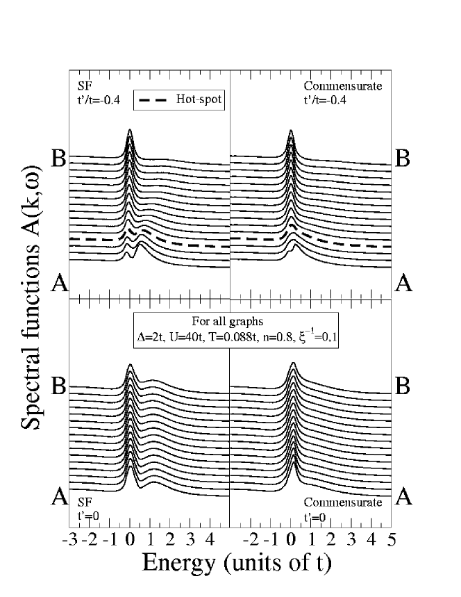
Figure 7: Spectral functions $A({\bf k},\omega)$ obtained from the DMFT(NRG)+$\Sigma_{\bf k}$ calculations for $U=40t$, other parameters as in Fig. 6.

For the case of a doped Mott insulator ($U=40t$, $n=0.8$), the spectral functions obtained by the DMFT+$\Sigma_{\bf k}$ approach are presented in Fig. 7. Qualitatively, the shapes of these spectral functions are similar to those shown in Fig. 6. As was pointed out above, the strong Coulomb correlations lead to a narrowing of the quasiparticle peak and a corresponding decrease of the pseudogap width. As is evident from Fig. 7 the structures connected to the pseudogap are now spread in an energy interval $\sim t$, while for $U=4t$ they are restricted to an interval $\sim 4t$ instead. One should also note that in contrast to $U=4t$ the spectral functions are now about four times less intensive, because part of the spectral weight is transferred to the upper Hubbard band located at about $40t$ and well separated from the quasiparticle peak now.

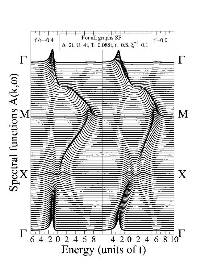
Figure 8: Spectral functions $A({\bf k},\omega)$ obtained from the DMFT(NRG)+$\Sigma_{\bf k}$ calculations along high-symmetry directions of first Brillouin zone $\Gamma(0,0)\!-\!\rm{X}(\pi,0)\!-\!\rm{M}(\pi,\pi)\!-\!\Gamma(0,0)$, SF combinatorics (left row) and commensurate combinatorics (right column). Other parameters are $U=4t$, $n=0.8$, $\Delta=2t$, $\xi^{-1}=0.1$ and temperature $T=0.088t$. The Fermi level corresponds to zero.

Using another quite common choice of ${\bf k}$–points we can compute $A(\omega,{\bf k})$ along high–symmetry directions in the first Brillouin zone: $\Gamma(0,0)\!-\!\rm{X}(\pi,0)\!-\!\rm{M}(\pi,\pi)\!-\!\Gamma(0,0)$. The spectral functions for these ${\bf k}$–points are collected in Fig.  8 for the case of SDW–like fluctuations. Characteristic curves for doped Mott insulator are presented in Ref.cm05 . For all sets of parameters one can see a characteristic double – peak pseudogap structure close to the $X$ point. In the middle of $M\!-\!\Gamma$ direction (so called “nodal” point) one can see the reminiscence of AFM gap which has its biggest value here in case of perfect antiferromagnetic ordering. Also in the nodal point “kink”-like behaviour is observed caused by interactions between correlated electrons with short–range pseudogap fluctuations. A change of the filling leads mainly to a rigid shift of spectral functions with respect to the Fermi level.

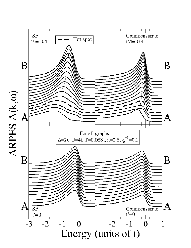
Figure 9: ARPES spectra simulated by multiplication of the spectral functions obtained from DMFT(NRG)+$\Sigma_{\bf k}$ calculations for $U=4t$ and $n=0.8$ Fig. 6 with Fermi function at $T=0.088t$ plotted along the lines in the first BZ as depicted by Fig. 4. All other parameters are the same as in Fig. 6.

With the spectral functions we are now of course in a position to calculate angle resolved photoemission spectra (ARPES), which is the most direct experimental way to observe pseudogap in real compounds. For that purpose, we only need to multiply our results for the spectral functions with the Fermi function at temperature $T=0.088t$. Typical example of the resulting DMFT+$\Sigma_{\bf k}$ ARPES spectra are presented in Fig. 9. More figures of ARPES-like results obtained within the DMFT+$\Sigma_{\bf k}$ approach for a variety of parameters can be found in Ref. cm05 . One should note that for $t^{\prime}/t=-0.4$ (upper panel of Fig. 9) as ${\bf k}$ goes from point “A” to point “B” the peak situated slightly below the Fermi level changes its position and moves down in energy. Simultaneously it becomes more broad and less intensive. The dotted line guides the motion of the peak maximum. Also at the “hot–spot” and further to point “B” one can see some signs of the double–peak structure. Such behaviour of the peak in the ARPES is rather reminiscent of those observed experimentally in underdoped cuprates MS ; Sch ; Kam .

V Conclusion

To summarize, we propose a generalized DMFT+$\Sigma_{\bf k}$ approach, which is meant to take into account the important effects of non–local correlations (in principle of any type) in addition to the (essentially exact) treatment of local dynamical correaltions by the DMFT. In the standard DMFT the “bath” surrounding the effective single Anderson impurity is spatially uniform since the DMFT self-energy is only energy-dependent. The main idea of our extension is to introduce non-local correlations through the “bath”, i.e. to make it spatially non-uniform, while keeping standard DMFT self-consistency equations. Such a generalization of the DMFT allows to supplement it with a ${\bf k}$–dependent self–energy $\Sigma({\bf k},\omega)$. It in turn opens the possibility to access the physics of low–dimensional strongly correlated systems, where different types of spatial fluctuations (e.g. of some order parameter) become important, in a non-perturbative way at least with respect to the important local dynamical correlations. However, we must stress that our procedure in no way introduces any kind of systematic $1/d$–expansion, being only a qualitative method to include a length scale into DMFT. Nevertheless we believe that such a technique can give valuable insight into the physical processes leading to correlation induced $k$-dependent structures in single-particle properties.

In this work we model such effects for the two-dimensional Hubbard model by incorporating into the “bath” scattering of fermions from non-local collective SDW–like antiferromagnetic spin (or CDW–like charge) short-range fluctuations. The corresponding ${\bf k}$–dependent self–energy $\Sigma({\bf k},\omega)$ is obtained from a non-perturbative iterative scheme Sch ; KS . Such choice of the $\Sigma({\bf k},\omega)$ allows to address the problem of pseudogap formation in the strongly correlated metallic state. We showed evidence that the pseudogap appears at the Fermi level within the quasiparticle peak, introducing a new small energy scale of the order of psedogap potential value $\Delta$ in the DOS and more pronounced in spectral functions $A(\omega,{\bf k})$. Let us stress, that our generalization of DMFT leads to non–trivial and in our opinion physically sensible ${\bf k}$–dependence of spectral functions. Is is significant that this particular choice of $\Sigma({\bf k},\omega)$Sch ; KS does not cause difficulties to “double counting” problem within our combined DMFT+$\Sigma_{\bf k}$ approach. Also, the combination of diagrammatically correct techniques like DMFTMetzVoll89 ; vollha93 ; pruschke ; georges96 ; PT and the non-local self-energy ansatz of Refs.Sch ; KS preserves the correct analytical properties of the combined self-energy $\Sigma(i\omega)+\Sigma_{\bf k}(i\omega)$, as well as of the corresponding one-electron propagator (1).

Of course our pseudogap observations are not entirely new. Similar results about pseudogap formation in the 2d Hubbard model were already obtained within cluster DMFT extensions, i.e. the dynamical cluster approximation (DCA)TMrmp ; mpj03 and cellular DMFT (CDMFT) Kyung05 ; CivKot , CPT Gross94 ; Senechal00 ; Senechal05 and two interacting Hubbard sites selfconsistently embedded in a bath Stanescu03 . However, these methods have generic restrictions concerning the size of the cluster, temperatures or filling accessible and, in case of the QMC, values of the local Coulomb energy. Recently, also the EDMFT was applied to demonstrate pseudogap formation in the DOS due to dynamic Coulomb correlationsHW . Note, however, that within the EDMFT there is no way to obtain a ${\bf k}$–dependence in spectral functions beyond that originating from the bare electronic energy dispersion. Important progress was also made with weak coupling approaches for the Hubbard model KyTr and functional renormalization group Katanin04 ; RM . In several papers pseudogap formation was described in the framework of the t-J model Prelovsek . A more general scheme for the inclusion of non–local corrections was also formulated within the so called GW extension to the DMFT BAG ; SKot .

While at a first glance the introduction of additional phenomenological parameters (correlation length $\xi$, and $\Delta$) through the definition of $\Sigma({\bf k},\omega)$ seems to be a step back with respect the methods outlined above, it actually opens the possibility to systematically distinguish between different types of nonlocal fluctuations and their effects and helps to analyze experimental or theoretical data obtained within more advanced schemes in terms of intuitive physical pictures. Note, however, that in principle even the paramters $\xi$ and $\Delta$ can be calculated from the original modelVT , too.

An essential advantage of the proposed combination of two non-perturbative methods (DMFT and $\Sigma({\bf k},\omega)$ from Refs.Sch ; KS ) removes the restrictions on model parameters in e.g. cluster mean-field theories. Our scheme works for any Coulomb interaction strength $U$, pseudogap strength $\Delta$, correlation length $\xi$, filling $n$ and bare electron dispersion $\varepsilon({\bf k})$ on a 2d square lattice for any set of ${\bf k}$-points. Although we presented only high-temperature data in this paper, the possibility to use Wilson’s NRG to solve the effective impurity model also opens the possibiltiy to study properties at $T=0$, which is currently impossible within the DCA or CDMFT for larger clusters. Moreover, the DMFT+$\Sigma_{\bf k}$ approach can be easlily generalized to orbital degrees of freedom, phonons, impurities, etc.

As a further application of our generalized DMFT+$\Sigma_{\bf k}$ we would like to bring readers attention to RefKuchinskii05 , dealing with the problem of Fermi surface destruction in High-T_c compounds because of pseudogap fluctuations.

VI Acknowledgements

We are grateful to A. Kampf for useful discussions. This work was supported in part by RFBR grants 05-02-16301 (MS,EK,IN) 03-02-39024_a (VA,IN), 04-02-16096 (VA,IN), 05-02-17244 (IN), by the joint UrO-SO project $No.$ 22 (VA,IN), and programs of the Presidium of the Russian Academy of Sciences (RAS) “Quantum macrophysics” and of the Division of Physical Sciences of the RAS “Strongly correlated electrons in semiconductors, metals, superconductors and magnetic materials”. I.N. acknowledges support from the Dynasty Foundation and International Centre for Fundamental Physics in Moscow program for young scientists 2005), Russian Science Support Foundation program for young PhD of Russian Academy of Science 2005. One of us (TP) further acknowledges supercomputer support from the Norddeutsche Verbund für Hoch- und Höchstleistungsrechnen.

Appendix A Derivation of generalized DMFT+$\Sigma_{\bf k}$ approach

In this appendix we present a derivation of the generalized DMFT+$\Sigma_{\bf k}$ scheme for the Hubbard model

$$H=-\sum_{ij,\sigma}{t_{ij}c_{i\sigma}^{\dagger}c_{j\sigma}}+U\sum_{i}{n_{i\uparrow}n_{i\downarrow}},$$ (16)

using a diagrammatic approach. The single–particle Green function in Matsubara representation is as usual given by

$$G_{\bf k}(i\omega)=\frac{1}{i\omega+\mu-\varepsilon({\bf k})-\Sigma(i\omega,{\bf k})}$$ (17)

To establish the standard DMFT one invokes the limit of infinite dimensions $d\to\infty$. In this limit only local contributions to electron self–energy survive vollha93 ; georges96 , i.e. $\Sigma_{ij}\to\delta_{ij}\Sigma_{ii}$ or, in reciprocal space, $\Sigma(i\omega,{\bf k})\to\Sigma(i\omega)$.

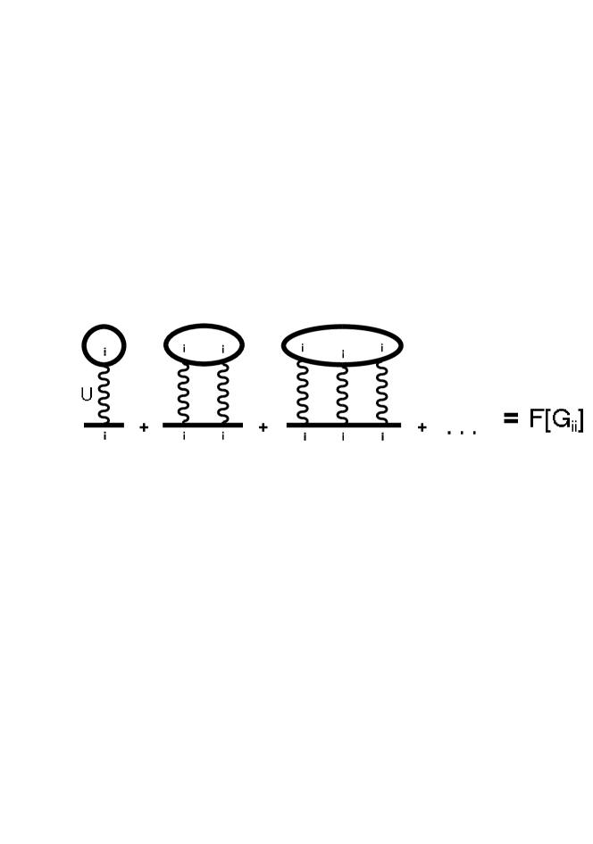
Figure 10: Local “skeleton” diagrams for the DMFT self–energy $\Sigma$. Wavy lines represent the local (Hubbard) Coulomb interaction $U$, full lines denote the local Green function $G_{ii}$.

In Fig. 10 we show examples of “skeleton” diagrams for the local self – energy, contributing in the limit of $d\to\infty$. The complete series of these and similar diagrams defines the local self – energy as a functional of the local Green function

$$\Sigma=F[G_{ii}]\;,$$ (18)

where

$$G_{ii}(i\omega)=\frac{1}{N}\sum_{\bf k}\frac{1}{i\omega+\mu-\varepsilon({\bf k})-\Sigma(i\omega)}.$$ (19)

One then defines the “Weiss field”

$${\cal G}^{-1}_{0}(i\omega)=\Sigma(i\omega)+G^{-1}_{ii}(i\omega)$$ (20)

which is used to set up the effective single impurity problem with an effective action given by (5). Via Dyson’s equation the Green function (4) for this effective single impurity problem can be written as

$$G_{d}(i\omega)=\frac{1}{{\cal G}^{-1}_{0}(i\omega)-\Sigma_{d}(i\omega)}$$ (21)

and the “skeleton” diagrams for self–energy $\Sigma_{d}$ are just the same as shown in Fig. 10, with the replacement $G_{ii}\to G_{d}$. Thus we get

$$\Sigma_{d}=F[G_{d}],$$ (22)

where $F$ is the same functional as in (18). The two equations (21) and (22) define both $G_{d}$ and $\Sigma_{d}$ for a given “Weiss field” ${\cal G}_{0}$. On the other hand, for the local $\Sigma$ and $G_{ii}$ of the initial (Hubbard) problem we have precisely the same pair of equations, viz (18) and (20), and ${\cal G}_{0}$ in both problems is just the same, so that

$$\Sigma=\Sigma_{d};\qquad G_{ii}=G_{d}.$$ (23)

Thus, the task of finding the local self–energy of the $(d\to\infty)$ Hubbard model is eventually reduced to the calculation of the self–energy of an effective quantum single impurity problem defined by effective action of Eq. (5).

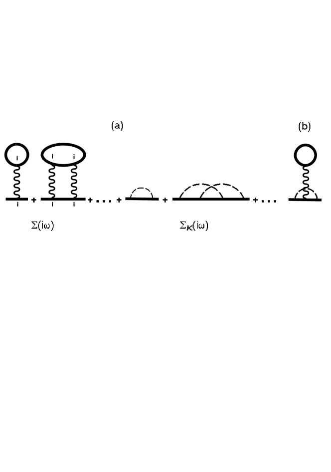
Figure 11: Typical “skeleton” diagrams for the self–energy in the DMFT+$\Sigma_{\bf k}$ approach. The first two terms are DMFT self–energy diagrams; the middle two diagrams show contributions to the non-local part of the self–energy from spin fluctuations (see sectionIII) represented as dashed lines; the last diagram (b) is an example of neglected diagram’s leading to interference between the local and non-local parts.

Consider now non – local contribution to the self – energy. If we neglect interference between local and non–local contributions (as given e.g. by the diagram shown in Fig.11(b)), the full self–energy is approximately determined by the sum of these two contributions. “Skeleton” diagrams for the non-local part of the self–energy, $\Sigma_{\bf k}(i\omega)$, are then those shown in Fig. 11(a), where the full line denotes the Green function $G_{\bf k}$ of Eq. (1), while broken lines denote the interaction with static Gaussian spin (charge) fluctuations. These diagrams are just absent within the standard DMFT (as any contribution from Ornstein – Zernike type fluctuations vanish for $d\to\infty$), and no double counting problems arise at all.

The local contribution to the self–energy is again defined by the functional (18) via the local Green function $G_{ii}$, which is now given by (2). Introducing again a “Weiss field” via (20) and repeating all previous arguments, we again reduce the task of finding the local part of the self–energy to the solution of an “single impurity” problem with an effective action (5).

To determine the non–local contribution $\Sigma_{\bf k}(i\omega)$ we first introduce

$${\cal G}_{0\bf k}(i\omega)=\frac{1}{G_{\bf k}^{-1}(i\omega)+\Sigma_{\bf k}(i\omega)}=\frac{1}{i\omega+\mu-\varepsilon({\bf k})-\Sigma(i\omega)}$$ (24)

as the “bare” Green function for electron scattering by static Gaussian spin (charge) fluctuations. The assumed static nature of these fluctuations allows to use the method of Refs.Sch ; KS ; MS79 and the calculation of the non–local part of the self–energy $\Sigma_{\bf k}(i\omega)$ reduces to the recursion procedure defined by Eqs. (9) and (8). The choice of the “bare” Green function Eq. (24) guarantees that the Green function “dressed” by fluctuations $G_{\bf k}^{-1}(i\omega)={\cal G}_{0\bf k}^{-1}(i\omega)-\Sigma_{\bf k}(i\omega)$, which enters into the “skeleton” diagrams for $\Sigma_{\bf k}(i\omega)$, just coincides with the full Green functions $G_{\bf k}(i\omega)$.

Thus we obtain a fully self–consistent scheme to calculate both local (due to strong single–site correlations) and non–local (due to short–range fluctuations) contributions to electron self–energy.

Appendix B $\Delta$ in the Hubbard model.

In this Appendix we derive the explicit microscopic expression for pseudogap amplitude $\Delta$ given in (13). Within the two–particle self–consistent approach of Ref. VT , valid for medium values of $U$, and neglecting charge fluctuations, we can write down an expression for the electron self–energy of the form used in (1), with

$$\Sigma_{\sigma}(i\omega)=Un_{-\sigma}$$ (25)

as the lowest order local contribution due to the on–site Hubbard interaction, surviving in the limit of $d\to\infty$, and exactly accounted for in DMFT (with all higher–order contributions). Non–local contribution to the self–energy (vanishing for $d\to\infty$ and not accounted within DMFT) due to interaction with spin–fluctuations then leads to the expression

$$\Sigma_{\vec{k}}(i\omega)=\frac{U}{4}\frac{T}{N}\sum_{m}\sum_{\bf q}U_{sp}\chi_{sp}({\bf q},\nu_{m})G_{0}({{\bf{k+q}},i\omega+i\nu_{m}})\;,$$ (26)

where

$$U_{sp}=g_{\uparrow\downarrow}(0)U,\qquad g_{\uparrow\downarrow}(0)=\frac{<n_{i\uparrow}n_{i\downarrow}>}{<n_{i\uparrow}><n_{i\downarrow}>}$$ (27)

with $<n^{2}_{\sigma}>=<n_{\sigma}>$ and $<n_{i\uparrow}>=<n_{i\downarrow}>=\frac{1}{2}n$ in the paramagnetic phase. For the dynamic spin susceptibility $\chi_{sp}({\bf q},\nu_{m})$ we use the standard Ornstein–Zernike form VT , similar to that used in spin–fermion model Sch , which describes enhanced scattering with momenta transfer close to antiferromagnetic vector ${\bf Q}=(\pi/a,\pi/a)$. With these approximations, we can write down the following expression for the non–local contribution to the self–energy Sch ; KS :

$$\Sigma_{\vec{k}}(i\omega)=\frac{1}{4}UU_{sp}\frac{T}{N}\sum_{m}\sum_{\vec{q}}\chi_{sp}({\bf q},\nu_{m})\frac{1}{i\omega+i\nu_{m}+\mu-\varepsilon({\bf k+q})}\approx$$

$$\approx\frac{1}{4}UU_{sp}\frac{T}{N}\sum_{m}\sum_{\vec{q}}\chi_{sp}({\bf q},\nu_{m})\sum_{\vec{q}}S({\vec{q}})\frac{1}{i\omega+\mu-\varepsilon({\bf k+q})}\equiv$$

$$\equiv\Delta^{2}\sum_{\vec{q}}S({\bf q})\frac{1}{i\omega+\mu-\varepsilon({\bf k+q})}=$$

$$=\frac{\Delta^{2}}{i\omega+\mu-\varepsilon({\bf p+Q})+i(|v^{x}_{\bf p+Q}|+|v^{y}_{\bf p+Q}|)\kappa{\rm sign}\omega}.$$ (28)

Here we have introduced the static form factor KS

$$S({\vec{q}})=\frac{2\xi^{-1}}{(q_{x}-Q_{x})^{2}+\xi^{-2}}\frac{2\xi^{-1}}{(q_{y}-Q_{y})^{2}+\xi^{-2}}$$ (29)

and the squared pseudogap amplitude

$$\Delta^{2}=\frac{1}{4}UU_{sp}\frac{T}{N}\sum_{m}\sum_{\vec{q}}\chi_{sp}({\bf q},\nu_{m})=$$

$$=\frac{1}{4}UU_{sp}[<n_{i\uparrow}>+<n_{i\downarrow}>-2<n_{i\uparrow}n_{i\downarrow}>]=$$

$$=\frac{1}{4}UU_{sp}\frac{1}{3}<{\vec{S}}_{i}^{2}>,$$ (30)

where we have used the exact sum–rule for the susceptibility Sch ; VT . Taking into account (27) we immediately obtain (13).

Actually, the approximations made in (28) and (29) allow for an exact summation of the whole Feynman series for electron interaction with spin–fluctuations, replaced by the static Gaussian random field. Thus generalizing the one–loop approximation (28) eventually leads to the basic recursion procedure given in (9), (8) Refs. Sch ; KS .

Using the DMFT(QMC) approach we computed occupancies $<n_{i\uparrow}>$, $<n_{i\downarrow}>$ and double occupancies $<n_{i\uparrow}n_{i\downarrow}>$ required to calculate the pseudogap amplitude $\Delta$ of Eq. (30) In Fig. 12 the corresponding values of $\Delta$ are presented. One can see that $\Delta$ grows when the filling goes to $n=1$. While $U$ approaches $8t$ (the value of the bandwidth for a square lattice) $\Delta$ as a function of $n$ grows monotonically. When $U$ becomes larger than $W=8t$ (when a metal–insulator transition occurs) one can see a local minimum for $n=0.9$, which becomes more pronounced with further increase of $U$. For $t^{\prime}/t=-0.4$ and both temperatures the scatter of $\Delta$ values is smaller than for the case of $t^{\prime}=0$. Also $\Delta$ has a rather weak temperature dependence. All values of $\Delta$ lie in the interval $\sim 0.75t\div 2t$. Therefore, for our computations we took only two characteristic values of $\Delta=t$ and $\Delta=2t$.

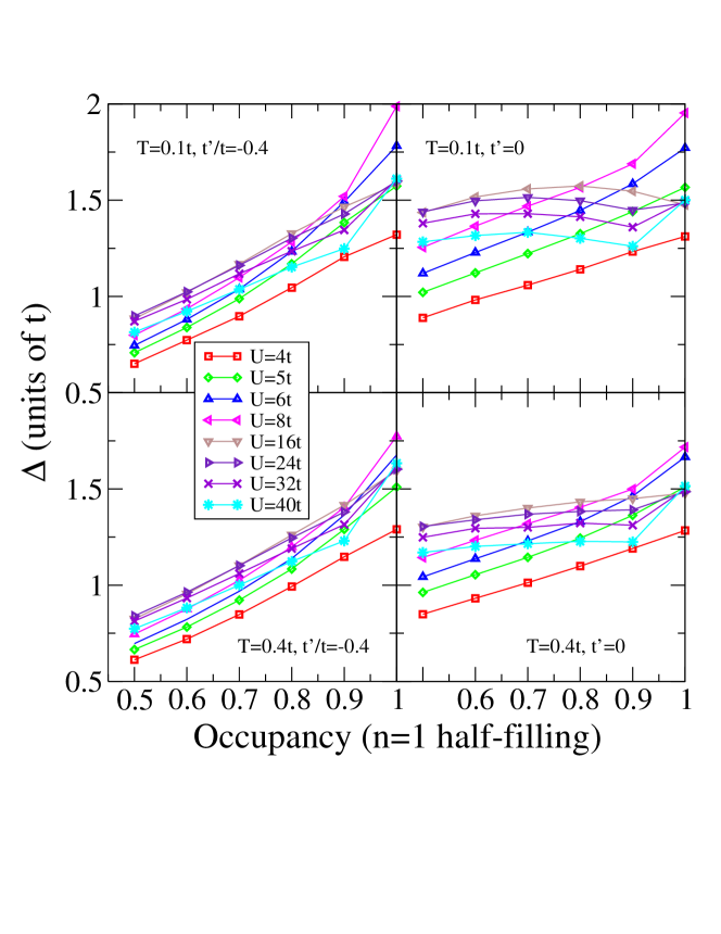
Figure 12: (Color online) Filling dependence of the pseudo gap potential $\Delta$ calculated with DMFT(QMC) for varying Coulomb interaction ($U$) and temperature ($T$) on a two–dimensional square lattice with two sets of ($t,t^{\prime}$).

References

- (1) T. Timusk, B. Statt, Rep. Progr. Phys, 62, 61 (1999).
- (2) M. V. Sadovskii, Usp. Fiz. Nauk 171, 539 (2001) [Physics – Uspekhi 44, 515 (2001)].
- (3) D. Pines, ArXiv: cond-mat/0404151.
- (4) J. Schmalian, D. Pines, B.Stojkovic, Phys. Rev. Lett. 80, 3839 (1998); Phys. Rev. B 60, 667 (1999).
- (5) E. Z. Kuchinskii, M. V. Sadovskii, Zh. Eksp. Teor. Fiz. 115, 1765 (1999) [(JETP 88, 347 (1999)]. (available as ArXiv: cond-mat/9808321)
- (6) W. Metzner and D. Vollhardt, Phys. Rev. Lett. 62, 324 (1989).
- (7) D. Vollhardt, in Correlated Electron Systems, edited by V. J. Emery, World Scientific, Singapore, 1993, p. 57.
- (8) Th. Pruschke, M. Jarrell, and J. K. Freericks, Adv. in Phys. 44, 187 (1995).
- (9) A. Georges, G. Kotliar, W. Krauth, and M. J. Rozenberg, Rev. Mod. Phys. 68, 13 (1996).
- (10) G. Kotliar and D. Vollhardt, Physics Today 57, No. 3 (March), 53 (2004).
- (11) Q. Si and J.L. Smith, Phys. Rev. Lett. 77, 3391 (1996).
- (12) Th. Maier, M. Jarrell, Th. Pruschke and M. Hettler, Rev. Mod. Phys. (in print, ArXiv: cond-mat/0404055).
- (13) G. Kotliar, S.Y. Savrasov, G. Palsson, G. Biroli, Phys. Rev. Lett. 87, 186401 (2001); For periodized version (PCDMFT) see M. Capone, M. Civelli, S.S. Kancharla, C. Castellani, and G. Kotliar, Phys. Rev. B 69, 195105 (2004).
- (14) C. Gros, and R. Valenti, Annalen der Phys. 3, 460 (1994).
- (15) D. Senechal, D. Perez, and M. Pioro-Ladri re, Phys. Rev. Lett. 84, 522 (2000); D. Senechal, D. Perez, and D. Plouffe, Phys. Rev. B 66, 075129 (2002).
- (16) B. Kyung, S.S. Kancharla, D. Senechal, A.-M.S. Tremblay, M. Civelli, G. Kotliar, ArXiv: cond-mat/0502565.
- (17) M. Civelli, M. Capone, S.S. Kancharla, O. Parcollet, G. Kotliar, ArXiv: cond-mat/0411696.
- (18) J. E. Hirsch and R. M. Fye, Phys. Rev. Lett. 56, 2521 (1986); M. Jarrell, Phys. Rev. Lett. 69, 168 (1992); M. Rozenberg, X. Y. Zhang, and G. Kotliar, Phys. Rev. Lett. 69, 1236 (1992); A. Georges and W. Krauth, Phys. Rev. Lett. 69, 1240 (1992); M. Jarrell in Numerical Methods for lattice Quantum Many-Body Problems, edited by D. Scalapino, Addison Wesley, 1997. For review of QMC for DMFT see Ref.Held01 .
- (19) K. Held, I.A. Nekrasov, N. Blümer, V.I. Anisimov, and D. Vollhardt, Int. J. Mod. Phys. B 15, 2611 (2001); K. Held, I.A. Nekrasov, G. Keller, V. Eyert, N. Blümer, A.K. McMahan, R.T. Scalettar, T. Pruschke, V.I. Anisimov, and D. Vollhardt, ArXiv: cond-mat/0112079 (Published in Quantum Simulations of Complex Many-Body Systems: From Theory to Algorithms, eds. J. Grotendorst, D. Marks, and A. Muramatsu, NIC Series Volume 10 (NIC Directors, Forschunszentrum Jülich, 2002) p. 175-209.
- (20) K.G. Wilson, Rev. Mod. Phys. 47, 773 (1975); H.R. Krishna-murthy, J.W. Wilkins, and K.G. Wilson, Phys. Rev. B 21, 1003 (1980); ibid. 21, 1044 (1980); for a comprehensive introduction to teh NRG see e.g. A.C. Hewson, The Kondo Problem to Heavy Fermions (Cambridge University Press, 1993).
- (21) R. Bulla, A.C. Hewson and Th. Pruschke, J. Phys. – Condens. Matter 10, 8365(1998); R. Bulla, Phys. Rev. Lett. 83, 136 (1999).
- (22) M. V. Sadovskii, Zh. Eksp. Teor. Fiz. 77, 2070(1979) [Sov.Phys.–JETP 50, 989 (1979)].
- (23) Y. M. Vilk, A.-M. S. Tremblay, J. Phys. I France 7, 1309 (1997).
- (24) O. Gunnarsson, O. K. Andersen, O. Jepsen, and J. Zaanen, Phys. Rev. B 39, 1708 (1989).
- (25) M. T. Czyzyk and G. A. Sawatzky, Phys. Rev. B49, 14211 (1994).
- (26) M.V. Sadovskii, I.A. Nekrasov, E.Z. Kuchinskii, Th. Prushke, V.I. Anisimov. ArXiv: cond-mat/0502612.
- (27) Th.A. Maier, Th. Pruschke, and M. Jarrell, Phys. Rev. B 66, 075102 (2002).
- (28) T.D. Stanescu and P. Phillips, Phys. Rev. Lett. 91, 017002 (2003).
- (29) A.A. Katanin and A.P. Kampf, Phys. Rev. Lett. 93, 106406 (2004)
- (30) D. Rohe, W. Metzner, Phys. Rev. B71, 115116 (2005).
- (31) D.K. Sunko, S. Barisic, Eur. Phys. J. B 46, 269 (2005).
- (32) A. Kaminski, H. M. Fretwell, M. R. Norman, M. Randeria, S. Rosenkranz, U. Chatterjee, J. C. Campuzano, J. Mesot, T. Sato, T. Takahashi, T. Terashima, M. Takano, K. Kadowaki, Z. Z. Li, H. Raffy, Phys. Rev. B 71, 014517 (2005).
- (33) D. Senechal and A.-M.S. Tremblay, Phys. Rev. Lett. 92, 126401 (2004).
- (34) K. Haule, A. Rosch, J. Kroha, P. Wölfle, Phys. Rev. Lett. 89, 236402 (2002); Phys. Rev. B 68, 155119 (2003).
- (35) B. Kyung, V. Hankevich, A.-M. Dare, A.-M.S. Tremblay. Phys. Rev. Lett. 93, 147004 (2004).
- (36) P. Prelovsek and A. Ramsak, Phys. Rev. B 63, 180506 (2001); P. Prelovsek, A. Ramsak, ArXiv: cond-mat/0502044.
- (37) S. Biermann, F. Aryasetiawan, A. Georges, Phys. Rev. Lett. 90, 086402 (2003).
- (38) P. Sun, G. Kotliar, Phys. Rev. Lett. 92, 196402 (2004).
- (39) E.Z. Kuchinskii, I.A. Nekrasov, M.V. Sadovskii, JETP Letters 82(4), 217 (2005).