Skeleton and fractal scaling in complex networks

Abstract

We find that the fractal scaling in a class of scale-free networks originates from the underlying tree structure called skeleton, a special type of spanning tree based on the edge betweenness centrality. The fractal skeleton has the property of the critical branching tree. The original fractal networks are viewed as a fractal skeleton dressed with local shortcuts. An in-silico model with both the fractal scaling and the scale-invariance properties is also constructed. The framework of fractal networks is useful in understanding the utility and the redundancy in networked systems.

The emerging unifying concepts such as the small-world property ws , the scale-free behavior ba , and the hierarchical modularity ravasz now constitute our basic understanding of the organization of complex networked systems, which appear in as diverse examples as the world-wide web, the social networks, and the biochemical reaction networks inside cells. The small-world property refers to the one that the average separation $\langle D\rangle$ between pairs of vertices in the network scales at most logarithmically in the total number of vertices $N$ in the system, $\langle D\rangle\sim\ln N$. The scale-free behavior means the lack of characteristic scales in the number of links $k$ a vertex has, called the degree, manifesting itself in the form of a power-law degree distribution $p_{d}(k)\sim k^{-\gamma}$ for large $k$. Recent discovery of fractal scaling and topological self-similarity in the world-wide web and the metabolic networks ss , however, raised a new perspective on our view of such networked systems. The fractal scaling stands for the power-law relation between the minimum number of boxes $N_{B}$ needed to cover the entire network and the size of the boxes $\ell_{B}$,

$$N_{B}(\ell_{B})\sim\ell_{B}^{-d_{B}},$$ (1)

with a finite fractal dimension $d_{B}$ feder . The self-similarity here refers to the scale-invariance of the degree distribution under the coarse-graining with different box sizes (length scales) as well as under the iterative application of the coarse-graining (the network renormalization) ss ; bjkim . It has been observed, however, that not all networks are fractal and the most random network models proposed yet are not fractal, either. This poses a fundamental question on the origin of the fractal scaling observed in the real-world networks ss ; strogatz ; yook ; havlin . In this Letter, we show that the fractal property of the network can be understood from its underlying tree structure.

While highly entangled as a network looks, a more simple structure is embedded underneath it, that is the spanning tree. A spanning tree is a tree composed of $N-1$ edges in a way that they connect all the $N$ vertices in the network. Of particular significance is the so-called skeleton skeleton of a network. The skeleton is a particular spanning tree, which is formed by the edges with highest betweenness centralities freeman ; gn or loads static . The remaining edges in the system are called shortcuts, which contribute to forming loops. The skeleton of a scale-free network is also scale-free but with different $\gamma$. Since the betweenness centrality is related to the amount of information flow along a given edge, the skeleton can be considered as the “communication kernel” of the network skeleton . If a network is organized in a modular way, as it is believed to be so for the world-wide web and the biological systems, the inter-modular connections offer communication channels across the modules, thus gaining high betweenness centralities. By construction, the skeleton is composed preferentially of such high-betweenness inter-modular connections, which will preserve the modular structure while greatly simplifying the complexity. Furthermore, if the modular structure is distinct enough, i.e., there is a rather clear-cut separation between modules, we can expect that even a random spanning tree can capture the modular structure. Thus by looking at the properties of its spanning trees, we can visualize more easily the topological organization of the network.

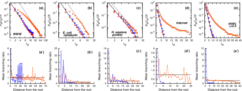
Figure 1: (Color) (a–e) Box counting analysis of original networks ($\circ$, red)) and their skeleton ($\triangledown$, blue) and random spanning tree ($\triangle$, orange). Shown are cases for the world-wide web (a), the metabolic network of Escherichia coli (b), and the protein interaction network of Homo sapiens (c), the Internet at the autonomous systems level as of the year 2004 (d), and the static model network with $\gamma=2.3$ and $\langle k\rangle=4$ (e). In (a–c), we also show two guidelines for the fractal scaling of the original network (black) and its random spanning tree (gray). Slope of each guideline is (a) $-4.1$, (b) $-3.5$, and (c) $-2.3$. In (d–e), the black line is a fit to the exponential function and the gray one is to a power law. (a^′–e^′) Branching analysis. The mean branching number as a function of distance from the root for the skeleton ($\triangledown$, blue) and the random spanning tree ($\triangle$, orange) of the networks in (a–e). For (a^′–c^′), both the skeleton and the random spanning tree fulfill the criticality condition, $\langle m\rangle=1$ (horizontal line), as the distance from the root increases, while for (d^′–e^′), the mean branching number of the skeleton decays to zero with no plateau at $\langle m\rangle=1$.

With the underlying skeleton and random spanning tree, here we perform the fractal scaling analysis by measuring $N_{B}(\ell_{B})$ for several real-world networks and network models method . Comparison of the fractal scalings in each original network with the corresponding spanning trees reveals distinct patterns according to the presence or the absence of fractality in the network. For the fractal networks, such as the world-wide web [Fig. 1(a)] www , the metabolic network of Escherichia coli [Fig. 1(b)] metabolic , and the protein interaction network of Homo sapiens [Fig. 1(c)] dip , the numbers of boxes needed to cover the original network and its skeleton are almost the same. Moreover, the random spanning tree, while possessing a different statistics of $N_{B}$, shows nevertheless the same fractal dimension $d_{B}$. This is surprising, because in the world-wide web, for example, more than $2N$ edges (shortcuts) are added onto the skeleton (the average degree of the world-wide web is $6.7$), which is a tremendous number in the graph-theoretical sense, and by no means a minute perturbation. Such a robustness of fractal scaling in the world-wide web shows that even though the network is far from being a tree, the shortcuts are distributed in a way that they preserve the fractality and modularity. In other words, shortcuts are mainly present inside modules and the connections between different modules are largely made through the skeleton. This topological structure can be measured by the fraction of intra-branch shortcuts among the total number of shortcuts, a branch being the subtree connected to the most connected vertex. We find that the ratio is 0.78, 0.33, and 0.45 for Figs. 1(a), 1(b), and 1(c), respectively. On the other hand, other networks exhibit different features in the fractal scaling analysis. For example, the Internet autonomous systems [Fig. 1(d)] or the static model with $\gamma=2.3$ and $\langle k\rangle=4$ [Fig. 1(e)], the box counting number of the original network and the skeleton decays with $\ell_{B}$ much faster than that of the random spanning tree, and the fraction of intra-branch shortcuts is small: 0.087 for Fig. 1(d) and 0.015 for Fig. 1(e). Also for the social networks, such as the actor network and the collaboration network, the $N_{B}(\ell_{B})$ curves are appreciably different from those of the skeletons, implying that the global topology of the social network is highly interwoven on a large scale to form a more compact structure som .

The scaling behavior of the box counting relation Eq. (1) in Figs. 1(a)–1(c) for the original network and its skeleton suggests that the fractal property of the network originates from that of the skeleton. In addition, we argue here that the criticality in the topology of the skeleton is required for a network to be a fractal: The tree structures such as the skeleton and the random spanning tree may be seen as generated through a multiplicative branching process starting from a root vertex harris . At each branching step, each vertex born in the previous step generates $m$ offsprings with probability $b_{m}$. The criticality condition means the average branching number,

$$\langle m\rangle\equiv\sum_{m=0}^{\infty}mb_{m}=1.$$ (2)

Thus the branching tree grows perpetually with offsprings neither flourishing nor dying out. In this case, when $b_{m}\sim m^{-\gamma}$, the number of vertices $s$ in the tree scales with its linear size $t$ in a power-law form as $s\sim t^{z}$ with $z=(\gamma-1)/(\gamma-2)$ for $2<\gamma<3$ and $z=2$ for $\gamma>3$ harris ; dslee , and the tree structure is fractal with fractal dimension $d_{B}=z$. Such a critical branching tree is similar in the topological characteristics to the homogeneous scale-free tree network proposed in Ref. burda . To check the validity of our suggestion, we examine if the criticality condition is fulfilled for the skeleton and the random spanning trees of the four real-world networks and the static model in Figs. 1(a^′)–1(e^′). Indeed, for the fractal networks [Figs. 1(a^′)–1(c^′)], both the skeleton and the random spanning tree fulfill the criticality condition, even though in reality, the dynamic origins of their formations may well be more complicated than the pure branching dynamics. In our analysis, the root is taken as the most connected vertex in the tree. On the other hand, for non-fractal networks, the mean number of branches of the skeleton decays to zero rapidly as the distance from the root increases [see Figs. 1(d^′) and 1(e^′)]. A similar behavior is observed for the actor network as well som . Thus the actor network is not a fractal. However, the random spanning tree satisfies the criticality condition in all cases, suggesting the generic fractal structure of this kind of trees as shown in Ref. optimal . In short, a fractal network contains a fractal skeleton underneath it, which is perturbed by local shortcuts, thus preserving its fractal property.

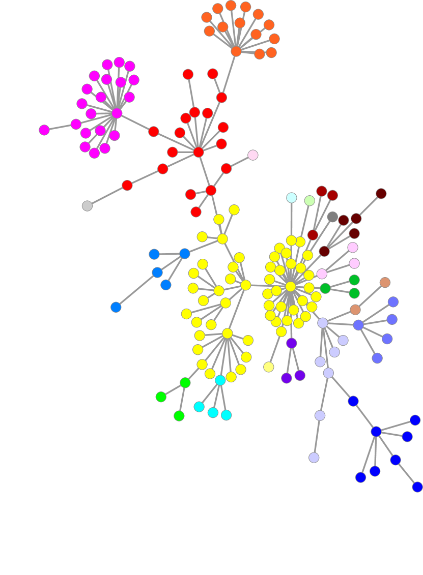
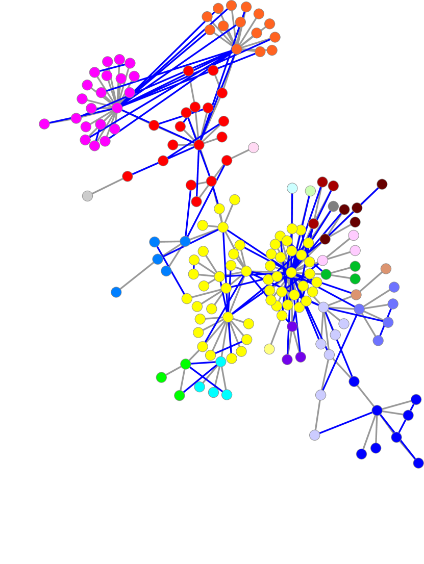
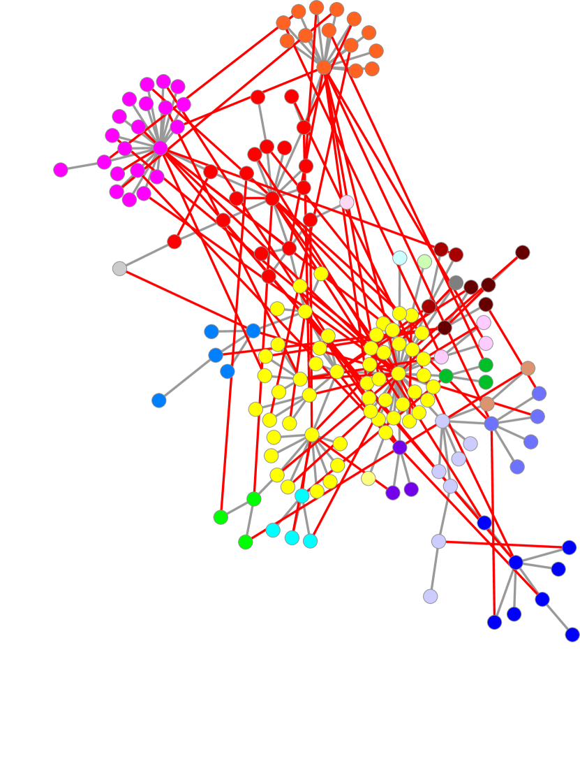
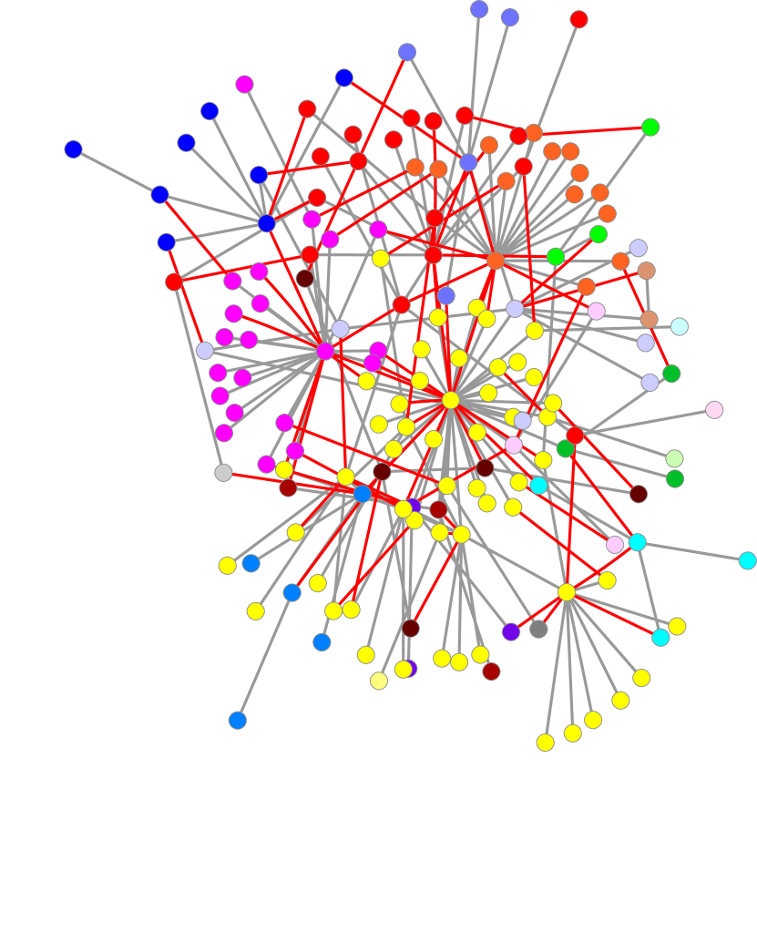
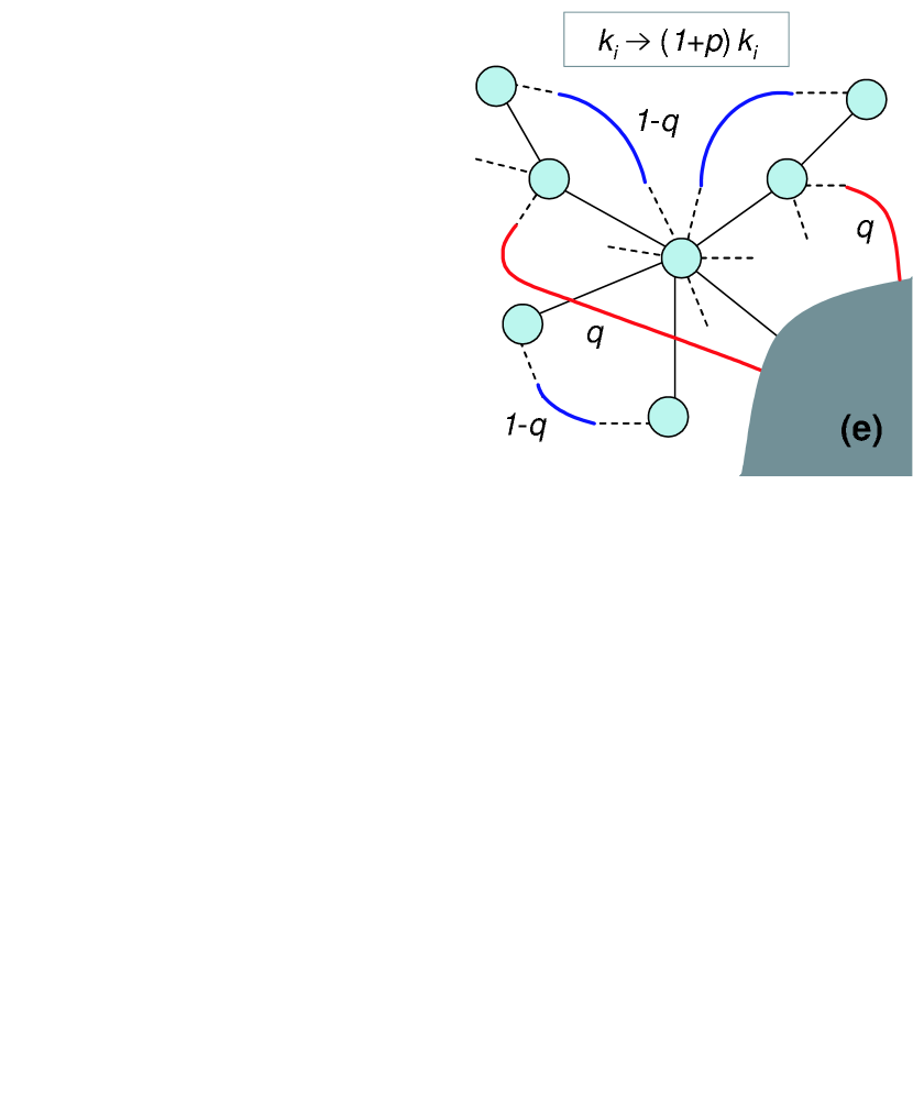
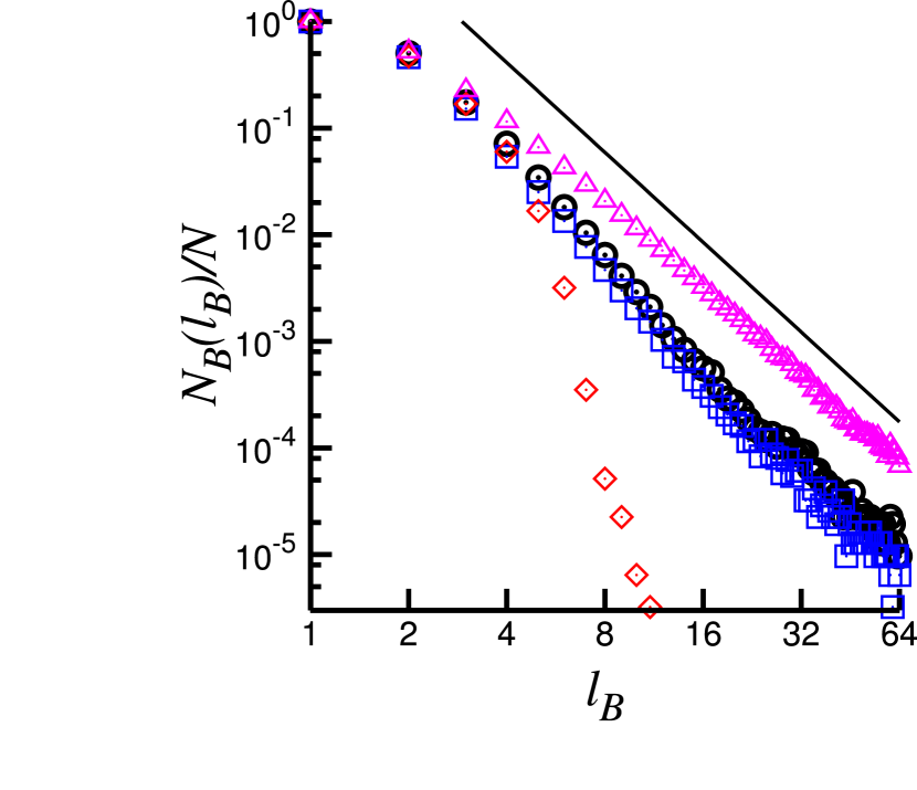
Figure 2: (a) Uncorrelated scale-free tree with the degree exponent $\gamma=2.3$ and the number of vertices $N=164$. It is grown by the multiplicative branching rule harris , with the branching probability $b_{m}\sim m^{-\gamma}$. (b) Fractal model network created by adding local shortcuts (green) to the tree in (a). (c) A non-fractal model network created by adding random shortcuts (blue) allowing global connection. (d) The generic configuration of the network in (c) generated by Pajek, and the absence of inherent modular structure. In (b–d), the color of each vertex is that of the corresponding vertex in (a). (e) Schematic illustration of the growth rule of the fractal network model. The shaded region indicates the rest of the network generated so far. (f) The fractal scaling analysis of networks with larger size $N=311,043$, constructed in the same manner as those in (a)-(c). Squares (blue) correspond to the fractal network model in (b) with $p=0.5$, circles (black) to its skeleton, and the diamonds (red) to the non-fractal network model in (c) with $q=1$. Solid line is the guideline with slope $\approx-2.8$.

Incorporating all the findings so far, we set up a fractal network model. The model is based on the multiplicative branching tree harris . We first introduce an exponent $\gamma$ for the branching probability $b_{m}\sim m^{-\gamma}$ ($m\geq 1$), designed to produce the desired power-law degree distribution $p_{d}(k)\sim k^{-\gamma}$ with $\gamma>2$. The branching probability is properly normalized to be critical, i.e., it satisfies Eq. (2). Next, a parameter $p$ is introduced to control the number of shortcuts added, and hence the mean degree of the network. One final parameter $q$ accounts for the relative frequency of the local and the global shortcuts. The construction of the model network proceeds as follows: i) A tree is grown by the multiplicative branching rule with branching probability $b_{m}$. ii) After the branching process, every vertex increases its degree by a factor $p$ and attempts to make shortcuts to its local neighbors. iii) For each successful shortcut in ii), with probability $q$, we replace it by reconnecting it to a randomly chosen vertex, not restricted to its local neighbors. In the latter case, we choose the vertex with a weight in proportion to its degree in the branching tree, so as to maintain the same power-law scaling of the degree distribution. This rule is schematized in Fig. 2(e) som . Fig. 2(a) is an illustrative example of a branching tree of size $N=164$ and $\gamma={2.3}$. The vertices of the tree are colored according to which box they belong to in a particular box-covering with $\ell_{B}=2$. For such a tree, even a simple graph drawing algorithm, such as Pajek pajek , can capture its inherent hierarchical structure. Fig. 2(b) shows the fractal network structure with the addition of local shortcuts, where we use $p=0.5$ and $q=0$. The hierarchical modular structure presented in the tree network [Fig. 2(a)] persists. On the other hand, the network with $q=1$ shown in Fig. 2(c), in which the same number of shortcuts as in Fig. 2(b) are attached, does not retain the modularity. Such an absence of modularity can be readily seen in Fig. 2(d), a different layout of the same network as Fig. 2(c) generated by Pajek in an unsupervised manner. Consequently, the fractal property is preserved in the case of $q=0$, whereas it is not for $q=1$, as is clearly revealed by the box counting analysis in Fig. 2(f).

It is noteworthy that there exists an important distinction between the present model and other scale-free trees such as the Barabási-Albert tree ba and the geometrically growing scale-free tree jung . Such models are not fractal, because they do not fulfill the criticality condition. Indeed, their mean branching rate decreases to zero monotonically as the branching proceeds, without a plateau at $\langle m\rangle\approx 1$ som . Such a type of tree network was classified as “causal” trees in Ref. causal . Note also that the fractal trees are not small-worlds. However, with a small number of global shortcuts, e.g., $q=0.01$ in our model with $N\sim 3$$\times$$10^{5}$, the network turns into a small world. This is seen in the mean box mass versus $\ell_{B}$ plot in the cluster growing method analysis som .

The fractal network model is self-similar. To check it, we perform the coarse-graining through the box counting method by replacing each box with a single super-node, and connecting them if any of their member vertices is connected ss . We find that the degree distribution of the fractal network model is invariant under the coarse-graining by the boxes with different sizes. In addition, the degree distribution is invariant under successive applications of the coarse-graining transformation som . It is interesting to note that some networks are self-similar, that is, exhibit the scale-invariant degree distribution, yet are not fractal. Typical example of such networks is the Internet som . So the fractality and the self-similarity do not always imply each other in complex networks.

The framework of fractal network is helpful to understand, for example, the utility and the redundancy in the metabolic networks from a purely topological aspect. The high flux backbone in the metabolic network of E. coli obtained through the flux balance analysis was shown to be composed of many branches with few inter-branch connections and to merge into the biomass reaction meta . Obviously, its topological shape resembles the branching tree skeleton rooted from a vertex with the largest number of connections if the direction in edge is ignored. On the other hand, recent in silico flux analysis ghim has shown that the metabolic network of E. coli contains high density of backup reactions (redundancies) for a given condition. Such a reaction is barely used in the normal condition, but takes up a high flux when a certain reaction on the backbone is blocked. When the simultaneous blockade of such a reaction pair blocks the biomass production, they are called synthetic lethal epistasis . Most synthetic lethal reactions are located very close to each other, being apart in three reaction steps or less along the metabolic network. Also they are mostly in the same functional category. Thus the reactions with high (low) flux in wild type can be regarded as the edges on the skeleton (shortcuts) in the framework of the fractal network.

The critical branching tree that can be found in various phenomena such as earthquake processes, population and biological dynamics, epidemics, social cascades, etc., also appears in the skeleton of fractal networks, as we found here. While the evolving process of the fractal networks would be complex and diverse depending on the specific systems, the underlying structure, the skeleton, has the topology of the critical branching tree. Identifying such a simple structure underneath is a step forward towards further studies on the renormalization and the universality in complex networks.

This work is supported by the KRF Grant No. R14-2002-059-01000-0 in the ABRL program funded by the Korean government MOEHRD. G.S. gratefully acknowledges financial support from the Swiss National Science Foundation under the fellowship PBEL2-106182.

References

- (1) D. J. Watts, S. H. Strogatz, Nature (London) 393, 440 (1998).
- (2) A.-L. Barabási, R. Albert, Science 286, 509 (1999).
- (3) E. Ravasz, A. L. Somera, D. A. Mongru, Z. N. Oltvai, A.-L. Barabási, Science 297, 1551 (2002).
- (4) C. Song, S. Havlin, H. A. Makse, Nature (London) 433, 392 (2005).
- (5) J. Feder, Fractals (Plenum, New York, 1988).
- (6) B. J. Kim, Phys. Rev. Lett. 93, 168701 (2004).
- (7) S. H. Strogatz, Nature (London), 433, 365 (2005).
- (8) S.-H. Yook, F. Radicchi, H. Meyer-Ortmanns, Phys. Rev. E 72, 045105(R) (2005).
- (9) C. Song, S. Havlin, H. A. Makse, cond-mat/0507216.
- (10) D.-H. Kim, J. D. Noh, H. Jeong, Phys. Rev. E 70, 046126 (2004).
- (11) L. C. Freeman, Sociometry, 40, 35 (1977).
- (12) M. Girvan, M. E. J. Newman, Proc. Natl. Acad. Sci. U.S.A. 99, 7821 (2002).
- (13) K.-I. Goh, B. Kahng, D. Kim, Phys. Rev. Lett. 87, 278701 (2001).
- (14) We use a slightly different method of box counting, the burning method, that gives the same result as in ss but is easier to implement.
- (15) R. Albert, H. Jeong, A.-L. Barabási, Nature (London) 401, 130 (1999).
- (16) H. Jeong, B. Tombor, R. Albert, Z. N. Oltvai, A.-L. Barabási, Nature (London) 407, 651 (2000).
- (17) Database of Interacting Proteins, http://dip.doe-mbi.ucla.edu/dip/.
- (18) K.-I. Goh, G. Salvi, B. Kahng, and D. Kim (unpublished).
- (19) T. E. Harris, Theory of Branching Processes (Springer-Verlag, Berlin, 1963).
- (20) K.-I. Goh, D.-S. Lee, B. Kahng, D. Kim, Phys. Rev. Lett. 91, 148701 (2003).
- (21) Z. Burda, J. D. Correia, A. Krzywicki, Phys. Rev. E 64, 046118 (2001).
- (22) L. A. Braunstein, S. V. Buldyrev, R. Cohen, S. Havlin, H. E. Stanley, Phys. Rev. Lett. 91, 168701 (2003).
- (23) Pajek graph drawing software, http://vlado.fmf.uni-lj.si/pub/networks/pajek/.
- (24) S. Jung, S. Kim, B. Kahng, Phys Rev. E 65, 056101 (2002).
- (25) P. Bialas, Z. Burda, J. Jurkiewicz, A. Krzywicki, Phys. Rev. E 67, 066106 (2003).
- (26) E. Almaas, B. Kovács, T. Vicsek, Z. N. Oltvai, A.-L. Barabási, Nature (London) 427, 839 (2004).
- (27) C.-M. Ghim, K.-I. Goh, B. Kahng, J. Theor. Biol. 237, 401 (2005).
- (28) D. Segré, A. DeLuna, G. M. Church, R. Kishony, Nat. Genet. 37, 77 (2005).