Linear and Branched Polymers on Fractals

Abstract

This is a pedagogical review of the subject of linear polymers on deterministic finitely ramified fractals. For these, one can determine the critical properties exactly by real-space renormalization group technique. We show how this is used to determine the critical exponents of self-avoiding walks on different fractals. The behavior of critical exponents for the $n$-simplex lattice in the limit of large $n$ is determined. We study self-avoiding walks when the fractal dimension of the underlying lattice is just below $2$. We then consider the case of linear polymers with attractive interactions, which on some fractals leads to a collapse transition. The fractals also provide a setting where the adsorption of a linear chain near on attractive substrate surface and the zipping-unzipping transition of two mutually interacting chains can be studied analytically. We also discuss briefly the critical properties of branched polymers on fractals.

1 INTRODUCTION

The problem of self-avoiding walks ( SAWs) on lattices provides perhaps the simplest geometrical model of equilibrium critical phenomena ( i.e., non-trivial power-laws in the behavior of different quantities in a system in thermal equilibrium). The two other familiar examples of geometrical models showing phase transitions, the percolation problem and a system of hard particles (spheres or rods), both involve more complex geometrical structures. The model of SAWs captures the important macroscopic features of polymers in solution, and is closely related to other models of phase-transitions in statistical physics like the Ising model [1], and can also be seen as the $n\rightarrow 0$ limit of the $n$-vector model [2]. Given the many technological applications of polymers, and the importance of SAWs as a model of critical phenomena, it is not surprizing that the model has attracted a lot of attention in the last sixty years. Several good reviews are available summarizing our current understanding of this problem [3].

The SAW problem is clearly trivial in one dimension. In spite of the large number of papers related to this problem, an exact solution of the problem has not been possible so far, for any non-trivial case. In two dimensions, the exact value of the growth constant is known for the hexagonal lattice [4], and has been conjectured for the square lattice from large-order exact series expansions [5]. The exact value of the critical exponents in two dimensions is known from conformal field theory [6]. Even for dimensions $d>4$, where the critical exponents are known to take mean-field values [7], a full solution has not been possible.

Given the paucity of exact solutions in this area, it seems reasonable to look for some artificially constructed graphs, e.g. fractals, for which an exact solution can be found. This solution then, can be considered as an approximation to the original problem. The advantage of this approach, over other ad-hoc approximations like the Flory approximation, is that one is assured of well-behavior requirements like the convexity of the free energy, and avoids problems like getting two different values for a quantity ( e.g. the pressure for hard-sphere systems), if one calculates it in two different ways within the same approximation.

Another motivation for the study of SAWs on fractals comes from the need to understand how the critical exponents depend on the dimension and the topological structure of underlying space. In the formal techniques like $\epsilon$-expansions, one treats the dimension of space $d$ as a parameter that can be varied continuously, but such techniques involve a formal analytical continuation of various perturbative field theory integrals of the type $\int d^{d}k..$ to all real values of $d$ [8]. However, this formal approach does not give any simple answer to the question, “What is the Ising model in 3.99 dimensions ?”. On the other hand, fractals are explicitly constructed spaces of non-integer dimension, and one can construct fractals with dimension close to any given real number $d$. One can thus study how critical exponents change by changing the geometry of the underlying space. Interestingly, the results from the formal $\epsilon$-expansion techniques do not match with those from explicitly constructed fractals. The main reason seems to be the assumption of translational invariance in the former, while the explicitly constructed fractals do not have this property. In fact, this assumption seems to be problematic for spaces with non-integer dimensions, and leads to pathologies such as non-positive measure [9]. For a longer discussion of these issues, see [10].

A third reason for the study of SAWs on fractals is that these provide excellent pedagogical examples of application of renormalization group techniques to the determination of critical exponents. If one tries to implement the renormalization transformation to some system like the Ising model in two dimensions, one eventually generates an infinity of additional multi-spin or longer range couplings, which are presumably irrelevant, and are neglected to get renormalization equations in terms of a finite number of variables. The justification given for doing this usually involves too much ‘handwaving’ for a discerning student. In case of fractals, one gets exact renormalization equations in terms of a finite number of coupling constants. One can then study these in detail, and explicitly work out their trivial and non-trivial fixed points, stable and unstable directions, basins of attractions of fixed points, critical exponents in terms of eigenvalues of the linearized transformation etc., and learn the use of renormalization group techniques for determining critical properties.

Finally, one can treat the fractal lattice as a simple model for a disordered substrate on which the polymer is adsorbed, and use the exact results found for polymers on fractals to develop some understanding about real experimental systems. But for this, this article would not have been included in this volume.

The simplest of graphs for which the SAW problem is analytically tractable is the Bethe lattice, for which the exact solution is trivial, as the graph has no loops. Only slightly more complicated is the case of Husimi cactus graphs, which are like the Bethe lattice on the large scale, but have small loops [Fig. 1]. These do change some properties like the connectivity constant for the walks, but the large-scale properties of walks on such lattices are the same as on the Bethe lattice. In this chapter, we will discuss fractal graphs which have loops of arbitrarily large size, and for which the critical exponents are different from the mean-field values.

Figure 1: (a) The Bethe lattice of coordination number $3$. (b) A Husimi cactus made up of triangles.

This chapter is organized as follows: In section 2, we start with the precise definitions of the fractals we study. We also define the SAW generating functions, their annealed and quenched averages and the critical exponents of self-avoiding walks. In section 3, we discuss the renormalization group treatment of the SAWs on the 3-simplex lattice in detail. We explicitly construct the recursion equations, and show how the critical exponents of SAWs can be determined from an analysis of the linearized renormalization group transformation near the fixed point. The dense phase of the polymer, and the fluctuations of the number of rooted walks are also discussed briefly. In section 4, we show how this treatment is generalized to other fractals where one has more complicated recursion equations than the simplest case of $3$-simplex lattice.. We also discuss the behavior of critical exponents on the $n$-simplex in the limit of large $n$. In section 5, we discuss the SAWs on the Given-Mandelbrot family of fractals, and study the behavior of critical exponents of walks when the fractal dimension of the lattice tends to 2 from below. We use finite-size scaling theory to determine how the structure of the renormalization equations depends on the parameter $b$ defining the fractals. We develop a perturbative expansion for the critical exponents valid for large $b$ when the fractal dimension of the lattice is just below $2$. In section 6, we discuss the collapse transition of linear polymers with attractive self-interaction, and the tricritical $\theta$-point. We also discuss other intermediate ‘semi-compact’ phases that is seen on some fractals. In section 7, we show that much of our treatment of linear polymers can be extended to branched polymers. One can determine the critical exponents $\theta$ for average number of branched polymer configurations per site, and $\nu$ for the mean polymer size using the RSRG techniques. Interestingly, one finds that for $GM_{b}$ fractals with $b>2$, the average number of branched polymers per site increases as $\exp(an+bn^{\psi})$, with $0<\psi<1$, and the leading form of correction to the exponential growth is not a power-law correction. This stretched exponential form arises from the presence of favorable and unfavorable regions on the fractal lattice. In section 8, we discuss a polymer with self-attraction near an attractive surface. In this case, there is a competition between the collapse transition in the bulk of the fractal, and the tendency of the polymer to stick to the surface. We discuss the qualitative features of the phase-diagram, and critical exponents. The phase-diagram is somewhat complicated when the next layer interaction is included, and provides a good pedagogical example for the study of higher order multi-critical points. One can study even more complicated systems. Section 9 contains a discussion of two mutually interacting linear chains, as a model of the zipping -unzipping transition in the double-stranded DNA molecules. Section 10 contains some concluding remarks, and we mention some open problems which deserve further study.

2 DEFINITIONS

We start by giving definitions of the family of fractals that we study in this article. All these fractals have a finite ramification number, and are defined recursively.

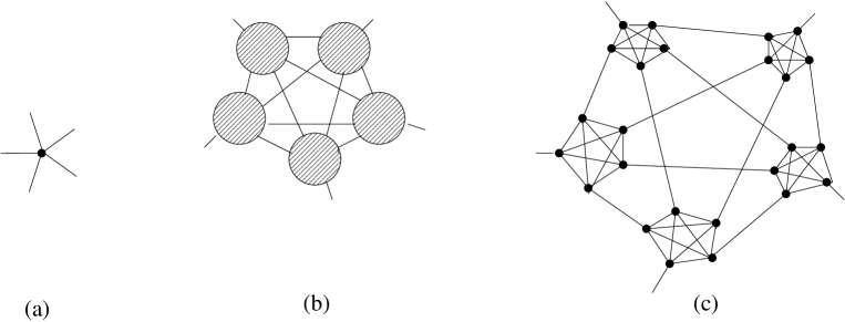
Figure 2: The recursive construction of the $n$-simplex fractal for $n=5$. (a) The first order graph (b) the graph of a $(r+1)$ order triangle, formed by joining $n$ $r$-th order graphs, shown as shaded blobs here (c) the second order graph.

The first family we shall discuss is the $n$-simplex family, defined for all positive integers $n>2$. The $n=3$ case was first defined by Nelson and Fisher [11], who called it truncated tetrahedron lattice. The construction was generalized for arbitrary $n$ in [12]. The recursive construction of the graph of the fractal is shown in Fig. 2. The first order graph is a single vertex with $n$ bonds. In general, the $r$-th order graph will have $n^{r-1}$ vertices, and $(n^{r}+n)/2$ bonds. Of these $(n^{r}-n)/2$ are internal bonds, and there are $n$ external bonds, that are used to connect this graph to other vertices to form bigger graphs. To form a graph of $(r+1)$-th order, we take $n$ graphs of $r$-th order, and join them to each other by connecting a dangling bond of each to a dangling bond of the other $r$-order subgraphs. There is one dangling bond left in each of the subgraphs, and $n$ bonds altogether. These form the dangling bonds of the $(r+1)$-th order graph. We let $r$ tend to infinity to get an infinite graph. The fractal dimension $D_{n}$ of this graph is easily seen to be $\log n/\log 2$. It was shown in [12] that the spectral dimension ${\tilde{d}}_{n}$ of this graph is $2\log n/\log(n+2)$.

The second family we shall consider is the Given-Mandelbrot family of fractals [13], defined in Fig. 3. Members of the family are characterized by an integer $b$, with $2\leq b<\infty$. We start with a graph with three vertices and three edges forming a triangle. This is called the first order triangle. To construct the graph of the $(r+1)$-th order triangle, we join together graphs of $b(b+1)/2$ triangles of $r$-th order, (i.e. identify corner vertices) as shown in the figure, to form an equilateral triangle with base which is $b$ times longer. We shall call the resulting graph the $GM_{b}$ fractal.

It is easy to see that the number of edges in the graph of the $r$-th order triangle is
$3[b(b+1)/2]^{r-1}$. The fractal dimension is $D_{b}={\log}[b(b+1)/2]/\log b$. For $b=2,3,4..$, these values are $1.5849,1.6309,1.6609...$ respectively. The spectral dimension $\tilde{d}_{b}$ of the graph can also be calculated exactly for general $b$ [14]. The values of ${\tilde{d}_{b}}$ for $b=2$ to $10$ are listed in [15]. For large $b$, $\tilde{d}_{b}$ tends to $2$, and the leading correction to its limiting value is given by $\tilde{d}_{b}\approx 2-\log\log b/\log b$ [16].

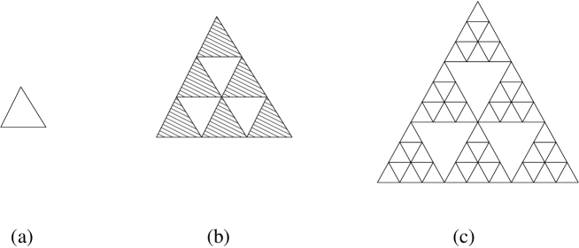
Figure 3: The recursive construction of the Given-Mandelbrot fractal for $b=3$. (a) The graph of first order triangle.(b) the graph of a $(r+1)$ order triangle, formed by joining $b(b+1)/2$ $r$-th order triangles shown as shaded triangles here (c) graph of the $2$nd order triangle.

In fact, following Hilfer and Blumen [15], one can define a general fractal family of Sierpinski -like fractals, to be called $HB(b,d)$ family here, such that the the $n$-simplex corresponds to $HB(2,n-1)$, and the $GM_{b}$ fractal corresponds to $HB(b,2)$. Here the basic unit is a $(d+1)$-simplex graph, and one makes the $(r+1)$-th order graph by making a simplex of $b$ layers of the $r$-th order graphs. The construction is illustrated in Fig. 4 for the fractal $HB(3,3)$.

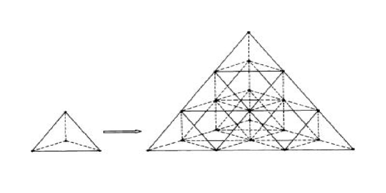
Figure 4: First two stages in the iterative construction of the Hilfer-Blumen fractal $HB(3,3)$. This has a fractal dimension ${\bar{d}}=\log 10/\log 3.$

The third family of fractals we shall use is a generalization of the modified rectangular lattice [12]. Here the first order graph is a set of $2^{d}$ vertices forming a $d$-dimensional hypercube. In general, the $r$-th order graph has $2^{r+d-1}$ vertices in the shape of a cuboid, with each corner vertex of the cuboid having an extra dangling bond to connect to outside. The graph of an $(r+1)$-th order cuboid is formed by taking two $r$-th order cuboids, and joining the opposite faces by $2^{d-1}$ bonds. The direction of the face that is selected for this is changed cyclically at the next order, so that the lengths of different sides of the cuboid are within a factor 2 of each other. It is easily seen that the fractal dimension of this graph is $d$, and it can be shown that the spectral dimension is $2(1-2^{-d})$. The construction is illustrated in Fig. 5 for the case $d=2$.

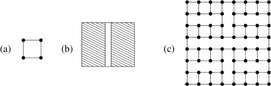
Figure 5: The recursive construction of the modified rectangular lattice for $d=2$. (a) The graph of first order square.(b) the $(r+1)$-th order graph, formed by joining $2$ $r$-th order graphs shown as shaded rectangles here (c) graph of the $5$th order rectangle.

The determination of the generating function for the linear polymers on these fractals follows the treatment of [17, 18]. Let $P_{n}(N)$ be the number of distinct simple polygons of perimeter $n$ on a graph with $N$ total number of sites in the graph, different translations of the polymer being counted as distinct. [The use of same symbol $n$ for the $n$-simplex and $n$-stepped walk should not cause any confusion, as it is clear from context which is intended.] For large $N$, this number increases linearly with $N$. We then define ${\bar{P}}_{n}$ as the average number of polygons of perimeter $n$ per site by

$$\bar{P_{n}}=Lim_{N\rightarrow\infty}\frac{P_{n}(N)}{N};$$ (1)

and

$$P(x)=\sum_{n=3}^{\infty}{\bar{P}}_{n}x^{n},$$ (2)

For large $n$, ${\bar{P}_{n}}$ varies as $\mu^{n}n^{\alpha-3}$, where $\mu$ is a constant, and $\alpha$ is a critical exponent for the walks. This corresponds to $P(x)\sim(1-\mu x)^{2-\alpha}$, for $x$ tending to $1/\mu$ from below. Note that $P(x)$ is a finite-degree polynomial in $x$ for the graphs like the Husimi cactus (Fig. 1).

We similarly define ${\bar{C}_{n}}$, the average number of open walks of length $n$, as the average over all positions of the root, of the number of $n$-stepped self-avoiding walks. For large $n$, this varies as $\mu^{n}n^{\gamma-1}$, which defines the critical exponent $\gamma$. The corresponding generating function

$$C(x)=\sum_{n=1}^{\infty}{\bar{C}_{n}}x^{n}$$ (3)

varies as $(1-x\mu)^{-\gamma}$ as $x$ tends to $1/\mu$ from below. We also define the critical exponent $\nu$ for SAWs by the relation that the average end-to-end distance for walks of length $n$ varies as $n^{\nu}$ for large $n$.

Here in the context of disordered systems, we imagine that the polymer can freely move over all space, and the averages calculated correspond to annealed averages, as we are averaging the partition function of SAWs over different positions of the root. The logarithm of the number of polymer configurations is the entropy, and one can also define the equivalent of quenched averages, where one averages, not the numbers of walks, but logarithms of numbers of rooted walks, over different positions of the root. These are more difficult to determine. We will indicate how these can be handled in sec. 3.

3 RENORMALIZATION EQUATIONS FOR THE $3$-SIMPLEX FRACTAL

The procedure to determine the critical behavior of SAWs on fractals is simplest to illustrate using the $3$-simplex as an example. We will keep the presentation informal (hopefully not inaccurate). Readers who prefer a more formal approach, may consult [19]. We discuss the calculation of annealed averages first.

3.1 Calculation of annealed averages

Consider one $r$-th order triangular subgraph of the infinite order graph. It is connected to the rest of the lattice by only three bonds. Our aim to sum over different configurations of the SAW on this subgraph, with a weight $x$ for each step of the walk. These can be divided into four classes, as shown in Fig. 6. Here $A^{(r)}$ is the sum over all configurations of the walk within the $r$-th order triangle, that enters the triangle from a specified corner, and with one endpoint inside the triangle. $B^{(r)}$ is the sum over all configurations of walk within the triangle that enters and leaves the triangle from specified corners. In $C^{(r)}$, the walk enters and leaves the subgraph from specified vertices, and reenters afterwards from the third corner, and has one endpoint inside the triangle. $D^{(r)}$ consists of sum over configurations that have both endpoints of the walk inside the triangle, but part of the walk is outside the triangle. We can write down the values of these for $r=1$ immediately.

$$A^{(1)}=\sqrt{x},~{}B^{(1)}=x,~{}C^{(1)}=~{}D^{(1)}=0.$$ (4)

We define the order of a closed polygon on the infinite $3$-simplex graph to be $r$, if the polygon is completely contained inside an $r$-th order triangle, but not inside any $(r-1)$-th order triangle. It is easy to see that sum over all $r$-th order polygons within one such triangle is ${B^{(r-1)}}^{3}$. The number of sites in the $(r+1)$-th order triangle is $3^{r}$, hence we get

$$P(x)=\sum_{r=1}^{\infty}3^{-r}{B^{(r)}}^{3}.$$ (5)

The sum over open walks can be expressed similarly

$$C(x)=\sum_{r=1}^{\infty}3^{-r}[3{A^{(r)}}^{2}+3B^{(r)}{A^{(r)}}^{2}+3{B^{(r)}}^{2}D^{(r)}].$$ (6)

It is straight forward to write down the recursion equations for these weights $A^{(r+1)},B^{(r+1)},$ $C^{(r+1)}$ and $D^{(r+1)}$ in terms of the values at order $r$. For example, Fig. 7 shows the only two possible ways one can construct a polymer configuration of type $B$. It is easy to verify that the resulting equations are [17]

$$A^{(r+1)}=A(1+2B+2B^{2})+C(2B^{2});$$ (7)

$$B^{(r+1)}=B^{2}+B^{3};$$ (8)

$$C^{(r+1)}=AB^{2}+C(3B^{2});$$ (9)

$$D^{(r+1)}=(A^{2}+2A^{2}B+4ABC+6BC^{2})+D(2B+3B^{2});$$ (10)

where we have dropped the superscripts $(r)$ in the right-hand side of the equations to simplify notation.

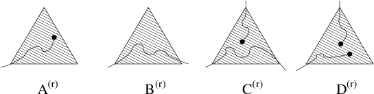
Figure 6: Restricted partition functions for the $3$-simplex lattice.

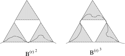
Figure 7: Graphical representation of terms that contribute to the recursion equation for $B^{(r+1)}$ for the $3$-simplex lattice.

It is straightforward to determine the analytical behavior of the generating functions $P(x)$ and $C(x)$ from the equations (4)-(10).

We note that the equation for $B^{(r+1)}$ depends only on $B^{(r)}$, and does not involve the other variables. The recursion equation (8) has two trivial fixed points $B^{*}=0$, and $B^{*}=\infty$, and a non-trivial fixed point $B^{*}$ given by $B^{*}=(\sqrt{5}-1)/2$. For $B^{(0)}=x<B^{*}$, the variables $B^{(r)}$ decrease with $r$ under iteration, and tend to zero for large $r$. For $B^{(0)}>B^{*}$, $B^{(r)}$ increases with $r$, and diverges to infinity, and the series for $P(x)$ and $C(x)$ diverge. This implies that

$$x_{c}=B^{*}=1/\mu=[\sqrt{5}-1]/2.$$ (11)

which shows that the growth constant $\mu$ of SAWs on this lattice is the golden mean.

Using Eq. (8), we see that $P(x)$ satisfies the functional equation

$$P(x)=\frac{x^{3}}{3}+\frac{1}{3}P(x^{2}+x^{3}).$$ (12)

From this equation, we get $P(x=B^{*})=\mu^{-3}/2$. For $x$ near $B^{*}$, we can linearize the recursion equation. We write $x=B^{*}-\delta$, and $Q(\delta)=P(B^{*})-P(B^{*}-\delta)$ giving

$$Q(\delta)\approx\mu^{-2}\delta+\frac{1}{3}Q((2+\mu^{-2})\delta).$$ (13)

If we assume that the singular part of $Q(\delta)$ varies as $\delta^{2-\alpha}$, this gives us

$$\alpha=2-\frac{\log 3}{\log(2+\mu^{-2})}\simeq 0.7342.$$ (14)

Figure 8: Plot of the difference between the exact value of $\log{\bar{P}}_{n}$ and the asymptotic form showing log-periodic oscillations with $n$ for the $3$-simplex lattice.

The recursion equations for $A^{(r+1)}$ and $C^{(r+1)}$ are linear in $A^{(r)}$ and $C^{(r)}$, with coefficients that depend on $B^{(r)}$. If we start with a value $\delta\ll 1$, then there is a value $r_{0}$, such that for $r-r_{0}\ll-1$, we can assume $B^{(r)}\simeq B^{*}$, and for $r-r_{0}\gg 1$, $B^{(r)}\simeq 0$. As

$$B^{(r+1)}-B^{*}\simeq(2+\mu^{-2})(B^{(r)}-B^{*}),$$ (15)

we have clearly

$$r_{0}=\frac{\log(1/\delta)}{\log(2+\mu^{-2})}.$$ (16)

For $r<r_{0}$, in the recursion equations for $A^{(r)}$ and $C^{(r)}$, we can put $B^{(r)}=B^{*}$, giving

$$\left(\begin{array}[]{ll}A^{(r+1)}\\ C^{(r+1)}\end{array}\right)=\left(\begin{array}[]{lrlr}~{}~{}1+2\mu^{-1}+2\mu^{-2}&2\mu^{-2}\\ ~{}~{}\mu^{-2}&3\mu^{-2}\end{array}\right)\left(\begin{array}[]{ll}A^{(r)}\\ C^{(r)}\end{array}\right).$$ (17)

This implies that $A^{(r)}$ and $C^{(r)}$ vary as $\lambda_{+}^{r}$, where $\lambda_{+}$ is the larger eigenvalue of the $2\times 2$ matrix in Eq. (17). For $r>r_{0}$, $A^{(r)}\simeq A^{(r_{0})}$, and $C^{(r)}\simeq 0$, then, in Eq. (6), the leading contribution comes from the term $r=r_{0}$, giving

$$C(x=x_{c}-\delta)\simeq(\frac{\lambda_{+}^{2}}{3})^{r_{{}_{0}}}\sim(1/\delta)^{-\gamma},$$ (18)

with

$$\gamma=\frac{\log(\lambda_{+}^{2}/3)}{\log(2+\mu^{-2})}\simeq 1.3752.$$ (19)

The typical size of the polymer for $x=x_{c}-\delta$ is $2^{r_{{}_{0}}}$, which varies as $(1/\delta)^{\nu}$, with

$$\nu=\frac{\log 2}{\log(2+\mu^{-2})}\simeq 0.7986.$$ (20)

It is quite straightforward to generate the exact series $P(x)$ using Eq.(5) with symbolic manipulation programs like Mathematica. Just keeping terms up to $r=7$, we get a series for $P(x)$ exact up to $x^{383}$ ( the coefficient of this term has more than 70 digits!). As seen above, the singular part of $P(x)$ varies as $(1-x^{\mu})^{2-\alpha}$ for $x$ near $\mu^{-1}$ its $n^{th}$ Taylor coefficient must vary as $\mu^{n}n^{\alpha-3}$. However, in general, the solution of Eq.(13) allows an additive term which is periodic function of $\log\delta$ with period $\log(2+\mu^{-2})$. In Fig. 8, we have plotted the difference $\Delta\log P_{n}$ between the exact value of $\log{\bar{P}}_{n}$ and the asymptotic value $\log(\mu^{n}n^{\alpha-3})$. We clearly see the log-periodic oscillations. Such log-periodic oscillations are seen in many other systems showing discrete scale-invariance [20]. The existence of these oscillations makes it very difficult to estimate critical exponents from extraplations of exact series expansions using only a few terms [21].

For the fugacity $x>x_{c}$, the linear polymer fills the available space with finite density. Since the logarithm of the single loop partition function for the $r$-th order triangle is now proportional to the number of sites in the triangle, we define the free energy per site in the dense phase as

$$f(x)=\lim_{r\rightarrow\infty}\frac{\log B^{(r)}}{3^{r-1}}.$$ (21)

Then, from Eq.(8), it follows that $f(x)$ satisfies the equation

$$f(x)=\frac{1}{3}f(x^{2}+x^{3}).$$ (22)

The density of the polymer $\rho(x)$ in the dense phase is given by

$$\rho(x)=x\frac{d}{dx}f(x)=\frac{2+3x}{3(x+1)}\rho(x^{2}+x^{3}).$$ (23)

Iterating this equation, we get

$$\rho(x)=\prod_{r=1}^{\infty}[(B^{(r)}+\frac{2}{3})(B^{(r)}+1)^{-1}].$$ (24)

From Eq. (22), it can be seen that as $x$ tends to $x_{c}$ from above, the polymer density decreases as $(x-x_{c})^{1-\alpha}$. Equivalently, for small densities $\rho$, the entropy per monomer $\mu(\rho)\simeq\mu(0)-K\rho^{\frac{1}{1-\alpha}}$, where $K$ is some constant.

3.2 Quenched averages

We note that the $3$-simplex lattice is not homogenous, and different sites are not equivalent. In the context of disordered systems, the calculation of $P(x)$ and $C(x)$ are examples of annealed averages. We now show how one can calculate “quenched averages” in this problem.

We define $P_{n}(S)$ as the number of polygons of perimeter $n$ that pass through a given site $S$ ( these are called rooted polygons, one could also study rooted open walks), and ask how does it vary with $S$. What is its average value, variance etcetra ? A quantity of particular interest is the average value of $\log P_{n}(S)$. A good understanding of these for the regular fractals is prerequisite for understanding the more complicated case of random quenched disorder. We mention briefly some very recent results about the behavior of fluctuations of $P_{n}(S)$ with $S$ [22].

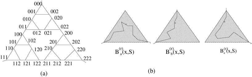
Figure 9: (a) labelling of different sites on the $3$-simplex (b) definition of weights for rooted graphs

To describe rooted polygons, we first need to set up a coordinate system to describe different sites on the fractal. A simple and natural choice for this is shown in fig. 9. A point on the $r$-th order triangle is labelled by a string of $(r-1)$ characters, e.g. $0122201\ldots$. Each character takes one of three values $0,1$ or $2$. The leftmost character specifies in which of the three sub-triangles the point lies ($0$, $1$ and $2$ for the top, left and right subtriangle respectively). The next character specifies placement in the $(r-1)$-order sub-triangle, and so on. The restricted partition functions for the rooted polygons are also defined in 9. Here $B^{(r)}_{a}(x,S)$ is the sum over walks on the $r$-th order triangle that go through the left and right corners of the triangle, and also visit the site characterized by string $S$ inside the triangle. Other weights are defined similarly.

Figure 10: A plot of the average value of $\log P_{n}(S)\mu^{-n}$ as a function of $n$. The uppermost and the lowermost curves are theoretically derived upper and lower bounds to this number over different positions of the root. The dashed and dotted lines show the annealed and quenched average values respectively.

A site in the $(r+1)$-th order will be characterized by a string of $r$ characters. Hence, a site characterized by string $S$ at the $r$-th stage will be characterized by one of the strings $0S$, $1S$ or $2S$. The recursion relations in this case are linear, and can be written in the matrix form

$$\left(\begin{array}[]{ll}B^{(r+1)}_{a}(x,sS)\\ B^{(r+1)}_{b}(x,sS)\\ B^{(r+1)}_{c}(x,sS)\\ \end{array}\right)={\cal{M}}_{s}\left(\begin{array}[]{ll}B^{(r)}_{a}(x,S)\\ B^{(r)}_{b}(x,S)\\ B^{(r)}_{c}(x,S)\\ \end{array}\right),$$ (25)

where

$${\cal{M}}_{0}=\left(\begin{array}[]{lll}B^{2}~{}~{}0~{}~{}0\\ ~{}0~{}~{}B~{}~{}B^{2}\\ ~{}0~{}~{}B^{2}~{}B\\ \end{array}\right);~{}~{}{\cal{M}}_{1}=\left(\begin{array}[]{lll}~{}B~{}~{}0~{}B^{2}\\ ~{}~{}0~{}B^{2}~{}0\\ ~{}B^{2}~{}0~{}~{}B\\ \end{array}\right);~{}~{}{\cal{M}}_{2}=\left(\begin{array}[]{lll}B~{}B^{2}~{}0\\ B^{2}~{}B~{}0\\ ~{}0~{}~{}0~{}B^{2}\\ \end{array}\right),$$ (26)

and we have suppressed the superscript $(r)$ on $B$ in the matrices. The generating function for rooted polygons is given by

$$P(x,S)=\sum_{r=1}^{\infty}B^{(r)}_{a}(x,S_{r}){B^{(r)}}^{2},$$ (27)

where $S_{r}$ is the string consisting of the last $(r-1)$ characters of the position of $S$. If we ignore the constraint that the walk has to pass through $S$, we get an upper bound on the number of such walks, $B^{(r)}_{a}(x,S)\leq B^{(r)}(x)$, where inequality between polynomials is understood to imply inequality for the coefficient of each power of $x$. This implies that for all sites $S$,

$$P(x,S)\leq\sum_{r=0}^{\infty}{B^{(r)}}^{3}.$$ (28)

If we write the right-hand-side as ${\cal F}_{u}(x)$, then ${\cal F}_{u}(x)$ satisfies the equation

$${\cal F}_{u}(x)=x^{3}+{\cal F}_{u}(x^{2}+x^{3}).$$ (29)

This equation should be compared with Eq.(13), and differs from it only in the absence of the factor $1/3$. This functional equation has the fixed point at $x^{*}=1/\mu$, and linear analysis near the fixed point shows that ${\cal F}_{u}(x)$ diverges as $-\log(1-x\mu)$ for $x$ tending to $1/\mu$ from below. This implies that the coefficient of $x^{n}$ in the Taylor expansion of ${\cal F}_{u}$ varies as $\mu^{n}/n$ for large $n$. Thus,

$$P_{n}(S)\leq K\mu^{n}/n,{\rm~{}~{}for~{}all}~{}n,{\rm~{}and~{}all}~{}S,$$ (30)

where $K$ is some constant. Sumedha and Dhar [22] also derive a lower bound $P_{n}(S)\geq K_{1}\mu^{n}n^{-b-1}$, for all $n$ and all $S$, where $b=2\log\mu/\log(2+\mu^{-2})\simeq 0.92717$, and $K_{1}$ is some constant. For a randomly chosen $S$, the problem reduces to a random product of noncommuting matrices ${\cal M}_{0}$, ${\cal M}_{1}$ and ${\cal M}_{2}$. The expected value of the logarithm of a product of $r$ independent random matrices varies linearly with $r$ for large $r$. This implies that for large $n$, the quenched average $<\log P_{n}(S)>$ varies as $n\log\mu-(2-\alpha_{q})\log n$. The numerical estimate of $\alpha_{q}$ is approximately $0.729\pm.001$, which is just a bit less than the annealed value $0.7342$. In figure 10, we have plotted the numerical values of the upper and lower bounds to $\log(P_{n}(S)\mu^{-n})$, and the annealed and quenched averages $\log<P_{n}(S)\mu^{-n}>$, and $<\log(P_{n}(S)\mu^{-n})>$. It should be noted that the lower bound is the best possible, in the sense that for each value of $n$, there is a finite density of roots that saturate the bound. The upper bound is not always optimal. Also, whether the annealed and quenched averages are very close or less so appears to be an oscillatory function of $\log n$.

4 RECURSION EQUATIONS FOR OTHER FRACTALS

We now briefly indicate how the real-space renormalization group technique of the previous section can be extended to other fractals.

4.1 $n$-simplex fractals for $n>3$

The case of $n$-simplex fractal for higher $n$ is a straight forward extension of the technique used for the $3$-simplex. The case $n=4$ was studied in [17], and the treatment was extended to $n=5$ and $6$ in [23].

For higher $n$, the number of restricted partition functions we have to define to generate a closed set of recursion equations is larger. Here the permutation symmetry between the corner vertices of the $n$-simplex graph is very useful in reducing the number of variables needed. For $n=4$ and $5$, we need two functions $A^{(r)}$ and $B^{(r)}$ to generate the closed loops generating function $P(x)$. For the open walks generating function $C(x)$, four more variables are needed. Their definition is shown in Fig. 11. They will be denoted by $C^{(r)},D^{(r)},E^{(r)}$ and $F^{(r)}$.

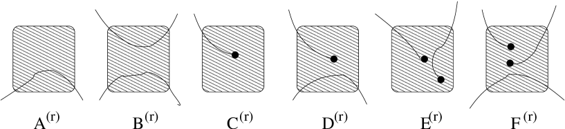
Figure 11: Different restricted partition functions for the $4$-simplex lattice. The shaded squares denote graphs of $r$-th order $4$-simplex, of which only the external bonds are shown.

The starting values of these weights are

$$A^{(1)}=x;\hskip 56.9055ptC^{(1)}=\sqrt{x};\hskip 56.9055ptB^{(1)}=D^{(1)}=E^{(1)}=F^{(1)}=0.$$ (31)

The recursion relations for these weights are written by constructing graphs by all possible ways. This leads to [17]

$$A^{(r+1)}=A^{2}+2A^{3}+2A^{4}+4A^{3}B+6A^{2}B^{2},$$ (32)

$$B^{(r+1)}=A^{4}+4A^{3}B+22B^{4},$$ (33)

and similar equations for the other variables (omitted here). The expression for $P(x)$ in this case is

$$P(x)=\sum_{r=1}^{\infty}(4{A^{(r)}}^{3}+3{A^{(r)}}^{4}).$$ (34)

There is a similar but more complicated expression for the generating function for open walks. We note that recursions of $A^{(r+1)}$ and $B^{(r+1)}$ depend only on $A^{(r)}$ and $B^{(r)}$. For any given value of $x$, we can determine $P(x)$ numerically by explicitly iterating the recursion equations. One finds

$$x_{c}=0.4373,\qquad\mu=2.2866,$$ (35)

and the corresponding non-trivial fixed point is $(A^{*},B^{*})=(0.4264,0.04998)$. Linearization of Eqs. (32) and (33) around this fixed point gives largest eigenvalue $\lambda_{1}=2.7965$. We can express the end-to-end distance exponent $\nu$ in terms of $\lambda_{1}$ using arguments similar to the case of 3-simplex. We get

$$\nu=\frac{\log 2}{\log\lambda_{1}}=0.6740,$$ (36)

and specific heat exponent

$$\alpha=2-\nu D_{4}=0.6519.$$ (37)

To find $\gamma$, we consider the recursion equations for $C^{(r+1)}$ and $D^{(r+1)}$, which are linear in $C^{(r)}$ and $D^{(r)}$, and diagonalizing the $2\times 2$ matrix gives the eigenvalue $\lambda_{+}=4.2069$, which corresponds to $\gamma=\log[(\lambda_{+}^{2})/4]/\log[\lambda_{1}]=1.4461$.

For the $5$-simplex lattice, the closed loop generating function can be found in terms of variables $A^{(r)}$ and $B^{(r)}$, defined as before. In this case, the recursion equations are more complicated [23]. We list these here to show how the complexity of the polynomials rises rapidly with increasing $n$:

$$A^{(r+1)}=132(B^{5}+AB^{4})+A^{2}(1+18B^{2}+96B^{3})+A^{3}(3+12B+78B^{2})+A^{4}(6+30B)+6A^{5},$$ (38)

$$B^{(r+1)}=186B^{5}+220AB^{4}+88A^{2}B^{3}+A^{4}(1+13B+220B^{4})+2A^{5}.$$ (39)

We omit the other equations. Starting with $(A^{(1)},B^{(1)})=(x,0)$, one finds a non-trivial fixed point for $x=x_{c}=0.336017$, which corresponds to $\mu=1/x_{c}=2.97603$ and the fixed point $(A^{*},B^{*})=(0.3265,0.02791)$. Linearization of the recursion relations Eq. (38) and (39) around this fixed point leads to one eigenvalue $\lambda_{1}=3.13199$ greater than unity. Using this value of $\lambda_{1}$ one gets $\nu=0.6049$ and $\alpha=0.5955$.

The exponent $\gamma$ is found from the recursion relations for the variables corresponding to a single end point. The largest eigenvalue $\lambda_{+}$ of the matrix which characterizes the linear transformation of the recursion relations of these functions is $\lambda_{+}=5.24398$ corresponding to $\gamma=1.4875$.

For the $6$-simplex lattice, even for the polygon generating function, we need three restricted partition functions $A^{(r)},B^{(r)}$ and $C^{(r)}$, corresponding the cases where the walk enters and exits the $r$-th order subgraph once, twice or three times respectively. For the open walks, we need six more variables. For details, consult [23]. In this case, the nontivial fixed point is found to be

$$(A^{*},B^{*},C^{*})=(0.262352,0.017588,0.0007011).$$ (40)

This fixed point is reached if we start with $x=x_{c}=0.27166$, which corresponds to the connectivity constant $\mu=3.68107$. The linearization of recursion relations about this fixed point yields only one eigenvalue, $\lambda_{1}=3.4965$, higher than unity giving $\nu=0.5537$ and $\alpha=0.5686$.

By diagonalizing the matrix corresponding to the linear recursions for weights corresponding to one end point, one gets the largest eigenvalue $\lambda_{+}=6.26709$. This gives $\gamma=1.500094$ for the $6$-simplex lattice.

4.2 $n$-simplex lattice in the limit of large $n$

One can explicitly determine the critical exponents for a few more values of $n$ using a computer to generate the recursion equations. However, this soon becomes very time-consuming. If $n$ is very large, some simplifications occur, and one can determine the leading behavior of the critical exponents of the SAW problem on the $n$-simplex in this limit [24]. We discuss this below.

We start by noting that as $n$ increases, the probability of occurrence of loops in a random walk on the graph decreases, and as the loops become rarer, the random walk without self-exclusion should approximate the properties of the SAW. In particular, we would expect that the growth constant for SAWs on the $n$-simplex should be approximately equal to $n-1$. Let us denote, as before, the restricted partition functions for the $r$-th order lattice corresponding to polygon generating function by $A^{(r)},B^{(r)},C^{(r)}\dots$, corresponding to configurations where the SAW enters (and exits) the graph once, twice, thrice $\ldots$respectively. Then for the fixed point corresponding to the swollen state, we would have $A^{*}\sim{1}/{n}$. Since $B^{(r)}\leq{A^{(r)}}^{2}$, it is at most of order ${1}/{n^{2}}$, and similarly, $C^{*}$ is at most of order ${1}/{n^{3}}$. Thus, $B^{*},C^{*},.....$ approach zero faster than $A^{*}$ as $n$ is increased.

It is straight forward to write down the recursion equation for $A^{(r+1)}$ if we neglect the terms involving $B,C,$ etc. There is only one configuration of walk corresponding to the term $A^{2}$ ( we drop the superscript of $A^{(r)}$ for convenience), but $(n-2)$ terms of type $A^{3}$, and $(n-2)(n-3)$ terms of type $A^{4}$ etc. This gives us the recursion equation

$$A^{(r+1)}\simeq A^{2}+(n-2)A^{3}+(n-2)(n-3)A^{4}+.......+(n-2)!A^{n}.$$ (41)

When $A$ is of order $1/n$, each of these terms is of order $1/n^{2}$, and the sum needs to be evaluated with some care. In [23], it was noted that, with only a small error when $A$ is near $A^{*}$, this series can be rewritten as

$$A^{(r+1)} \simeq A^{n}(n-2)![1+1.A^{-1}+(1/2!)A^{-2}+\dots+(1/(n-2)!)A^{-n+2}]$$ (42)

$$\simeq (n-2)!~{}A^{n}~{}\exp(1/A)$$ (43)

One can then study the asymptotic behavior of this recursion equation for large $n$. Here we shall use a different approach. If we change the variable from $A^{(r)}$ to $\epsilon^{(r)}$ using the relation

$$A^{(r)}=\frac{1}{n}\exp(\frac{\epsilon^{(r)}}{\sqrt{n}}).$$ (44)

and use the fact that, for $n\gg r\gg 1$,

$$\prod_{j=1}^{r}(1-j/n)\simeq\exp(-\frac{r^{2}}{2n}),$$ (45)

the series of Eq.(35) can be written as

$$A^{(r+1)}\simeq(\frac{1}{n^{2}})\sum_{r=2}^{n}\exp(\frac{\epsilon^{(r)}r}{\sqrt{n}}-\frac{r^{2}}{2n}).$$ (46)

Substituting $x$ for $r/\sqrt{n}$ and replacing the summation over $r$ for $\sqrt{n}\gg\epsilon^{(r)}\gg 1$ by integration over $x$ from $-\infty$ to $\infty$ (for $\epsilon\gg 1$, the lower limit can be extended to $-\infty$ with negligible error) we get

$$A^{(r+1)}\simeq(\frac{\sqrt{2\pi}}{n^{3/2}})\exp(\frac{{\epsilon^{(r)}}^{2}}{2}).$$ (47)

From this equation, we see that the nontrivial fixed point is given by

$$\epsilon^{(r)}=\epsilon^{*}\approx\sqrt{\log n}.$$ (48)

Let us now look at the equation for $B^{(r+1)}$. Again keeping only the terms involving $A$’s alone, we get

$$B^{(r+1)}\simeq A^{4}+2(n-4)A^{5}+3(n-4)(n-5)A^{6}+\ldots$$ (49)

Using the same approximation as before, we get

$$B^{(r+1)}\simeq(\frac{1}{n^{4}})\sum_{r=1}^{n}r\exp(\frac{\epsilon r}{\sqrt{n}}-\frac{r^{2}}{2n})\simeq\frac{\sqrt{2\pi\log n}}{n^{5/2}},$$ (50)

where we have used the approximate fixed point value of $\epsilon^{*}$ from Eq.(48). The fact that $B^{(r+1)}$ decreases faster than $n^{-2}$ justifies neglecting these terms in determining the asymptotic behavior of the recursions. The value of the derivative of the linearized recursion equation for $A$ at the nontrivial fixed point is

$$\frac{d}{dA}A^{(r+1)}\simeq\sqrt{n\log n}.$$ (51)

This implies that the critical exponent $\nu$ is given by

$$\nu\simeq\frac{2\log 2}{\log n}\left[1-\frac{\log\log n}{\log n}+{\rm higher~{}~{}order~{}~{}terms}\right].$$ (52)

We note that the correction term to Eq.(41) involving $B^{(r)}$ in leading order are of the form

$$\Delta A^{(r+1)}=2A^{3}B(n-2)(n-3)+4A^{4}B(n-2)(n-3)(n-4)+....$$ (53)

Using the estimate Eq.(50) for $B^{(r)}$, we see that near the fixed point, the error in Eq.(41) $\Delta A^{(r+1)}$ is of order $n^{-3/2}$. This implies that the fractional error in the value of $\nu$ using Eq.(41) is of order $n^{-1/2}$. Thus Eq.(41) is much more accurate than Eq.(52), where the error is of order $1/(\log n)$.

To calculate $\gamma$, one has to consider configurations with one endpoint of walk inside the graph. Again, keeping only terms involving powers of $A$, the recursion relation for the weight of configurations with the walk entering the graph once ( call it $X$) is found to be

$$X^{(r+1)}\simeq X[1+(n-1)A^{*}+(n-1)(n-2)A^{*2}+....+(n-1)!A^{*(n-1)}].$$ (54)

Using the arguments as before, this can be evaluated using the fixed point value of $A^{*}$, giving

$$X^{(r+1)}\simeq X\sqrt{n\log n}.$$ (55)

It follows that, for large $n$,

$$\gamma\simeq 2\left[1-\frac{\log\log n}{\log n}+{\rm~{}higher~{}order~{}terms}\right].$$ (56)

Note that the critical exponents do not take mean-field values, even when the fractal dimension of the lattice becomes greater than $4$. This is clearly because of the special structure of the $n$-simplex lattice, where, even though the fractal dimension becomes greater than $4$ for large $n$, the spectral dimension remains below $2$, and probability of intersection of paths of random walks remains large. Also that the non-analytical dependence of the type $\frac{\log\log n}{\log n}$ in the critical exponents on the lattice cannot be obtained from $\epsilon$-expansion like power-series expansions in deviation of dimensionality from some reference value.

4.3 Modified rectangular lattice

This lattice is interesting as its fractal dimension, and the spectral dimension are both rational numbers. Also, one can get its graph by selectively deleting some bonds from the graph of $d$-dimensional hypercubical lattice. Since the $(r+1)$-th order graph is formed by taking only two smaller graphs, the recursion equations involve only a small number of configurations, and are easy to write down. But the number of variables needed is larger, as the symmetry of the graph is lower than that of the $HB(b,d)$ family.

The behavior of SAWs on the $d=2$ lattice was studied in [17]. The recursion equation for a polygon is written in terms of five restricted generating functions (see Fig. 12) by constructing graphs by all possible ways [17]. This gives

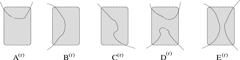
Figure 12: Diagrams representing the restricted partition functions for the various ways the polymer can cross the r^th order rectangle.

$$A^{(r+1)} = B(1+D),\qquad B^{(r+1)}=A^{2}+C^{2},\qquad C^{(r+1)}=2AC,$$

$$D^{(r+1)} = B^{2}+2DE,\qquad E^{(r+1)}=D^{2}.$$ (57)

The starting values of these recursions are

$$A^{(1)} = B^{(1)}=x^{2}+x^{4},\qquad C^{(1)}=2x^{3},\qquad D^{(1)}=E^{(1)}=x^{4}.$$ (58)

The polygon number generating function $P(x)$ is given by [17]

$$P(x)=\frac{x^{4}}{4}+\sum_{r=1}^{\infty}[\frac{(B^{(r)})^{2}}{2^{r+2}}].$$ (59)

Numerical iteration of these equations gives $x_{c}=0.5914$ and $\mu=1.6909$. The fixed point occurs at

$$(A^{*},B^{*},C^{*},D^{*},E^{*})=(0.5000,0.4201,0.4124,0.1902,0.0362),$$ (60)

giving one eigenvalue $\lambda_{1}=1.6839$ greater than one. Using this eigenvalue one finds $\nu=\log 2/2\log\lambda_{1}=0.66503\;{\rm and}\;\alpha=0.6699$. A similar analysis for the open-walk configurations gives the critical exponent $\gamma=1.4403$.

5 SELF-AVOIDING WALKS ON FRACTALS WITH DIMENSION $2-\epsilon$

In the preceding sections we studied the properties of SAWs on several different fractals. For the calculation of critical exponents of SAWs on still other fractals, see for example [25]. It would appear that for each fractal, one has to write down the polynomial recursion equations, and calculate the values of critical exponents using the technique outlined. There is no simple expresion for the critical exponents as a function of the geometrical properties of the fractal, ( an improved Flory formula?) that would allow one to predict these without doing the full calculation. Unfortunately, this level of understanding of the problem is still not achieved.

The best way to understand such systematics is to study the variation of exponents across a family of fractals as some property of the fractal is changed. For the $n$-simplex family studied earlier, the fractal and spectral dimensions did not tend to the same value for large $n$. We now discuss variation of critical exponents for SAWs on the $GM_{b}$ fractals family as the parameter $b$ is varied from $2$ to infinity. For large $b$, both the fractal and spectral dimensions of the fractal tend to $2$ where the properties of walks are well-understood. Such a study makes contact with the formal $\epsilon$-expansion technique which has played an important role in development of renormalization theory of critical phenomena.

The self-avoiding walks for the $GM_{2}$ fractal have the same exponents as for the $3$-simplex. For small values of $b$, it is straight forward to generate the explicit recursion equations on a computer, and determine the critical exponents. These were worked out by Elezovic et al [26] for $b$=$2$ to $8$, and these studies were extended to $b=9$ by Bubanja et al [27]. The general form of recursion equations for the function $A^{(r)},B^{(r)},C^{(r)}$ and $D^{(r)}$ ( definition of these is same as in Fig. 6) are of the form

$$B^{(r+1)} = f_{b}(B^{(r)}),$$

$$\left[\begin{array}[]{ll}A^{(r+1)}\\ C^{(r+1)}\end{array}\right] = \left[\begin{array}[]{lrlr}~{}~{}P_{11}(B^{(r)})&P_{12}(B^{(r)})\\ ~{}~{}P_{21}(B^{(r)})&P_{22}(B^{(r)})\end{array}\right]\left[\begin{array}[]{ll}A^{(r)}\\ C^{(r)}\end{array}\right].$$ (67)

where $f_{b},P_{11},P_{12},P_{21}$ and $P_{22}$ are polynomials of $B^{(r)}$, whose exact form depends on $b$.

From analysis of these equations, it was found that the critical exponent $\nu$ for SAWs takes the values $0.7986,0.7936,0.7884$, $0.7840,0.7803,0.7772,0.7744$ and $0.77218$ as $b$ is varied from $2$ to $9$. It thus seems to converge to the Euclidean value $\nu_{2d}=3/4$. However, the value of the critical exponent $\gamma$ changes from $1.3752,1.4407,1.4832,1.5171,1.5467$ and $1.5738$ as $b$ is varied from $2$ to $7$, and seems to diverge away from the known exact two dimensional value $\gamma_{2d}=43/32\simeq 1.344$.

The variation of these exponents with $b$ for large $b$ was explained in [28] using the finite size scaling theory. For large $b$, the growth constant of SAWs on the $b$-fractal would be close to the critical value in two dimensions. It is convenient to change variables from $B^{(r)}$ to a variable that is proportional to the departure from criticality in these systems. We write

$$B^{(r)}=B_{b=\infty}^{*}\exp(\epsilon^{(r)}).$$ (68)

Then $B^{(r+1)}$ is related to the properties of SAWs that traverse an equilateral triangle of side $b$ from one corner to another. From finite-size scaling theory, this would be expected to be a function of a single variable $\epsilon b^{1/\nu}$:

$$f_{b}(B)\simeq\frac{K}{b^{a}}\exp[g(\epsilon b^{1/\nu})],$$ (69)

where $K$ is some constant, and $a$ is an exponent. From the conformal field theory [6, 29], the scaling dimension of a spin at the corner of a wedge of angle $\pi/3$ is known, and that implies that a=15/4. The scaling function $g(x)$ has to have the following properties:
(i) It is a monotonically increasing convex function of $x$. We can set $g(0)=0$, by redefining K. (ii) For $\epsilon<0$, $f_{b}$ should decrease exponentially with $b$. This implies that $g(x)\sim-|x|^{\nu}$ for $x\ll-1$. (iii) For fixed $\epsilon>0$, $f_{b}$ should vary as $\exp(b^{2})$ for large $b$. Thus, we must have

$$g(x)\simeq K_{1}x^{2\nu},{\rm for~{}}x\gg 1.$$ (70)

From Eqs. (67), it is easy to see that the fixed point value of $\epsilon$ for large $b$ is given by $g(\epsilon^{*}_{b}b^{1/\nu})\simeq a\log b$. Using Eq.(70), this gives

$$\epsilon^{*}_{b}\simeq\left(\frac{a\log b}{K_{1}}\right)^{1/2\nu}b^{-1/\nu}.$$ (71)

The derivative of $B^{(r+1)}$ with respect to $B^{(r)}$ at the fixed point is found to be

$$\lambda_{1}(b)=b^{1/\nu}\frac{dg}{dx}|_{\epsilon=\epsilon^{*}_{b}}\simeq K_{2}b^{1/\nu}(\log b)^{\frac{2\nu-1}{2\nu}},$$ (72)

where $K_{2}=2\nu a(K_{1}/a)^{1/2\nu}$ is a constant. Expressing the critical exponent $\nu(b)$ in terms of $\lambda_{1}(b)$, we get

$$\frac{1}{\nu(b)}=\frac{1}{\nu}+\frac{2\nu-1}{2\nu}\frac{\log\log b}{\log b}+\dots,$$ (73)

where the dots represent terms of order $\frac{1}{\log b}$.

It is interesting to note that the leading correction term to the asymptotic value of $\nu$ is negative. Thus this analysis predicts that variation of $\nu$ with $b$ is not monotonic. In particular, $\nu_{b}$ should be less than $\nu$ for large enough $b$. This rather striking prediction of the finite-size scaling analysis given above was checked by Milosevic and Zivic using numerical Monte-carlo renormalization group studies [30, 31], and they found that this happens for $b\approx 27$.

We can similarly determine the leading correction to the susceptibility exponent $\gamma$. It is known that in two dimensional critical theory, a $3$-leg vertex has a higher scaling dimension than a $1$-leg vertex. This implies that at the critical point $\epsilon=0$, the ratio $C^{(r)}/A^{(r)}$ will tend to zero as a power of $b$, and hence $C^{(r)}$ can be ignored in determining the leading correction. Then the value of the exponent $\gamma$ is determined by the value of $P_{11}$ at the fixed point $\epsilon=\epsilon^{*}(b)$. We can now write the scaling ansatz for this variable:

$$P_{11}(\epsilon,b)\simeq K_{3}b^{c}\exp[h(\epsilon b^{1/\nu})],$$ (74)

where $K_{3}$ is a constant, $c$ is a critical exponent, and $h(x)$ is a scaling function.

For $\epsilon<0$, it is known that as $b\rightarrow\infty$, $P_{11}$ varies as $\epsilon^{-1/64}$ [29, 32]. This implies that we must have $h(x)\sim(-1/64)\log x$, and $c=1/48$.

Now, for large $x$, the functions $h(x)$ and $g(x)$ should increase in a similar way. Then using Eq.(69), we can write $P_{11}$ as

$$P_{11}(\epsilon^{*}_{b},b)\simeq K_{4}b^{c+a}\exp[h(\epsilon^{*}_{b}b^{1/\nu})-g(\epsilon^{*}_{b}b^{1/\nu})]B^{*}(b).$$ (75)

For large $x$, both $h(x)$ and $g(x)$ increase as $K_{1}x^{2\nu}$, but the leading dependence is the same exactly. Thus, for large $x$, $h(x)-g(x)$ varies at most as a sublinear power of $\log b$. Thus, we get

$$\lim_{b\rightarrow\infty}\frac{\log P_{11}(\epsilon^{*}_{b},b)}{\log b}=c+a.$$ (76)

As $\gamma(b)=\log[\frac{2P_{11}^{2}}{b(b+1)}]/\log b$, this implies that

$$\lim_{b\rightarrow\infty}\gamma(b)=2(c+a-1)\nu=133/32.$$ (77)

Using the known scaling exponents for the dense polymer problem in two dimensions, it was shown in [28] that the leading correction to the large $b$ limiting value of $\gamma$ is given by

$$\gamma(b)=\frac{133}{32}-\frac{321}{128}\frac{\log\log b}{\log b}+{\rm~{}higher~{}order~{}terms}.$$ (78)

We note that the leading correction to asymptotic value of the exponent is proportional to $2-{\tilde{d}}_{b}$. The next correction term is of order $1/\log b$, and is proportional to $2-D_{b}$, where $D_{b}=2-{\bar{\epsilon}}$ is fractal dimension. These are like the $\epsilon$-expansions, except that there are several inequivalent definitions of dimension for fractals. Thus there are several $\epsilon$’s, and the exponents on fractals may require a multi-variable $\epsilon$-expansion. Interestingly, at higher orders, corrections to scaling to the finite-size scaling functions $f(x),g(x)$ etc. would give corrections to the exponents of the type $1/b^{\Delta}$. These are of the type $\exp(-\Delta/{\bar{\epsilon}})$, and such correction terms are not calculable within the conventional $\epsilon$-expansions framework.

The reason the critical exponents in the large $b$ limit do not tend to the Euclidean value may be understood as a crossover effect. For large $b$, the space looks Euclidean at length scales smaller than $b$, and the effective polymer exponents for $\epsilon>1/b^{1/\nu}$ would be near the Euclidean values. However, for $\epsilon\ll 1/b^{1/\nu}$, the polymer has to go through the constrictions, and the asymptotic value of exponents for large polymers can, and do, take different values.

6 THE COLLAPSE TRANSITION IN POLYMERS WITH SELF-ATTRACTION

We have seen that the qualitative features of the behavior of linear polymers with no interaction other than the excluded volume interaction is well-modelled by SAWs on fractals. Now we will like to show that polymers on fractals can also be used to understand more complicated behavior of polymers like the transition from the swollen state to compact globular state transition that is observed in dilute polymer solutions as the temperature is lowered [33].

In order to model this, we have to include the attractive interaction between different parts of the polymer when they are close by, but not overlapping. The simplest lattice model for this phenomena associates an energy $-E_{u}$ for each pair of nearest-neighbor lattice points occupied by the polymer that are not consecutive along the walk. The equilibrium properties of such a self-attracting SAW can be described using the grand partition function $G(x,u)$;

$$G(x,u)=\sum_{N,N_{u}}\Omega(N,N_{u})x^{N}u^{N_{u}},$$ (79)

where $\Omega(N,N_{u})$ is the number of different configurations per site of a self-avoiding polygon of $N$ steps and energy $-N_{u}E_{u}$, $u=\exp(\beta E_{u})$, $x$ is the fugacity per step of the chain, and $\beta$ is the inverse temperature.

For small $\beta$, the effect of $E_{u}$ can be ignored, and the typical size of polymer varies as $N^{\nu}$, where the exponent $\nu$ takes the value for SAWs. This is called the swollen state of the polymer. For large $\beta$, the polymer folds up like a tangled ball of yarn, in order to minimize the energy $-N_{u}E_{u}$. In this phase, called the collapsed phase, the typical size of polymer varies as $N^{1/d}$ in $d$ dimensions.

In the limit when the number $N$ of monomer units goes to infinity, there is sharp transition from the swollen to collapsed phase at a critical value of $u$. This transition is described as a critical phenomena analogous to a tricritical point for magnetic system [2]. For large polymers, the average gyration radius $R$ at the transition behaves as $R_{N}\sim N^{\nu_{\theta}}$ where the exponent $\nu_{\theta}$ is intermediate between the value $\nu$ for swollen state and the value $\nu_{c}=1/D$ for compact globule on a lattice of fractal dimension $D$.

6.1 Self-interacting polymer on the $3$-simplex lattice

The properties of a polymer chain with self-attraction on a fractal were first studied by Klein and Seitz [34]. They used the self-avoiding walks on the Sierpinski gasket, which is the $b=2$ member of the Given-Mandelbrot family. We consider below the case of $3$-simplex, which is somewhat simpler to treat.

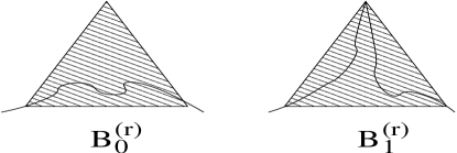
Figure 13: Restricted partition functions for the self-attracting walk for the $3$-simplex.

To calculate $G(x,u)$ for the $3$-simplex lattice, we define restricted partition functions $B_{0}^{(r)}$ and $B_{1}^{(r)}$, for walks that cross the $r$-th order triangle, as shown in Fig. 13. $B_{0}^{(r)}$ is the sum of weight of all walks that enter an $r$-th order triangle of the $3$-simplex from one corner and leave from another corner, but do not visit the third corner. $B_{1}^{(r)}$ is the sum of weights of walks that enter and leave the $r$-order triangle, and also visit the third corner of the triangle. Then it is easy to see that these weights satisfy the recursion equations

$$B_{0}^{(r+1)}=[B_{0}+B_{1}]^{2}+B_{0}[B_{0}^{2}+2B_{0}B_{1}+B_{1}^{2}u],$$ (80)

$$B_{1}^{(r+1)}=B_{1}[B_{0}^{2}+2B_{0}B_{1}+B_{1}^{2}u].$$ (81)

The generating function for all loops is given by the formula

$$P(x,u)=\sum_{r=1}^{\infty}[B_{0}^{(r)}+B_{1}^{(r)}]^{3}3^{-r}.$$ (82)

We start with the initial weights

$$B_{0}^{(1)}=0;~{}~{}B_{1}^{(1)}=x.$$ (83)

These variables tend to the trivial fixed point $B_{0}^{*}=B_{1}^{*}=0$, if the starting value of $x$ is less than a critical value $x_{c}(u)$, and to the fixed point $B_{0}^{*}=B_{1}^{*}=\infty$, if $x>x_{c}(u)$. For $x=x_{c}(u)$, $B_{1}^{(r)}$ tends to zero for large $r$, and the Eq. (80) reduces to Eq.(8). The critical properties of the chain are continuous functions of $u$, and there is no phase transition as a function of $u$.

We note that here the recursion equations involve the interaction parameter $u$. This complicates the analysis. Consider a modified problem where the interaction $-U$ occurs only between the nearest neighbor bonds in the same $2$-nd order triangle, and not otherwise. One would expect the qualitative behavior of the system very similar, but now, the recursion equations do not involve $u$. In fact, they are the same as the case without self-attraction [Eq.(8)]. This observation is helpful in studying the collapse on other fractals.

6.2 Collapse transition on $n>3$ -simplex lattices

The collapse transition on the $4$-simplex lattice was first studied in [35]. We restrict the attractive interaction to nearest neighbors within the same 2nd order simplex. Then, the recursion equations Eq. (32-33) describe the collapse transition also, if we use the starting weights

$$A^{(2)}=x^{2}+2x^{3}u+2x^{4}u^{3},\qquad{\rm and}\qquad B^{(2)}=x^{4}u^{4}.$$ (84)

Figure 14: Different fixed points for the $4$-simplex lattice. The non-trivial fixed points labelled $C$,$T$ and $S$ correspond to the collapsed, the tricritical $\theta$-point, and the swollen state.

The renormalization group flows of the variables $A$ and $B$ in this case is shown in Fig. 14. There is the trivial fixed point $A^{*}=B^{*}=0$, which is reached if $x<x_{c}(u)$. If $x>x_{c}(u)$, the fixed point $A^{*}=B^{*}=\infty$ is reached. The two-dimensional space of possible initial conditions $(A^{(1)},B^{(1)})$ is divided into the basins of attraction of these two fixed points. The common boundary of these basins is a line. This line is an invariant sub-manifold of the renormalization flows (i.e. points starting on the line remain on the line). On this line we have three fixed points :

1. The fixed point $(0.4264,.04998)$ corresponds to the swollen state. This is reached for $u<u_{c}\simeq 3.106074$ and $x=x_{c}(u)$. This is denoted by S in Fig. 14. If we start at a point near this fixed point on the critical line, the renormalization flows are towards this fixed point.

2. The fixed point $(A^{*},B^{*})=(0,22^{-1/3})$ is reached when $u>u_{c}$. It gives one relevant eigenvalues $\lambda=4$ corresponding to $\nu_{c}=1/D_{4}=1/2$. In this phase, the polymer fills the available space with a finite density of monomers. This fixed point is denoted by C in Fig. 14. This is also attractive for points starting nearby on the critical line.

3. The fixed point $(1/3,1/3)$, denoted by T in Fig. 14, is obtained for $u=u_{c}$. On the critical line $x=x_{c}(u)$, this unstable fixed point lies between the fixed points corresponding to the swollen and the collapsed phases. The matrix corresponding to linearized renormalization transformation at this point has two eigenvalues greater than one; $\lambda_{1}=3.7037$ and $\lambda_{2}=2.2222$. The third relevant eigenvalue corresponds to the renormalization of fugacity of end points ( $\lambda_{+}$ in Eq. (18)). Thus this is a tricritical point. at this point, $\nu_{c}=\ln 2/\ln\lambda_{1}=0.5239$. The singular part of the free energy varies as $(u-u_{c})^{2-\alpha}$ with

   $$\alpha=2-\frac{\ln\lambda_{1}}{\ln\lambda_{2}}=0.36027.$$ (85)

One can similarly study the $n=5$ simplex lattice [24], with the interactions are confined to the internal bonds of the second order graph. It is found that just like the $n=3$ case, there is no collapsed phase. One can understand this by noting that the ground state configuration corresponds to a walk that visits all the $5$ sites of the $2$nd order subgraph. There are many configurations corresponding to the minimum energy, and most of these are extended. Even when there is attractive interaction between all pairs of neighbors, the energy-cost of pulling a polymer confined to an $r$-th order subgraph to something that is spread over a subgraph of order $(r+1)$ is finite. As there is a large entropy associated with the place where this break occurs, this makes the collapsed phase unstable to such breaks, and brings the collapse transition temperature to zero.

In a similar way, we can study the $6$-simplex. Here we have coupled polynomial recursion equations of degree $6$ for the three variables $A^{(r)},B^{(r)}$ and $C^{(r)}$. For the details of the recursion equations, see [24]. Again, we have two trivial attractive fixed points corresponding to $(A^{*},B^{*},C^{*})$ equal to $(0,0,0)$ or $(\infty,\infty,\infty)$. There is a two-dimensional critical manifold that marks the boundary of the basins of attraction of these fixed points. For the renormalization flows on this two-dimensional critical surface, there are two attractive fixed points:

The fixed point $(A^{*},B^{*},C^{*})=(0.262352,0.017586,0.000701)$ corresponds to the swollen state as discussed in Sec. 4.1.

The fixed point $(A^{*},B^{*},C^{*})=(0,0,0.071329)$ is reached for all $u>u_{c}(=3.4999847)$ at $x=x_{c}$. The largest eigenvalue for this case is $\lambda=6$ corresponding $\nu_{c}=1/{D_{6}}=0.3869$. This describes the collapsed phase of the polymers.

The common boundary of basins of attraction of these two fixed points is a $1$- dimensional line, which is also an invariant submanifold for the renormalization flows. This line has one attractive fixed point:

The fixed point (0.12949,0.09572,0.05344) is obtained for $u=u_{c}$ and $x=x_{c}$ and has two eigenvalues greater than one; $\lambda_{1}=5.4492\;{\rm and}\;\lambda_{2}=1.9049$. This is a tricritical point with exponent $\nu_{t}=0.4088$ and $\alpha=2-\ln\lambda_{1}/\lambda_{2}=0.6309$.

The crossover exponent $\phi$ at the tricritical point is $\phi=\nu_{t}/\nu_{th}=0.3801$, where the exponent $\nu_{th}$ controls the divergence of thermal correlation and is defined as $\nu_{th}=\ln 2/\ln\lambda_{2}=1.0755$.

There are two other fixed points (0.254037, 0.022159, 0.07098) and (0.2000, 0.0666, 0.0666) on the line separating the basins of attraction of the fixed points corresponding to the collapsed and the swollen phases. These are purely repulsive, and cannot be reached starting with our choice of initial condition. These correspond to higher order multicritical points( tetra-critical).

We note that the collapse transition on fractal lattices corresponds to a new fixed point, intermediate between swollen (SAW) phase and the collapsed phase and cannot be viewed as a perturbation of the Gaussian fixed point describing random walks.

6.3 Some unusual phases

The nature of possible collapsed phases of linear polymers on fractals with a finite ramification number depends strongly on the geometrical constraints imposed by the connectivity properties of the the fractal, much more so than in the extended phase.

As we already noted, for the $n$-simplex lattice with $n$ odd, a collapsed phase with a finite density of the polymer is not found. For the modified rectangular lattice, the behavior of linear polymer with self-attraction was studied in [35]. Here the number of variables needed to describe the polymer with self-attraction becomes rather large. For example, to describe closed loops it is necessary to introduce additional weights $A_{1}^{(r)},~{}B_{1}^{(r)},A_{2}^{(r)},\ldots$ etc., where the subscript 1(2) indicates the number of extra corner sites of the $r^{th}$ -order are visited, a total of eleven variables. To describe open chains, we would need 17 additional variables, making a total of 28 variables- a rather formidable number. However, as in case of $n$-simplex lattices many of these variables are irrelevant and may be set equal to zero. Equivalently, we study collapse when the attractive interaction is restricted to the first order rectangles. If we restrict ourselves to the analysis of closed polygons, we require only the five variables defined earlier in section 4.3.

Interestingly, one finds three different phases of the polymer, depending on the value of the attraction parameter $u$. For small $u<u_{c1}=3.2023$, the polymer exists in the swollen phase, with typical size $R\sim N^{\nu}$, and $\nu=0.6650$. For large $u>u_{c2}=3.2341$, it exists in a compact phase of finite density, with $R\sim N^{1/2}$. However, between the swollen and compact phases, for $u_{c1}<u<u_{c2}$, one finds a ‘rod-like phase’, where the shape of the polymer is highly anisotropic. In the x-direction, the average extent of polymer increases as $N$, and in the other direction it remains finite. At $u=u_{c1}$, there is a non-trivial fixed point of the recursion equations of period $2$. Linear analysis of the renormalization equation about this fixed point gives $\nu=0.80503$. At $u=u_{c2}$, one gets $\nu=1/2$, same as in the collapsed phase, with possible logarithmic corrections. There is a logarithmic singularity in the specific heat also. The reason why the rod-like phase is found in this case is not clear : obviously the anisotropy of the lattice is responsible for it, but it does not matter so much in other( swollen or collapsed ) phases, where the anisotropy is of the usual type ( the ratio of average diameter of an $N$-stepped walks in the $x$- and $y$- directions is a finite number).

Another different type of phase, labelled ‘semi-compact’ phase was found by Knezevic and Vannimenus in their analysis of the collapse transition on the $HB(3,3)$ fractal [37]. In this case, the connectivity of the graph is such that a linear polymer cannot fill the available space with a finite density. For large value of the attraction strength $u$ the polymer shrinks into a “semicompact” state. In this phase, the average monomer density tends to zero for large polymers.

The recursion relations found for restricted generating functions $A^{(r)}$ and $B^{(r)}$ where $A^{(r)}$ counts the number of configurations when the polymer goes once through the $r^{th}$-order gasket while $B^{(r)}$ counts the configurations where the polymer goes twice through the gasket, are rather complicated [37], but for the large $u$ regime, the equations are dominated by only a single term in each polynomial. For large order of iteration, the recursion equations in this phase may be approximated by

$$A^{(r+1)}\simeq 320A^{3}B^{6};\qquad B^{(r+1)}\simeq 4308A^{2}B^{8}.$$ (86)

These can be linearized by taking the logarithm of both sides, which shows that for large $r$, $\log A^{(r)}$ and $\log B^{(r)}$ vary as $\lambda_{+}^{r}$, where $\lambda_{\pm}=(11\pm\sqrt{73})/2$. They will both diverge to $+\infty$, or to $-\infty$ depending upon the coefficient of proportionality being positive or negative ( both are of same sign for the largest eigenvalue). Thus, this constant must be proportional to distance from the critical line $x-x_{c}(u)$. If $x_{c}-x=\delta\ll x_{c}$, number of iterations before the deviation becomes of order 1 is

$$r_{0}\approx\log(1/\delta)/\log\lambda_{+}.$$ (87)

As the size of the polymer is approximately $2^{r_{0}}\sim(1/\delta)^{\nu^{\prime}}$, this corresponds to $\nu^{\prime}=0.48195$. The fractal dimension of the chain in this phase is, $1/\nu^{\prime}=2.07491$ a value just a bit less than the fractal dimension of the lattice $D=2.09590$. For $x=x_{c}$, $A^{(r)}$ decreases to zero as $\exp(-a\lambda_{-}^{r})$ where $a$ is some constant, and $B^{(r)}$ increases to infinity as an inverse power of $A^{(r)}$.

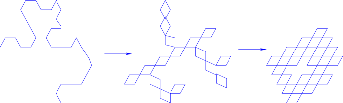
Figure 15: Schematic representation of the different phases of a linear chain with self-attraction on the Sierpinski gasket with at most two visits per site allowed: (a) the swollen phase (b) branched polymer phase with branches made of the doubled-up chain (c) the collapsed phase

In all the cases discussed so far a restriction on the walks that a lattice bond or a lattice site visited once cannot be visited again has been imposed. One can relax this condition and allow the walk to revisit a site already visited so long as no bond is traversed twice. A consistent set of visited bonds is called a trail, if different sequences in which the same set of bonds bonds may be visited are considered equivalent [38]. Orlandini et al [39] considered self-attracting SAWs on a 2d Sierpinski gasket, with this constraint, and showed that this model displays a new multicritical point corresponding to a collapse from linear into branched polymer in which the polymer becomes a randomly doubled-up chain ( see fig. 15), which is followed by a further transition into compact globule. In Fig. 15, we have drawn schematically what the different phases look like ( drawn here for the Euclidean 2-dimensional space). The universality class of the two new multicritical points corresponding to the phase transition points is different from the tricritical points discussed so far.

7 BRANCHED POLYMERS

The models of branched polymers is related to other important problems in statistical mechanics, such as lattice animals, percolation [40] and the Lee-Yang edge singularity [41]. The study of branched polymers on fractal lattices are therefore very instructive as one can analyze the system in detail. The number of different branched polymers made of $N$ monomers and their average gyration radius are expected to grow as $\mu^{N}N^{-\theta}$ and $N^{\nu}$, respectively for large $N$; $\theta$ and $\nu$ are critical exponents, whose values are different from those from that of linear polymers. If we allow loops in the cluster, we get the model of lattice animals, which corresponds to the $p\rightarrow 0$ limit of the percolation problem. These are known to be in the same universality class as branched polymers. If in addition to the excluded volume interaction, one has an attractive nearest-neighbor interaction between the monomers, the branched polymers can undergo a collapse transition, just like the linear polymers. Near the collapse point, the free energy per monomer shows singular critical behavior.

Knezevic and Vannimenus realized that real-space renormalization method for studying linear polymers on fractals can be extended directly to the case of branched polymers [42, 44]. They considered asymptotic properties of branched polymers with attractive self-interaction on fractal lattices, restricting the attractive interactions to bonds within first order units of the fractal lattices. We summarize their findings here.

7.1 The $3$-simplex lattice

The macroscopic thermodynamic quantities of interest can be obtained from the grand-partition function $G(x,u)$, whose definition is same as Eq.(79), with $\Omega(N,N_{u})$ now defined as the average number of unrooted branched polymers with $N$ bonds, and $N_{u}$ nearest neighbor bonds, the average being taken over different positions of the polymer on the fractal. This can be determined in terms of the $r$-th order restricted partition functions defined in Fig. 16.

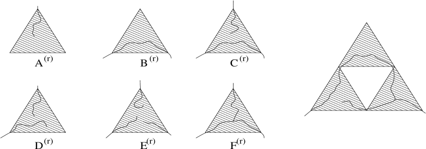
Figure 16: Diagrams representing the six restricted generating functions for branched polymers on the two dimensional Sierpinski gasket. $C^{(r)}$ corresponds, for instance, to configurations where a part of the polymer joins two vertices of an $r^{th}$ order triangle while one of its ends penetrates through the third vertex. The diagram on the right shows a term $B^{(r)}C^{(r)}F^{(r)}$ contributes to $B^{(r+1)}$.

The closed set of recursion equations involve six restricted generating functions as described in Fig 16 are easily written down [42]:

$$A^{(r+1)} = A[1+2B+2B^{2}]+2B^{2}C+F[B^{2}+A^{2}+2BD],$$

$$B^{(r+1)} = B^{2}+B^{3}+F[4BC+2AB]+F^{2}[B+D],$$ (88)

and similar equations for other variables. $G(x,u)$ can be seen as a sum of terms of the same general form as Eq. (5) and (6). The singular behavior of the sum can be analyzed by looking at the fixed points of the recursion equations. There are two trivial fixed points with all variables zero or infinite. For any given value of $u$, we have to tune the initial value of $x$ to a critical value $x_{c}(u)$ to get a non-trivial fixed point.

The analysis of the recursion equations lead to following three different nontrivial fixed points:

1. For all $u<u_{c}=5.5$, and $x=x_{c}(u)$, the recursion equations lead to a non-trivial fixed point $(A^{*},B^{*},\ldots)$ corresponding to the swollen state with large scale properties same as for the random-animal problem ($u$=1). All the fixed point values $A^{*},B^{*},\ldots$ at this fixed point are non-zero. Linear analysis of the recursion equations about this fixed point shows that the generating function $G(x,u)$ has a power-law singularity when $x=x_{c}(u)$ and the critical exponents are $\nu=0.71655$ and $\theta=0.5328$.

2. For $u>u_{c}$, and $x=x_{c}(u)$, the polymer is in the collapsed phase. The corresponding fixed point has $A^{*}=B^{*}=D^{*}=0$. $F^{(r)}$ tends to zero, and $C^{(r)}F^{(r)}$ and $E^{(r)}{F^{(r)}}^{2}$ tend to a finite limiting value. The largest value of the linearized renormalization transformation matrix is $3$, corresponding to $\nu_{c}=1/D_{3}=0.63093$. This dense phase of branched polymers is in the same universality class as the spanning trees. For the spanning trees, one can also define a chemical distance exponent $z$, by the relation $\ell\sim R^{z}$, where $\ell$ is the distance along bonds between two randomly picked points on the polymer, and $R$ is the euclidean distance. This was calculated in [43], and shown that $z=\log[(20+\sqrt{205})/15]/\log 2\simeq 1.1939$.

3. The collapse transition occurs at $u=u_{c}$. At this fixed point, all the values $A^{*},B^{*},\ldots$ are non-zero. This is a tricritical fixed point, with two eigenvalues larger than one. The exponent $\nu_{t}=0.63250$ is very close to $\nu_{c}$. The exponent $\alpha$ is negative, $\alpha=-4.0269$, showing that the singularity in the specific heat at $u=u_{c}$ is very weak.

The closeness of $\nu_{t}$ to $\nu_{c}$ has also been found on square lattice where an accurate transfer - matrix study [45] of the collapse of branched polymer gives $\nu_{t}=0.509\pm 0.003$ which is very close to the compact value 1/2. This suggests that the phenomenon is not accidental and should have a more general explanation.

The problem of linear polymers is recovered if all terms containing the functions $E$ and $F$ one suppressed in Eqs.(7.1) and (7.2). The truncated equations have only one fixed point, corresponding to the swollen phase with $\nu=0.7986$ and there is no collapsed phase (see Section 3).

7.2 The 4-simplex lattice

The closed recursion equations in this case involve eleven restricted generating functions. The number of polymer configurations to consider is large, and Knezevic and Vannimenus [44] used computer enumeration to sort them out. We omit the details.

The analysis found three non-trivial fixed points that describe the large-scale behavior of self-interacting branched polymers.

1. For $u<u_{c}\approx 2$ the random - animal fixed point corresponding to the swollen phase of the polymer is reached. Linearizing around the fixed point one finds only one relevant eigenvalues $\lambda_{1}=3.14069$. With this eigenvalue one finds $\nu=\log 2/\log\lambda_{1}=0.60566,\;{\rm and}\;\theta=0.75667$.

2. For $u>u_{c}$ one gets a fixed point corresponding to the collapsed state in which polymer occupies all vertices of the lattice. The relevant eigenvalue found in this case is $\lambda=4$ which gives $\nu_{c}=1/2$.

3. For $u=u_{c}$ the fixed point reached represents a tricritical point as it has two eigenvalues greater than $1$: $\lambda_{1}=3.94050$ and $\lambda_{2}=1.32094$. The exponent $\nu_{t}=\log 2/\log\lambda_{1}=0.50546$. This value is very close to the value $\nu_{c}=1/2$ of the collapsed phase. The exponent $\alpha=-2.8267$ is negative but less negative than for the 3-simplex lattice.

7.3 Other fractals

Knezevic and Vannimenus also studied the branched polymer problem on the $GM_{3}$ fractal [42, 44]. In this case, they found the unexpected result that unlike the case on the $GM_{2}$ fractal ( for which the behavior is the same as on the $n=3$ simplex), for the $b=3$ case, the number of animals of size $n$ grows as $\mu^{n}\exp(\kappa n^{\psi})$, where $0<\psi<1$. This corresponds to an essential singularity in the generating function of branched polymers $G(x,u=1)\sim\exp(\frac{a}{|x_{c}-x|^{\rho}})$, with $\rho=\psi/(1-\psi)$.

The analysis of Knezevic and Vannimenus has recently been extended to all $b$, and one finds that for $b\geq 3$, the average number of animals per site behaves as $\mu(b)^{n}\exp(\kappa n^{\psi})$, where the values of the the singularity exponent $\psi$, and the size exponent $\nu$ can be determined exactly [46].

8 SURFACE ADSORPTION

It is well known that a long flexible polymer in a good solvent can form a self-similar adsorbed layer near an attractive wall at the critical temperature $T_{a}$. Using the correspondence between an adsorbed polymer chain and the model of ferromagnets with $n$-vector spins in the limit $n\rightarrow 0$ with a free surface, it has been shown that the adsorption point $T_{a}$ corresponds to a tricritical point and in its proximity a crossover regime is observed. In particular, the mean number of monomers, $M$, at the surface is shown to behave as [47]

$$M = (T_{a}-T)^{(1/\phi-1)},~{}~{}~{}~{}~{}~{}~{}~{}{\rm~{}for~{}}T<T_{a};$$ (89)

$$= N^{\phi},~{}~{}~{}~{}~{}~{}~{}~{}~{}~{}{\rm~{}for~{}}T=T_{a};$$

$$= (T-T_{a})^{-1},~{}~{}~{}~{}~{}~{}~{}~{}~{}{\rm~{}for~{}}T>T_{a}.$$

A good model for this phenomenon is a SAW on some lattice with an absorbing surface (boundary). Every site on surface visited by the polymer contributes an energy $-E_{s}$. This model has widely been studied on various lattices and via a number of techniques that include exact enumeration [48, 49], Monte Carlo [50], transfer matrix [51], renormalization group [52] etc. For a 2-d Euclidean lattice, exact value of $\phi$ found from conformal field theory is 1/2 [53].

Bouchaud and Vannimenus [54] were the first to apply RSRG techniques on fractals to study the linear polymers near an attractive substrate. They showed that the known phenomenology of the adsorption -desorption transition is well-reproduced on fractals, and different critical exponents can be evaluated exactly. The values of the exponent $\phi$ for $HB(2,2)$ and $HB(2,3)$ fractals were found to be 0.5915 and 0.7481 respectively. They also showed that for a container of fractal dimension $D$ and adsorbing surface $d_{s}$, $\phi$ has lower and upper bounds;

$$1-(D-d_{s})\nu\leq\phi\leq\frac{d_{s}}{D}.$$ (90)

8.1 Surface adsorption in polymers with self-attraction

Polymer chains with self attraction near an attractive surface can exhibit a rich variety of phases, characterized by many different universality domain of critical behavior [57]. This is due to competition between the two interactions. At the intersection of two tricritical surfaces, one corresponding to the $\theta-$transition and another to the adsorption-desorption transion, one can expect higher order critical points. Understanding of the different phases that are possible and understanding and classifying the multicritical points that can exist appear difficult on standard Euclidean lattices[47]. It is here fractal lattices have been particularly helpful [58]. The values of critical exponents found are, of course, different for different fractals, but the general features of the phase-diagrams remain the same. Investigating the problem on fractals helps us understanding the problem in real experimental systems.

We consider a linear polymer chain on a truncated $n$-simplex lattice and make one boundary surface of it attractive. We treat one of the edges of the fractal container as an attractive surface and associate an energy $-E_{s}<0$ with each site on it occupied by the polymer, and an energy $E_{t}>0$, with each occupied site that is at a distance $1$ from the occupied surface i.e. on the layer adjacent to the surface, and an energy $-E_{u}$ for nearest-neighbor bond between monomers not consecutive along the chain.

Then, to each $N$-step walk having $N_{s}$ steps along the surface, $N_{t}$ steps lying on the layer adjacent to the surface and $N_{u}$ number of nearest neighbors a weight $x^{N}\omega^{N_{s}}t^{N_{t}}u^{N_{u}}$ is assigned, where $\omega=\exp(\beta E_{s})$, and $t=\exp(-\beta E_{t})$. The grand partition function for this system is given by

$$G(x,\omega,t,u)=\sum_{N,N_{s},N_{t},N_{u}}\Omega(N,N_{s},N_{t},N_{u})x^{N}\omega^{N_{s}}t^{N_{t}}u^{N_{u}},$$ (91)

where $\Omega(N,N_{s},N_{t},N_{u})$ is the number of different configurations per site of a $SAW$ of $N$ steps, rooted at a specified site on the attractive surface, with given values of $N_{s},N_{t}$ and $N_{u}$. We may put $E_{t}=0$ (or $t=1$) for simplicity, but a non-zero value seems to give rise to interesting behavior, and is also important to many physically realizable cases. The attractive interaction between monomers is restricted, as in preceding sections, to bonds within the lowest order subgraphs of the fractal lattices.

As shown in section 6.2, polymers in the n-simplex container show a collapsed phase only for even values of n. Thus, the 4- and 5-simplex lattices exhibit contrasting behavior and represent two different scenario which may arise in real systems. In the case of 5-simplex lattice, there is no collapse transition possible in the bulk, but its 4-simplex surface can show a collapsed phase. In the case of 4-simplex lattice, on the other hand, there is a collapsed globule phase in the bulk but no collapse possible in the surface-adsorbed polymer. We can therefore have situations in which the bulk acts as a poor-solvent medium, while the surface acts as a good solvent medium or the opposite case of surface being poor-solvent medium and the bulk good solvent. However, the situation in which both bulk and surface show collapsed phases can not be modelled by polymers on an $n$-simplex fractal.

8.2 The $4$-simplex lattice

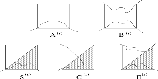
Figure 17: The restricted partition functions for the $r$th order $4$-simplex with attractive interactions at one boundary surface. The internal structure of the $4$-simplex is not shown. The shaded triangle reprsents the attractive surface.

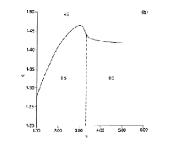
Figure 18: Sections of the $\omega-u-t$ phase diagram for two different values of $t$ for the 4-simplex lattice: (a) t= 0.2 (b) t= 0.5. Regions marked by AS, DS and DC represent, respectively, the adsorbed polymer in swollen state, desorbed polymer in swollen and collapsed (globular) state. The collapse transition between the DC and DS phases is denoted by the dashed line. The special adsorption line is indicated by full line and part of it by dotted line. The point where $\theta$-line meets with the adsorption line is a multicritical point. The dotted part of the adsorption line indicates the region of coexistence of adsorbed SAW and the (bulk) globule phase.

For the 4-simplex lattice the grand partition function of Eq. (91) can be written in terms of the five restricted partition functions shown in Fig 17. The shaded regions in the figure represent the surface. Out of five configurations, two ($A^{(r)}$ and $B^{(r)}$) represent the sum of weights of configurations of the polymer chain within one r-th order subgraph away from the surface, and the remaining three ($S^{(r)},C^{(r)}$ , and $E^{(r)}$) represent the surface functions. The recursion relations for these restricted partition functions can easily be written (see [58] for details). The equations for $A^{(r+1)}$ and $B^{(r+1)}$ do not get affected by the presence of the surface interactions.

In this case, we have three phases possible: the desorbed swollen(DS), the desorbed collapsed (DC) and the adsorbed swollen (AS) phases. The fixed points corresponding to the desorbed phases have $S^{*}=C^{*}=E^{*}=0$, and $A^{*},B^{*}$ equal to the value for the $4$-simplex at the S or C fixed point ( section 6.2). The fixed points corresponding to the polymer adsorbed on the surface, on the other hand, have $A^{*}=B^{*}=C^{*}=E^{*}=0$ and $S^{*}$ equal to the value $\mu^{-1}$ corresponding to the swollen phase fixed point on the $3$-simplex surface ( section 3.1). The phase boundaries, determined numerically by finding the basins of attraction of these fixed points are shown in Fig. 18.

If we start at any point on the boundary between the DS and AS phases, under renormalization, we flow to the symmetrical fixed point $S^{*}=C^{*}=A^{*},B^{*}=E^{*}$, with $A^{*},B^{*}$ having the value corresponding to the point $S$ in Fig. 14. Linearizing the recursion equations near this fixed point two eigenvalues $\lambda=2.7965$ (corresponding to the swollen bulk state) and $\lambda_{\phi}=2.1583$ greater than one [58] are found. This point is the expected symmetrical special absorption point which describes the polymer at the desorption transition. A simple calculation gives the crossover exponent $\phi=0.7481$ and $\alpha=0.6653$. In Fig 18, the full line shows intersection of this surface with the surface $t=$ constant.

The bulk transition between DC and DS phases is described by the fixed point $S^{*}=C^{*}=E^{*}=0$, and $A^{*}$ and $B^{*}$ have the value (1/3,1/3) corresponding to the point T in Fig. 14. This boundary has the equation $u=u_{c}$, and the value $u_{c}$ does not depend on $\omega$ or $t$.

The points on the boundary between the DC and the AS phases are found to fall in the basin of attraction of two different fixed points: $FP_{1}$ = $(A^{*}=S^{*}=C^{*}=0,B^{*}=E^{*}=0.3568)$ and $FP_{2}$= $(A^{*}=C^{*}=E^{*}=0,B^{*}=0.3568,S^{*}=0.61803)$. Correspondingly, we see two different behaviors of various quantities as we cross the AS to DC phase boundary.

The first fixed point $FP_{1}$ is reached for all points on the AS-DC surface with $t$ greater than a critical value $t^{*}$, and for large enough $u$ even for $t<t^{*}$. This has two relevant eigenvalues $\lambda_{1}=4$, and $\lambda_{2}=3$.

The fixed point $FP_{2}$ corresponds to a coexistence between the adsorbed $SAW$ and the free collapsed globule phase. In Fig 18(a), the line corresponding to this fixed point is shown by dotted line. This point is reached if $t<t^{*}$, and $u$ is greater than, but near $u_{c}$.

The line where the three phases meet is also an invariant manifold for the renormalization group flows. We find three fixed points on this line:

1. For $t<t^{*}$(= 0.34115…) the fixed point $(A^{*},B^{*},S^{*},C^{*},E^{*})$ $=$ ($\frac{1}{3}$, $\frac{1}{3}$, $0.4477$, $0.4528$, $0.0815$) is reached. The linearized equations have three repulsive directions with eigenvalues $\lambda_{SM}=2.2715,\lambda_{1}=3.7037$ and $\lambda_{2}=2.2222$. The values $\lambda_{1}$ and $\lambda_{2}$ are the same as found for the bulk $\theta$ point (see section 6.2).

2. For $t>t^{*}$ the fixed point ($\frac{1}{3},\frac{1}{3},0,0,0.3693$) is found. Again we find three eigenvalues greater than one, where $\lambda_{SM}=3$ and the other two $\lambda_{1}$ and $\lambda_{2}$ are the same as those given above.

3. For $t=t^{*}$ we find the symmetric ”disordered and collapsed” fixed point ($\frac{1}{3},\frac{1}{3},\frac{1}{3},\frac{1}{3},\frac{1}{3}$). This fixed point has four eigenvalues greater than one. These values are $\lambda_{SM_{1}}=2.7620$ and $\lambda_{SM_{2}}=1.4964...$ and the other two are $\lambda_{1}$ and $\lambda_{2}$ as given above.

The first two of these are tetracritical points, and the third point is an even higher order multicritical point ( pentacritical).

We now discuss the behavior of phase boundaries. When $t<t^{*}=0.34115$, the critical line $\omega=\omega_{c}(u,t)$ which is the phase boundary between the DS and AS phases, is almost linear with positive slope. Beyond the multicritical point, slope of the line separating the AS and the DC phases rises rather sharply. In a region specified by $u_{c}<u<u_{c_{1}}$ (the value of $u_{c_{1}}$ depends on $t$) we have the coexistence between the adsorbed SAW and the collapsed globule phase. This region is shown in Fig 18 by a dotted line. For $u>u_{c_{1}}(t)$ the line $\omega=\omega^{*}(u,t)$ becomes almost flat. The value of $u_{c_{1}}(t)$ decreases as $t$ is increased and becomes equal to that of $u_{c}$ at $t=t^{*}=0.34115$. At $t=t^{*}$ the multicritical point becomes a symmetric “desorbed and collapsed” pentacritical point having four eigenvalues greater than one.

For $t>t^{*}$ the critical line $\omega=\omega^{*}(u,t)$ has a different shape than for $t<t^{*}$. The line appears to have a maximum at $u\leq u_{c}$. It drops rather sharply (see Fig. 18(b) for t=0.5) in contrast to the case of $t<t^{*}$ at the multicritical point. Furthermore, the line $\omega=\omega^{*}(u,t)$ for $u>u_{c}$ separating the bulk collapsed and adsorbed phases shows the decreasing tendency as $u$ is increased. The two tetracritical lines on the three-dimensional $u-\omega-t$ phase space meet at a pentacritical point [58]. Along one of these tetracritical lines, the adsorbed (swollen) polymer coexists with both the desorbed polymer and the desorbed globule, and the other line is the common boundary of three critical surfaces of a continuous transition.

The behavior of the special adsorption line $\omega=\omega^{*}(u,t)$ described above can be understood from contribution of different coexisting polymer configurations to the bulk and surface free energies. When both the adsorbed and desorbed phases are in swollen state, the adsorption line has same nature in the $\omega-u$ plane for all values of $t$, although the slope of the line decreases as $t$ is increased. At $t=1$, the adsorption takes place at $\omega=1$ and the adsorption line in the $\omega-u$ plane has a zero slope. This is due to the fact that at $t=1$ and $\omega=1$ the surface is just a part of the bulk lattice. As $t$ is increased, $\omega$ has to be increased to have adsorption, and since $u$ in such a situation favors the bulk phase we have to increase the surface attraction to counteract this tendency. In the other extreme, i.e. when $u>>u_{c}$, the adsorption line has a zero slope. Here the coexisting polymer configurations are those given by $B$ and $E$ in Fig. 17. The free energies due to these two configurations balance each other at all $u$ values and therefore the line remains insensitive to the value of $u$. It is only in the neighborhood of the special $\theta$-point that the line becomes sensitive to the value of $t$ and $u$.

When $t<t^{*}$, the surface layer is strongly repulsive and prohibits the occurrence of the $E$ configurations in the neighborhood of the $\theta$-point. The adsorbed state is still given by the configuration $S$, although the bulk is in the globular compact phase. Thus to balance the free energy $\omega$ has to be increased. However, at $t>t^{*}$ the surface is only moderately repulsive and therefore at certain value of $\omega$ the polymer configuration given by $E$ is formed. Thus a lower value of $\omega$ is needed to balance the bulk free energy at the special $\theta$-point.

A casual look at Fig. 18(b) may give the impression of the existence of a re-entrant adsorbed phase as $u$ is increased. One should, however, realize that these figures are merely a projection on the $\omega$-$u$ plane of three dimensional figures in which the third dimension is given by $t$. The value of crossover exponent $\phi$ for the 4-simplex lattice is 0.7481 equal to the value found for $HB(2,3)$.

8.3 The 5-simplex lattice

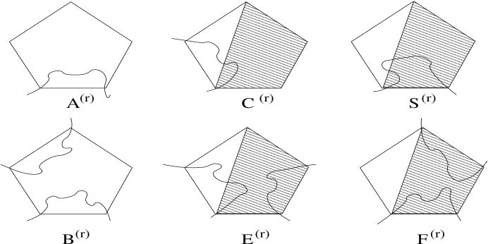
Figure 19: Restricted partition functions for the $r$th order $5$-simplex. Here $A^{(r)}$ and $B^{(r)}$ represent the bulk generating functions for the polymer chain and $S^{(r)}$, $C^{(r)}$, $E^{(r)}$ and $F^{(r)}$ represent the surface functions.

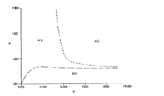
Figure 20: A section of the $\omega-u-t$ phase diagram for the $5$-simplex at a typical value of $t=0.5$. For other values of $t$, the phase boundaries shift, but the qualitative behavior is the same.

The grand partition function of Eq. (91) for 5- simplex lattice is written in terms of six restricted partition functions shown in Fig 19. Out of six configurations two ($A^{(r)}$ and $B^{(r)}$) represent the sums of weights of configurations of the polymer chain within one r-th order subgraph away from surface, and the remaining four ($C^{(r)}$, $S^{(r)}$, $E^{(r)}$ and $F^{(r)}$) represent the surface functions. As in the case of the $4$-simplex, the recursion relations for $A^{(r)}$ and $B^{(r)}$ do not include other variables.

In this case, we have three phases: The adsorbed swollen (AS), the adsorbed collapsed (AC), and the desorbed swollen (DS). It is straight forward to write down the fixed points corresponding to these phases from the known fixed points for SAWs on the $4$- and $5$- simplexs. The basins of attraction of these fixed points are shown in Fig. 20.

For the DS phase, we have $A^{*},B^{*}$ taking the value for the swollen phase of the $5$-simplex ( section 6.2), with $C^{*},S^{*},E^{*}$ and $F^{*}$ zero. In the AS and AC phases, we have $A^{*},B^{*},C^{*}$ and $E^{*}$ zero, and $S^{*},F^{*}$ has the value of corresponding the fixed points S and C respectively in Fig. 14 ($A^{*}$, $B^{*}$ in the terminology of section 6.2).

The critical surface separating the DS and AS phases is a two-dimensional surface in the $3$-dimensional parameter space $(\omega,u,t)$. All points on this surface, under renormalization, flow to the “symmetrical” fixed point $(S^{*}=C^{*}=A^{*},E^{*}=F^{*}=B^{*})$, with values of $A^{*},B^{*}$ same as for the DS fixed point. The linearization of recursion relations about this fixed point gives two eigenvalues $\lambda_{1}=3.1319$ and $\lambda_{2}=2.5858$ greater than one. The line $\omega_{c}(u,t)$ is therefore a tricritical line. The crossover exponent $\phi=0.8321$.

The AS and AC phases are separated by the critical $\theta$-surface $\omega=\omega_{c}(u,t)$ (see Fig 20). For $\omega\gg{\omega_{c}}$(u, t), this surface tends to the surface $u=u_{c}=3.316074$ in agreement with the critical value of $u$ for the collapse transition in the bulk of the 4-simplex lattice. However, in this case, this $\theta$-surface never meets the AS-DS phase boundary. It is shown in [58] that at $\omega\geq\omega_{c}(u,t)$ the $\theta$-line bends and approaches very slowly the special adsorption line $\omega_{c}(u,t)$ as the value of $u$ is increased. Even for $u=200$ the two lines have not merged. The whole AS-AC boudary corresponds to the basin of attraction of a single fixed point, and the parameter $t$ has no qualitative effect on the phase diagram.

8.4 Surface adsorption of a SAW in dimensions $2-\epsilon$

We consider the family of $GM_{b}$ fractals and evaluate the value of the exponent $\phi$ and examine its behavior as $b$ is varied from 2 to $\infty$. The energies $E_{s}$ and $E_{t}$ are defined as before. We put $E_{u}=0$ for simplicity.

A walk is called a surface walk (and assigned configuration $S$) when it enters through one corner of the surface and leaves from the other. A bulk walk represented by $B$ has no step on the surface or on the bonds connecting the surface with the bulk. A walk which enters through one corner of the surface and ends up in the bulk is assigned configuration $C$. The generating functions for these walks can be written as

$$B^{(r)}(x) = \sum B^{(r)}x^{N},$$

$$S^{(r)}(x,\omega,t) = \sum S^{(r)}(N,M,R)x^{N}\omega^{M}t^{R},$$

$$C^{(r)}(x,\omega,t) = \sum C^{(r)}(N,M,R)x^{N}\omega^{M}t^{R}.$$ (92)

Here $x$, as before, is the fugacity associated with each visited site of the lattice, $B^{(r)}(x)$ is the number of distinct configurations of the SAW which joins two vertices of the $r$th order of the fractal in the bulk and $N$ is the number of sites visited by SAW, $M$ and $R$ represent respectively, the number of visited sites of the lattice which lie on the surface and on a layer adjacent to the surface. Summations in Eqs.(85) are on the repeated indices and $S^{(r)}(N,M,R)$ and $C^{(r)}(N,M,R)$ represent number of configurations of respective walks of the r-th order gasket. The definition of parameters $\omega$ and $t$ is same as in sec. 8.1.

For $b=2$ the following three non-trivial fixed points are found:

1. The fixed point $(B^{*}=0.61803,S^{*}=C^{*}=0)$ corresponds to the bulk state with $\nu=0.7986$. For $x=x_{c}(\omega)$ the fixed point is reached for all $\omega<\omega_{c}(t)$. Note that $\omega_{c}(t)$ is a function of $t$; for $t=0.5$ the value of $\omega_{c}(0.5)$=1.1118.

2. The fixed point $(B^{*}=C^{*}=0,S^{*}=1)$ is reached for all $\omega>\omega_{c}(t)$ and $x<x_{c}(\omega)$. This represents the adsorbed state for the polymer chain with $\nu=1$, as expected for a SAW adsorbed on a line.

3. The fixed point $(B^{*}=S^{*}=C^{*}=0.61803)$ is obtained for $\omega=\omega_{c}(t)$. The linearization of Eqs.(85) about this fixed point yields two eigenvalues greater than one, i.e. $\lambda_{s}=1.6709$ and $\lambda_{b}=2.3819$. We identify this as a tricritical point. The equality of $B^{*}$, $S^{*}$ here shows that at this point the attraction at the surface, and repulsion at the next layer exactly compensate each other. The crossover exponent $\phi=\frac{\log\lambda_{s}}{\log\lambda_{b}}=0.5915$ At the point of adsorption transition the leading singular behavior of free-energy density is given as $f(T)\sim(T_{c}-T)^{2-\alpha}$ Thus the ”specific heat” exponent $\alpha$ at the tricritical point is related to $\phi$ as $\alpha=2-\frac{1}{\phi}$ for $b=2$ the value of $\alpha=0.3094$.

It is straightforward to extend this method to other members of this family. However, as the value of $b$ increases the number of possible configurations of different walks increase rapidly. For $2\leq b\leq 9$ [53,54], the value of $\phi$ found are 0.5915, 0.5573, 0.5305, 0.5089, 0.4908, 0.4753, 0.4617 and 0.4497. The value of $\phi$ decreases as $b$ increases and becomes lower than the Euclidean value of $1/2$ at $b=6$. Zivic et al [55] have used Monte Carlo renormalization-group (MCRG) method to obtain the value of $\phi$ for $2\leq b\leq 100$ and found that lower bound of Eq(84) is violated for $b=12$.

The limit $b\to\infty$ was analyzed by Kumar et al [53] using the finite size scaling theory (see sec. 5) and it was found that in this limit

$$\phi(b)=1+\nu(b)(1-D_{b})\left[1-\frac{(2\nu(b)-1)}{2}\frac{\log\log b}{\log b}+\;{\rm terms\;of\;order}\;\frac{1}{\log b}\right].$$ (93)

As for $b\to\infty$ $\nu(b)=\frac{3}{4}$, we get $\phi(\infty)=\frac{1}{4}$. The first correction to $\phi$ term to finite $b$ is proportional to $2-{\tilde{d}}_{b}$, similar to that found for $\gamma(b)$ in Eq(71). Since $\frac{2\nu(b)-1}{2}$ is positive for $\nu=\frac{3}{4}$, the first correction term in Eq(86) is negative which, when multiplied by $(1-D_{b})\nu(b)$ makes a positive contribution to $\phi(b)$. This implies that $\phi(b)$ approaches to $\frac{1}{4}$ value monotonically as $b$ is increased.

Similar to the behavior of exponent $\gamma$ for SAWs discussed in section 5, we find $\phi(b)$ does not converge to the Euclidean value in the limit $b\to\infty$. It has, however, been noted in [53] that the adsorbing surface of a fractal container is similar to that of a penetrable surface of a regular lattice in which case $\phi=1-\nu$ should be satisfied [56, 57].

9 INTERACTING WALKS

So far we were concerned with a single linear flexible polymer chain and studied its conformational properties in different environments. We now show how the critical behavior of two interacting long flexible linear polymer chains can also be studied using a lattice model of two interacting walks.

Depending on the solvent quality and the attractive interactions between intrachain and interchain monomers a system of two interacting long flexible polymer chains can acquire different configurations. The chain may be in a state of interpenetration in which the chains intermingle in such a way that they cannot be distinguished from each other. Or, the two chains may get zipped together in such a way that they lie side by side as in a double stranded DNA. It may also be possible, particularly at high temperatures, that the two chains get separated from each other without any overlap.

By varying the temperature or tuning the interaction the system can be transformed from one state to another. The point at which the zipped-unzipped transition takes place is a tricritical point and in its proximity a crossover is observed. In the asymptotic limit the mean number of monomers $M$ in contact with each other at the tricritical point is assumed to behave as

$$M\propto N^{y},$$ (94)

where $N$ is the total number of monomers in a chain and $y$ is the contact exponent.

A lattice model of two interacting walks on the $n$-simplex lattices has been developed in [61, 62, 63]. Two different situations were considered: In one, the two walks have no mutual exclusion, and a lattice bond can be occupied by one step of each walks. This model has been referred to as a model of two interacting crossed walks (TICWs). In the second model, there is mutual exclusion between chains and a lattice bond can at most be occupied by a step of either walks. This model is called a model of two interacting walks (TIWs). In a general model of two interacting walks one can associate an energy $E_{b}$ for each bond occupied by a step of both walks. The model of TICWs corresponds to $E_{b}=0$ and that of TIWs to $E_{b}=\infty$.

In the TIWs the two chains cannot be at the same site because of mutual exclusion, but there is lowering of energy if they occupy nearest neighbour sites. The strength of both the inter- and intra-chain monomer interactions depend on the solvent and chemical nature of the monomers. Let the two chains or walks be referred to as $P_{1}$ and $P_{2}$. The generating functions for this system can be written as

$$G(x_{1},x_{2};u_{1},u_{2},u_{3})=\sum_{\rm all\;walks}x_{1}^{N_{1}}u_{1}^{R_{1}}x_{2}^{N_{2}}u_{2}^{R_{2}}u_{3}^{R_{3}},$$ (95)

where $N_{1},x_{1},u_{1}$ and $R_{1}(N_{2},x_{2},u_{2}\;{\rm and}\;R_{2})$ refer, respectively, to the number of steps, fugacity weight attached to each step, the Boltzmann factor associated with the attractive interaction between monomers and the number of pairs of nearest neighbors in the chain $P_{1}(P_{2})$. $R_{3}$ is the number of pairs of monomers of different walks occupying the nearest neighbor lattice sites and $u_{3}$ denotes the Boltzmann factor associated with the attractive interaction between monomers of $P_{1}$ and $P_{2}$.

Since the individual chain can be either swollen, collapsed or at the tricritical ($\theta$) point the variables ($x_{1},u_{1}$) and ($x_{2},u_{2}$) can be taken to be known (see section 6.2). Therefore, Eq.(89) has only $u_{3}$ as independent variable. With these simplifications it has become possible to evaluate the restricted generating functions for the $n$-simplex lattices.

From the generating function of Eq.(89) one can calculate the average number of monomers of the two chains which are in contact (nearest neighbor) with each other from the relation

$$\langle R_{3}\rangle=u_{3}\frac{\partial\log G}{\partial u_{3}}.$$ (96)

The RSRG transformation has been used in [60, 61] for $n$-simplex lattices to solve the model exactly and calculate the phase diagram and the value of $y$ for the different conditions of the solvent.

Since the topological structure of a $3$-simplex lattice is such that it can not have two SAWs on it, the model of TIWs was solved on the $4$,$5$ and $6$ simplex lattices. These lattices can have two interacting SAWs, with possible self-attraction also, without the walks crossing each other at any lattice point. On the 3- and 4- simplex lattices TICWs model in a condition in which both chains are in the swollen state has been solved in [61].

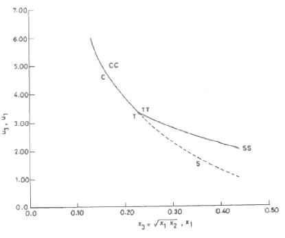
Figure 21: The state of a system of two polymer chains in a non-selective solvent on the 4-simplex lattice in the $x_{3}({=\sqrt{x_{1}x_{2}}}),u_{3}$ plane. Lines $SS$ and $CC$ represent the tricritical lines of the zipped state of two chains each in the swollen state and the interpenetration state of the chains in a compact globule phase, respectively. Point $TT$, at which these lines meet, represents a transition point from a segregated to an interpenetrated state of the chains each at its $\theta$ point. For a given value of $x_{3}$ which corresponds to the swollen state of both chains, the chains are in interpenetrated state when the value of $u_{3}$ is less than the value given by the line $SS$. For the value of $x_{3}$ corresponding to the chains in their compact globule state or at their $\theta$ points, the two chains are in the segregated state for all values of $u_{3}$ less than the value given by the line $CC$ or point $TT$. We also show the $x-u$ phase diagram of a single chain for comparison’s sake. Note that the line $CC$ overlaps with line $C,TT$ with point $T$.

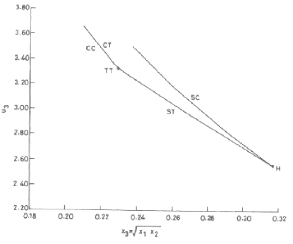
Figure 22: The phase diagram of a system of two chains in a selective solvent on the 4-simplex lattice in the $x_{3}(={\sqrt{x_{1}x_{2}}}),u_{3}$ plane. Lines $SC$ and $ST$ respectively, represent the interpenetration states of two chains when one chain is in a swollen state and other is in compact globule phase or at its $\theta$ point. Line $CT$ corresponds to the configuration of interpenetration of the chains when one in the compact globule phase and the other is at its $\theta-$point. When the value of $u_{3}$ is less than that given by corresponding lines, the two chains are segregated from each other.

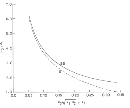
Figure 23: The phase diagram representing the configurations of a system of two chains on the 5-simplex lattice in the $x_{3}(={\sqrt{x_{1}x_{2}}}),u_{3}$ plane. Line $SS$, as in Fig 22, represents the zipped state of the chains. For all values of $u_{3}$ less than the value given by line $SS$, the two chains intermingle with each other. Line $S$ represents the swollen state of a chain.

9.1 TIW’s on the 4-simplex lattice

To describe the two walks on the 4-simplex lattice we need five restricted partition functions. Two of these, $A^{(r)}$ and $B^{(r)}$ defined in Fig 11 correspond to the walk $P_{1}$ and identical functions $C^{(r)}$ and $D^{(r)}$ correspond to walk $P_{2}$. The restricted partition function $E^{(r)}$ represents the configurations where walks $P_{1}$ and $P_{2}$ occupy neighboring sites and is sum of weights of configurations in which walks $P_{1}$ and $P_{2}$ enter and exit the r-th order subgraph once each. The two corner vertices of the subgraph are occupied by the walk $P_{1}$ and the other two corner vertices by walk $P_{2}$. The recursion relation for the generating function $E^{(r)}$ involves both $A^{(r)}$, $B^{(r)}$ and $C^{(r)}$, $D^{(r)}$ and is written as[60],

$$E^{(r+1)}=A^{2}C^{2}+2ACE(A+C)+2E^{4}+6E^{2}(B^{2}+D^{2})+4E^{3}(B+D).$$ (97)

As shown in sec. 6.2, a polymer chain on a 4-simplex lattice can be in any one of the states of the swollen, compact globule and the $\theta$-point and is described in the asymptotic limit by the fixed points (0.4294.., 0.04998..), (0, $22^{-\frac{1}{3}}$) and ($\frac{1}{3},\frac{1}{3}$), respectively. The fixed points corresponding to a swollen state is reached for all values of $u_{1}$ (or $u_{2}$) $<u_{c}$=3.31607 at $x_{1}$ (or $x_{2}$)=$x_{c}$. The value of $x_{c}$ is a function of the interaction $u_{1}$ (or $u_{2}$). The end to end distance for a chain of N-monomers in this state varies as $N^{\nu}$ with $\nu$=0.7294… . The fixed point corresponding to the compact globule state is reached for all values of $u_{1}$ (or $u_{2}$) $>u_{c}$ (i.e. at low temperatures) at $x_{1}$(or $x_{2}$)=$x_{c}(u_{i})$, where i=1 or 2. In a compact globule state the polymer chain has a finite density of the monomer per site when N$\rightarrow\infty$. At $u_{1}$(or $u_{2}$)=$u_{c}$=3.31607 and $x_{1}$(or $x_{2}$)=$x_{c}$($u_{c}$)=0.22913… the $\theta$-point state is reached.

In a system of two chemically different polymer chains, we may have six independent combinations of the individual chains which we indicate by $SS,CC,TT,SC,ST$ and $CT$, where letters $S,C$ and $T$ now stand for the swollen, compact globule and $\theta$-point states. The recursion relation (91) is solved using the fixed points ($A^{*},B^{*}$) and ($C^{*},D^{*}$) corresponding to the given states of the chain $P_{1}$ and $P_{2}$ and the starting weight $E^{(1)}=(x_{1}x_{2})^{2}u_{3}^{4}$. The solution leads to two fixed points denoted as $E_{s}^{*}$ and $E_{i}^{*}$ for each combination of states of the individual chains. In table I the values of these fixed points, relevant eigenvalues and the contact exponents $y$ at the tricritical points are listed [62]. Figs. 19 and 20 show the state of two chains in the $x_{3}(={\sqrt{x_{1}x_{2}}}),u_{3}$ plane respectively, for non-selective and selective solvents.

Lines $SS$ and $CC$ in Fig. 19 represent the tricritical lines of the zipped states of two chains each in the swollen state and the interpenetrating state of the chains each in a compact globule phase, respectively. Point $TT$, at which these lines meet, represents a transition point from a segregated to an interpenetrated state of the chains each at its $\theta$ point. For a given value of $x_{3}$ which corresponds to a swollen state of both chains, the chains are in the interpenetrated state when the value of $u_{3}$ is less than the value given by the line $SS$. For the values of $x_{3}$, corresponding to the chains in their compact globule state or at their $\theta$-point, the two chains are in a segregated state for all values of $u_{3}$ less than the values given by line $CC$ or point $TT$. The $x,u$ phase diagram of a single chain is also given in the figure for the comparison sake.

The state of two interacting chains in a selective solvent on the $4$-simplex lattice is shown in Fig 20. Lines $SC$ and $ST$, respectively, represent the interpenetration state of two chains when one is in the compact globule phase or at its $\theta$-point. Line $CT$ corresponds to the configuration of the interpenetration of the chains when one is in the compact globule phase and the other is at its $\theta$-point. When the value of $u_{3}$ is less than given by the corresponding lines, the two chains are segregated from each other. The individual chains configuration remains unchanged whether they are segregated or intermingled.

9.2 TIW’s on the 5-simplex lattice

For the 5-simplex lattice we also need five restricted partition functions to describe the generating functions of two walks; two corresponding to walk $P_{1}$, two corresponding to walk $P_{2}$ and $E^{(r)}$ which represents the configurations in which walks $P_{1}$ and $P_{2}$ enter and exit the r-th order subgraph once each and may occupy neighboring sites. The recursion relation for $E^{(r)}$ in this case is lengthy[60] and is therefore not reproduced here.

As already shown in section 6.2 a polymer chain always remains in a swollen state for all values of interaction, (self-) attraction on a 5-simplex lattice. This state is characterized by the fixed point (0.3265…, 0.0279…). In this case we therefore have only one combination, i.e. $SS$ of chains. Using these values of fixed points for single chains, the recursion relation for the partition function $E^{(r)}$ of two interacting chains (see [62]) is solved and fixed points $E_{s}^{*}=0.0279$ or $E_{i}^{*}=0.2713$ are found. The fixed point $E_{s}^{*}$ is found for all values of $u_{3}<u_{3c}(x_{3})$. At $u_{3}=u_{3c}(x_{3})$ fixed point $E_{i}^{*}$ is found.

Table 1: Values of fixed points, relevant eigenvalues, and the contact exponent $y$ at the critical point for the 4-simplex lattice. The swollen, compact globule, and the tricritical configuration of each chain is indicated by letters $S,C,\;{\rm and}\;T$ respectively. $\lambda_{1}$ is the largest eigenvalue of the system, and $\lambda_{i}$ refers to the two chain configuration point.

State
of individual chains	$E^{*}_{s}$	$E^{*}_{i}$	$\lambda_{i}$	$\lambda_{1}$	$y$
SS	0.04998	0.6125	2.6420	2.7965	0.9447
CC	0.0	22-1/3	2.5440	4.0	0.6735
TT	0.01484	1/3	2.2222	3.7037	0.6098
SC	0.0	0.4880	2.8520	4.0	0.7559
ST	0.02687	0.4294	2.8526	3.7037	0.6311
TC	0.0	0.3680	2.5740	4.0	0.6820

Table 2: Values of fixed points, $G_{s}^{*},H_{s}^{*},I_{s}^{*},G_{I}^{*},H_{I}^{*}$ and $I_{I}^{*}$. The labeling is the same as in Table 1, but for 6-simplex.

State	$G^{*}_{s}$	$H^{*}_{s}$	$I^{*}_{s}$	$G^{*}_{i}$	$H^{*}_{i}$	$I^{*}_{i}$	$\lambda_{i}$	$\lambda_{1}$	$y$
of ind.
chains
SS	0.0175	0.0007	0.0007	0.1406	0.0147	0.0147	2.2054	3.4965	0.6318
CC	0.0	0.0	0.0	0.0	0.0713	0.0713	4.2201	0.6318	0.7902
TT	5.4$\times 10^{-4}$	5.4$\times 10^{-4}$	5.4$\times 10^{-4}$	0.0957	0.0535	0.0535	3.2225	5.4492	0.6902
SC	0.0	0.0	0.0	6.75$\times 10^{-5}$	0.1049	0.0711	5.0529	6.0	0.9041
ST	0.0028	0.0003	0.001	0.229	0.1047	0.0776	5.2434	5.4492	0.9659
CT	0.0	0.0	0.0	0.0060	0.0714	0.0806	4.4019	6.0	0.8271

In Fig. 21, $u_{3}$ is plotted as a function of $x_{3}=\sqrt{x_{1c}x_{2c}}$. The interpenetrated state is found for all values of $u_{3}$ which lie below lines $SS$ at a given $x_{3}$. When the values of $u_{3}$ reaches a value given by the line $SS$, the two chains are zipped together. Line $S$ indicates the critical values of fugacity $x_{c}$ and the self-attraction $u_{1}$ (or $u_{2}$) of a polymer chain.

9.3 TIW’s on the 6-simplex lattice

In this case one needs nine generating functions[60]; three corresponding to chain $P_{1}$, three corresponding to chain $P_{2}$ and the remaining three denoted as $G^{(r)}$, $H^{(r)}$, and $I^{(r)}$ represent, respectively, the sum of weights of configurations in which walks $P_{1}$ and $P_{2}$ enter and exit the r-th order subgraph once each, $P_{1}$ twice and $P_{2}$ once, and $P_{1}$ once and $P_{2}$ twice. Since the 6-simplex lattice exhibits the collapse transition there are six independent combinations of single chain states, similar to the case of 4-simplex lattice. The fixed points corresponding to single chains found in section 6.2 have been used to find the fixed points of the recursion relation for the restricted partition functions for $G,H,$ and $I$ with suitable starting weights [62]. The values of fixed points , corresponding eigenvalues and contact exponents are given in table II. The qualitative features of the phase diagram found for this lattice are the same as that of the 4-simplex lattice.

Though the model of TIW’s discussed above ignores the effects of one chain on the critical behavior of the other chains, it provides a qualitative description of the phase diagram of systems of two polymer chains in a solution which may have different qualities for different chains and may serve as a starting point for more thorough investigation of segregation and entanglements in a real systems. The phase diagrams plotted here are in the plane $x_{3}(={\sqrt{x_{1}x_{2}}}$, $u_{3}$. Plot of phase diagrams in a three-dimensional $u_{1},u_{2},u_{3}$ space is expected to give more informations about the states the two interacting chains.

10 CONCLUDING REMARKS

It seems fair to say that the study of linear and branched polymers on fractals has been very useful in developing a better understanding of the critical behavior of polymers. One can verify the general qualitative features of the polymers on fractals which are very often similar to that in real experimental systems. One has a good deal of freedom in selecting the details of the fractal, and this can be used to find one that represents best the local geometry of the space. The exact values of the critical exponents do depend on the details of the fractal. But what is more important is that one can handle the different interactions in the problem, between different monomers, with the substrate, or with a different chain consistently and satisfactorily in way that allows exact calculation.

Of course there are many unsolved problems, and possible directions for further research in this area. The most interesting problem would be to try to extend these exact solutions to some fractals with infinite ramification index. There are some studies of statistical physics models of interacting degrees of freedom on Sierpinski carpets, using Monte Carlo simulations, or approximate renormalization group using bond-moving, or other ad-hoc approximations. An exactly soluble case would be very instructive here.

Determination of the exact scaling functions, not just the critical exponents, for these problems would be instructive: For example, the exact functional form of the scaling function of the probability distribution of the end-to-end distance of the SAW’s on these fractal, or the periodic function of Fig. 8. For a numerical study of the former, see [64]. Solving the SAW problem with quenched disorder is another interesting question. For the $3$-simplex fractal, this corresponds to making the variables $B^{(r)}$ random variables, and one has to determine the probability distribution of this variable for large $r$.

We have discussed only the equilibrium properties of polymers. Of course, in many real systems, the time scales for equilibriation can be very large. It is thus of interest to study non-equilibrium properties of statistical mechanical systems on fractals. A simple prototype is the study of kinetic Ising model on fractals. Closer to our interests here, one can study, say, the reptation motion of a polymer on the fractal substrate. This seems to be a rather good first model of motion of a polymer in gels.

It is a pleasure to thank Sumedha for a careful reading of the manuscript, and her many constructive suggestions for an improved presentation.

References

- [1] M.E. Fisher and M. F. Sykes, Phys. Rev., 114 (1959) 45.
- [2] P. G. de Gennes, Scaling Concepts in Polymer Physics, (Cornell University Press, Ithaca, London, 1979).
- [3] N. Madras and G. Slade, The Self-Avoiding Walk, (Birkhauser, Boston,1993); D. S. McKenzie, Phys. Rep. C 27 (1976) 35; Polymer Physics: 25 Years of the Edwards Model, Ed. S. M. Bhattacharjee, (World Scientific, Singapore, 1992); K. Y. Lin and Y. C. Hsaio, Chinese J. Phys. 31 (1993) 695; A. J. Guttmann, in Computer Aided Statistical Physics, Ed. C. K. Hu, A.I.P. Conf. Proc. Vol. 248, (1992) 34.
- [4] B. Nienhuis, Phys. Rev. Lett. 49 (1982) 1062.
- [5] I. Jensen and A. J. Guttmann, J. Phys. A: Math. Gen. 32 (1999) 4867.
- [6] B. Duplantier and H. Saleur, Nucl. Phys. B 290 (FS 20) (1987) 291.
- [7] T. Hara and G. Slade, Comm. Math. Phys. 147 (1992) 101; ibid Rev. Math. Phys. 4(1992) 235.
- [8] K. Wilson and J. Kogut, Phys. Rep. C 12 (1974) 75.
- [9] F. E. Stillinger, J. Math. Phys. 18 (1977) 1244.
- [10] D. Dhar, in Polymer Physics: 25 years of the Edwards’ Model, Ed. S. M. Bhattacharjee, ( World Scientific, Singapore, 1992), 83.
- [11] D. R. Nelson and M. E. Fisher, Ann. Phys.(NY) 91 (1975) 226.
- [12] D. Dhar, J. Math. Phys. 18 (1977) 577.
- [13] J. A. Given and B. B. Mandelbrot, J. Phys. A 16 (1983) L565.
- [14] D. Dhar, J. Phys. A 21 (1988) 2261.
- [15] R. Hilfer and A. Blumen, J. Phys. A: Math. Gen. 17 (1984) L537.
- [16] S. Milosevic, D. Stassinupoulos and H. E. Stanley, J. Phys. A 21 (1988) 1477.
- [17] D. Dhar, J. Math. Phys. 19 ( 1978) 5.
- [18] R. Rammal G. Toulouse and J. Vannimenus, J. Phys. (Paris) 45 (1984) 389.
- [19] T. Hattori and T. Tsuda, J. Stat. Phys. 109 (2002) 39.
- [20] D. Sornette, Phys. Rep. 297 (1998) 239.
- [21] S. Milosevic, I Zivic, and S. Elezovic Hadzic, Phys. Rev. E 61 (2000) 2141.
- [22] Sumedha and D. Dhar, (2004), in preparation.
- [23] S. Kumar, Y. Singh and Y. P. Joshi, J. Phys. A: Math. Gen. 23 (1990) 2987.
- [24] S. Kumar and Y. Singh, J. Phys. A: Math. Gen. 23 (1990) 5115
- [25] J. R. Melrose, J. Phys. A : Math. and Gen. 18 (1985), L17; and references cited therein.
- [26] S. Elezovic, M. Knezevic and S. Milosevic, J. Phys. A 20 (1987) 1215.
- [27] V. Bubanja and M. Knezevic, cited in [30].
- [28] D. Dhar, J. Phys. (Paris), 49 ( 1988) 397.
- [29] J. Cardy and S. Redner, J. Phys A: Math and Gen. A 17 (1984) L933.
- [30] S. Milosevic and I Zivic, J. Phys A 24 (1991) L833.
- [31] I. Zivic and S. Milosevic, J. Phys. A 26 (1993) 3393.
- [32] A. J. Guttmann and G. M. Torrie, J. Phys. A: Math and Gen 17 (1984) 3541.
- [33] K. Tanaka, Sci. Am. 244(1) (1981) 110; J. des Cloiseaux and G. Jannink; Polymers in Solutions (Clarendon, Oxford 1990).
- [34] D. J. Klein and W. A. Seitz, J. Physique Lett. 45 (1984) L241.
- [35] D. Dhar and J. Vannimenus, J. Phys. A: Math. Gen.20, (1987) 199.
- [36] S. Kumar and Y. Singh, Phys. Rev. A 42 (1990) 7151.
- [37] M. Knezevic and J. Vannimenus, J. Phys. A: Math.Gen. 20 (1987) L969.
- [38] A. Malakis, J. Phys. A: Math. Gen. 9 (1976) 1283.
- [39] E. Orlandini, F. Seno, A. L. Stella and M. C. Tesi Phys. Rev. Lett. 68 (1992) 488.
- [40] A. B. Harris and T. C. Lubensky, Phys. Rev. B 24(1981) 2656; T. C. Lubensky and J. Isaacson, Phys. Rev. Lett. 41(1978) 829, Phys. Rev.A 20 (1979) 2130.
- [41] G. Parisi and N. Sourlas, Phys. Rev. Lett. 46 (1981) 871; D. C. Bridges and J. Z. Imbrie, Ann. Math. 158 (2003) 1019.
- [42] M. Knezevic and J. Vannimenus, Phys. Rev. Lett. 56 (1986) 1591.
- [43] D. Dhar and A. Dhar, Phys. Rev. E 55 (1997) R 2093.
- [44] M. Knezevic and J. Vannimenus, Phys. Rev. B 35 (1987) 4988.
- [45] B. Derrida and H. Herrmann, J. Phys.(Paris) 44 (1983) 1365.
- [46] D. Dhar, (2004), submitted for publication.
- [47] K. De’Bell and T. Lookman, Rev. Mod. Phys. 65 (1993) 87.
- [48] R. Rajesh, D. Dhar, D. Giri, S. Kumar and Y. Singh, Phys. Rev. E 65 (2002) 056124.
- [49] Y. Singh, S. Kumar and D. Giri, J. Phys. A: Math. Gen 32, L407, (1999); 34 (2001) L67.
- [50] P. Grassberger and R. Hegger, Phys. Rev. E 51 (1995) 2674.
- [51] A. R. Veal, J.M. Yeomans and G. J. Jug, J. Phys. A: Math. Gen 24 (1991) 827.
- [52] S. Kumar and Y. Singh, Physica A 229 (1996) 61.
- [53] T. W. Burkhardt, E. Eisenriegler and I. Guim, Nucl. Phys. B 316 (1989) 559.
- [54] E. Bouchaud and J. Vannimenus, J. Physique 50 (1989) 2931.
- [55] S. Kumar, Y. Singh and D. Dhar, J. Phys. A:Math. Gen. 26 (1993) 4835.
- [56] V. Bubanja, M. Knezevic and J. Vannimenus, J. Stat. Phys. 71 (1993) 1.
- [57] I. Zivic, S. Milosevic and H.E. Stanley, Phys. Rev. E 49 (1994) 636.
- [58] T. Ischinabe, J. Chem. Phys. 80 (1984) 1318.
- [59] Y. Singh, S. Kumar and D. Giri, Pramana J. of Phys. 53 (1999) 37.
- [60] S. Kumar and Y. Singh, Phys. Rev. E 48 (1993) 734.
- [61] S. Kumar and Y. Singh, J. Phys. A:Math and Gen. 26 (1993) L987.
- [62] S. Kumar and Y. Singh, Phys. Rev. E 51 (1995) 579.
- [63] S. Kumar and Y. Singh, J. Stat. Phys. 89 (1997) 981.
- [64] A. Ordemann, M. Porto, and H. E. Roman, Phys. Rev. E 65 (2002) 021107.