Folding of the triangular lattice in a discrete three-dimensional space: Crumpling transitions in the negative-bending-rigidity regime

Abstract

Folding of the triangular lattice in a discrete three-dimensional space is studied numerically. Such “discrete folding” was introduced by Bowick and co-workers as a simplified version of the polymerized membrane in thermal equilibrium. According to their cluster-variation method (CVM) analysis, there appear various types of phases as the bending rigidity $K$ changes in the range $-\infty<K<\infty$. In this paper, we investigate the $K<0$ regime, for which the CVM analysis with the single-hexagon-cluster approximation predicts two types of (crumpling) transitions of both continuous and discontinuous characters. We diagonalized the transfer matrix for the strip widths up to $L=26$ with the aid of the density-matrix renormalization group. Thereby, we found that discontinuous transitions occur successively at $K=-0.76(1)$ and $-0.32(1)$. Actually, these transitions are accompanied with distinct hysteresis effects. On the contrary, the latent-heat releases are suppressed considerably as $Q=0.03(2)$ and $0.04(2)$ for respective transitions. These results indicate that the singularity of crumpling transition can turn into a weak-first-order type by appreciating the fluctuations beyond a meanfield level.

I Introduction

A model of “discrete folding” was introduced as a possible lattice realization (discretized version) for the tethered (polymerized) membranes in thermal equilibrium Kantor90 ; DiFrancesco94a ; DiFrancesco94b ; Cirillo96b ; Bowick95 ; Cirillo96 ; Bowick96 ; Bowick97 . The constituent molecules of the tethered membranes are connected with each other via polymerization Nelson89 ; Nelson96 ; Bowick01 . Hence, the in-plane strain is subjected to finite shear moduli. In this sense, the tethered membranes are stiff, compared with the fluid membranes Canham70 ; Helfrich73 for which the constituent molecules are diffusive, and cannot support a shear. Reflecting this peculiarity, the tethered membranes get flattened macroscopically at sufficiently low temperatures (or equivalently large bending rigidities) Nelson87 . This phase transition is called the crumpling transition. (Because the crumpling transition occurs even in the absence of the self-avoidance, we neglect this effect throughout this paper.) The flat phase is characterized by the long-range orientational order of the surface normals. It would be remarkable that such an $O(3)$ symmetry, namely, an orientational order, breaks spontaneously for a two-dimensional manifold. Actually, it has been known that the fluid membranes are always crumpled irrespective of the temperatures. To clarify the nature of the crumpling transition of the tethered membranes, a good deal of theoretical analyses have been reported so far. However, there still remain controversies whether the singularity belongs to a continuous phase transition Kantor86 ; Kantor87 ; Baig89 ; Ambjorn89 ; Renken96 ; Harnish96 ; Baig94 ; Bowick96b ; Wheater93 ; Wheater96 ; David88 ; Doussal92 ; Espriu96 or a discontinuous one accompanied with appreciable latent-heat release Paczuski88 ; Kownacki02 . Actually, in numerical simulations, it is not quite obvious to rule out a possibility of weak-first-order phase transition Kantor87b ; Kantor87c .

As would be anticipated, an approach via the discrete-folding model Bowick95 ; Cirillo96 ; Bowick96 ; Bowick97 is promising to resolve this longstanding issue: In fact, the discrete-folding model reduces to a mere Ising magnet Bowick95 with a dual transformation; we explain the details afterward. The Ising variables, however, are subjected to a constraint, which makes the thermodynamics rather nontrivial. Nevertheless, once formulating the discrete folding in terms of the Ising variable, we are able to resort to a variety of techniques developed in the study of magnetism: Cirillo and co-workers carried out an extensive cluster-variation method (CVM) analysis with the single-hexagon-cluster approximation Cirillo96 ; Bowick97 . Remarkably enough, according to their CVM solution, various types of phases emerge as the bending rigidity $K$ changes; see Fig. 1 for a schematic drawing of the phase diagram. As depicted in the figure, the symbols, $K_{P3}$, $K_{G3}$, and $K_{C3}$, specify the respective crumpling-transition points separating the piled-up, tetrahedral, octahedral, and totally-flat phases; we followed the notation in Ref. Bowick97 .

Stimulated by their result, in an earlier paper Nishiyama04 , we performed a first-principles simulation for the discrete folding. Our simulation scheme is based on the transfer-matrix diagonalization with the aid of the density-matrix renormalization group White92 ; White93 ; Nishino95 ; Nishiyama02 ; Nishiyama03 . In Ref. Nishiyama04 , we dwelt on the $K>0$ regime, and investigated the crumpling transition at $K=K_{C3}$: We estimated the transition point as $K_{C3}=0.195(2)$, and estimated the amount of the latent heat as $Q=0.365(5)$. Moreover, we confirmed that for $K>K_{C3}$, the entropy disappears completely as predicted by the CVM analysis Cirillo96 . That is, the membrane stretches out into a totally flat sheet in that regime. In this sense, the transition at $K=K_{C3}$ is rather peculiar, and it would be less relevant to that of the realistic tethered membranes. Beside slight quantitative discrepancies concerning the folding entropy at $K=0$ and the amount of the latent heat, our simulation data support the CVM predictions, implying that the membrane undulations beyond a single-hexagon cluster are not quite significant in the $K>0$ regime.

In this paper, we devote ourselves to the $K<0$ regime, where the CVM analysis predicts two types of crumpling transitions Bowick97 . Our aim is to examine the singularities of these transitions with the density-matrix renormalization group for $L\leq 26$: It is conceivable that the order of the transition changes or that even the transition disappears by appreciating the fluctuations beyond the single-hexagon-cluster level. As a consequence, we found that the crumpling transitions occur at $K=-0.76(1)$ and $-0.32(1)$, and the singularities are both discontinuous. Actually, we estimated the amounts of the latent heat as $Q=0.03(2)$ and $0.04(2)$, respectively. Our result indicates that the singularity of the crumpling transition can change into a (weak) first-order type by fully appreciating the fluctuations.

In fairness, it has to be mentioned that the discrete folding has been studied extensively with computer simulations other than the density-matrix renormalization group, namely, the conventional full-diagonalization scheme Bowick96 ; Bowick97 and the Monte Carlo method Pujol04 : In the full-diagonalization calculation, the tractable systems sizes are limited within $L\leq 6$, and are not feasible for identifying the characters of the transitions. In fact, as for the transition at $K=K_{P3}$, it was speculated that no sign of the transition could be captured until $L=8$, which is far beyond the ability of the full-diagonalization scheme. On the other hand, the Monte Carlo simulation suffers from a very slow relaxation to the thermal equilibrium (glassy behavior). Although such a metastability is a fascinating topic in its own right, it brings about a severe obstacle to an efficient sampling in thermal equilibrium. (Such slow relaxation is to be attributed to the constraint to the Ising variables.) We stress that the density-matrix renormalization group is capable of treating large system sizes, and free from the slow-relaxation problem.

The rest of this paper is organized as follows. In the following section, we give an account of the discrete folding, following the presentation in Ref. Bowick95 . Then, we explain the density-matrix renormalization group adopted to the discrete-folding model Nishiyama04 . In Sec. III, we present the numerical results. The last section is devoted to the summary and discussions.

II Diagonalization of the transfer matrix with the density-matrix renormalization group: A brief reminder of Ref. Nishiyama04

In this section, we explain an outline of our simulation scheme. Full account of details will be found in an earlier paper Nishiyama04 . To begin with, we introduce the discrete folding of the triangular lattice in a discretized three-dimensional space Bowick95 .

II.1 Discrete folding in three dimensions Bowick95

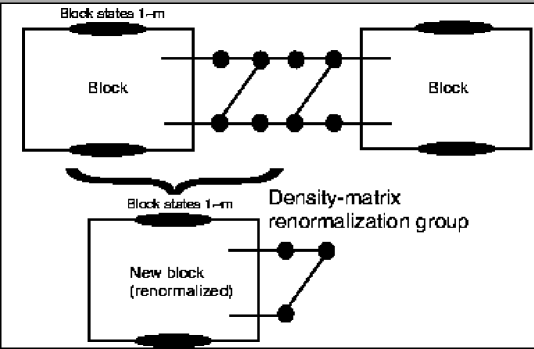
Figure 3: Schematic drawing of the density-matrix renormalization group (DMRG) procedure. From the drawing, we see that through one operation of DMRG, a “block” and the adjacent sites (hexagon) are renormalized altogether into a new renormalized “block.” At this time, the number of block states is retained within $m$; see text for details. In this manner, we can diagonalize a large-scale transfer matrix through sequential applications of DMRG.

Let us explain how the triangular lattice is folded (embedded) in a discrete three-dimensional space, namely, the face-centered cubic (fcc) lattice. As shown in Fig. 3 of Ref. Bowick95 , the fcc lattice is viewed as a close packing of two types of polygons, namely, the octahedrons and tetrahedrons, whose vertexes are shearing the fcc-lattice points; the faces of these polygons are all equilateral triangles. Hence, wrapping these polygons with a sheet of the triangular lattice, we are able to embed the sheet arbitrarily in the fcc lattice. More specifically, the relative fold angles $\theta$ between adjacent triangles are taken from four possibilities, namely, “no fold” ($\theta=\pi$), “complete fold” ($\theta=0$) “acute fold” ($\theta=acos(1/3)$), and “obtuse fold” ($\theta=acos(-1/3)$).

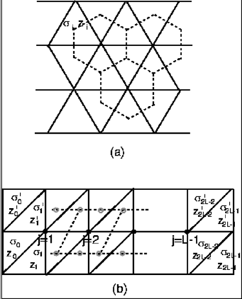
Figure 2: (a) We consider a discrete folding of the triangular lattice embedded in the three-dimensional space. In order to specify the fold angle, we place two types of Ising variables such as $z_{i}$ and $\sigma_{i}$ at each triangle rather than at each joint (gauge rule Bowick95 ). Hence, hereafter, we consider a spin model defined on the dual (hexagonal) lattice. (b) A construction of the transfer matrix. The row-to-row statistical weight yields the transfer-matrix element. The explicit formula is given by Eq. (1). The transfer matrix is diagonalized with the density-matrix renormalization group; see Fig. 3.

The above discretization leads to an Ising-spin representation for the discrete folding. An efficient representation, the so-called gauge rule, reads as follows Bowick95 : We place two types of Ising variables, namely, $\sigma_{i}$ and $z_{i}$, at each triangle (rather than each joint); see Fig. 2 (a). The gauge rule states that these Ising spins specify the joint angle between the adjacent triangles. That is, provided that the $z$ spins are antiparallel ($z_{1}z_{2}=-1$) for a pair of adjacent neighbors, the joint angle is either acute or obtuse fold. Similarly, if $\sigma_{1}\sigma_{2}=-1$ holds, the relative angle is either complete or obtuse fold. Note that the above rules specify the joint angle unambiguously. To summarize, we introduced Ising variables placed at each triangle. Because the structure dual to the triangular lattice is hexagonal, the Ising variables constitute an Ising model on the hexagon lattice. Hence, the transfer-matrix strip looks like that drawn in Fig. 2 (b). The row-to-row statistical weight $T_{\{\sigma_{i},z_{i}\},\{\sigma_{i}^{\prime},z_{i}^{\prime}\}}$ yields the transfer-matrix element. However, according to Ref. Bowick95 , the Ising variables are not quite independent, but subjected to some constraints for each hexagon. The transfer-matrix element is given by the following form with extra factors that enforce the constraints Bowick95 ;

$$T_{\{z,\sigma\},\{z^{\prime},\sigma^{\prime}\}}=(\prod_{j=1}^{L-1}U_{j}V_{j})\exp(-H/T),$$ (1)

with,

$$U_{j}=\delta(\sigma_{2j-2}+\sigma_{2j-1}+\sigma_{2j}+\sigma^{\prime}_{2j-1}+\sigma^{\prime}_{2j}+\sigma^{\prime}_{2j+1}\ mod\ 3,0),$$ (2)

and,

$$V_{j}=\prod_{c=1}^{2}\delta(\alpha_{c}(z_{2j},z_{2j-1},z_{2j-2},z^{\prime}_{2j-1},z^{\prime}_{2j},z^{\prime}_{2j+1})\ mod\ 2,0).$$ (3)

Here, $\delta(m,n)$ denotes Kronecker’s symbol, and $\alpha_{c}$ is given by,

$$\alpha_{c}(z_{1},\dots,z_{6})=\sum_{i=1}^{6}\frac{1}{2}(1-z_{i}z_{i+1})\delta(c_{0}+\sum_{j=1}^{i}\sigma_{i}-c\ mod\ 3,0).$$ (4)

The Boltzmann factor $\exp(-H/T)$ in Eq. (1) is due to the bending-energy cost. Hereafter, we choose the temperature $T$ as the unit of energy; namely, we set $T=1$. As usual, the bending energy is given by the inner product, $\cos\theta_{ij}$ of the surface normals of adjacent triangles. Hence, the bending energy is given by the formula;

$$H=-0.5\sum_{\langle ij\rangle}K\cos\theta_{ij}=-0.5\sum_{\langle ij\rangle}\frac{1}{3}K\sigma_{i}\sigma_{j}(1+2z_{i}z_{j}),$$ (5)

with the bending rigidity $K$. Here, the summation $\sum_{\langle ij\rangle}$ runs over all possible nearest-neighbor pairs $\langle ij\rangle$ around each hexagon. (The overall factor $0.5$ is intended to reconcile the double counting.) The above completes a prescription to construct the transfer matrix. In the following, we explain how we diagonalized the transfer matrix.

II.2 Diagonalization of the transfer matrix for the discrete folding: An application of the density-matrix renormalization group Nishiyama04

As would be apparent from Fig. 2 (b), a unit cell contains four Ising variables. Therefore, the size of the transfer matrix grows rapidly in the form $16^{L}\times 16^{L}$ with the system size $L$. Hence, the diagonalization of the transfer matrix requires huge computer-memory space. (Actually, with the conventional full-diagonalization scheme, the tractable systems sizes are limited within $L\leq 6$ Bowick95 ; Bowick96 ; Bowick97 .) In order to cope with this difficulty, in an earlier paper Nishiyama04 , we developed an alternative (memory saving) diagonalization method based on the density-matrix renormalization group. White92 ; White93 ; Nishino95 . In the following, we outline the algorithm, placing an emphasis on the changes specific to this problem; refer to a textbook Peschel99 for a pedagogical guide.

The density-matrix renormalization group is based on the idea of the (computer aided) real-space decimation. We presented a schematic drawing of one operation of the real-space-decimation procedure in Fig. 3. Through the decimation, the block states and the adjacent spin variables (hexagon) are renormalized altogether into a new block states. Note that through the decimation, the number of states for the (renormalized) block is truncated within $m$; the parameter $m$ sets the simulation precision. Hence, sequential applications of the procedure enable us to reach very long system sizes. In order to reduce the truncation error, we need to retain $m$ significant bases. According to the criterion advocated in Ref. White92 ; White93 , such $m$ states are chosen from the eigenstates of the (local) density matrix with dominant statistical weights (large eigenvalues) $\{w_{\alpha}\}$ ($\alpha$: integer index) Peschel99 .

This is a good position to address a few remarks regarding the changes specific to the present problem. First, in our simulation, in order to reduce the truncation error of the real-space decimation, we adopted the “finite-size method” White93 ; Peschel99 . Secondly, we applied a magnetic field $h$ at an end of the transfer-matrix strip. Namely, we incorporated an additional Hamiltonian of the form $-h\delta_{\sigma,1}\delta_{z,1}$ with $h=0.05$ and the edge spins $(\sigma,z)$. This trick was utilized in the preceding full-diagonalization calculation Bowick97 , and it aims to split off the degeneracy caused by the trivial four-fold symmetry ($\sigma=\pm 1,z=\pm 1$) of the overall membrane orientation (gauge redundancy).

III Numerical results

In this section, based on the algorithm explained above, we perform computer simulations for the discrete-folding model in the negative bending rigidity ($K<0$) regime. As a preliminary survey, we calculate the order parameters, Eqs. (6)-(7), for a wide range of $K$. Thereby, we examine the phase diagram predicted by the CVM analysis as depicted in Fig. 1. We will also provide a distribution of the density-matrix eigenvalues in order to elucidate the reliability of the present scheme. These preliminary analyses are followed by large-scale simulations to determine the singularities of the crumpling transitions precisely.

III.1 Preliminary survey: A check of the reliability of the simulation scheme

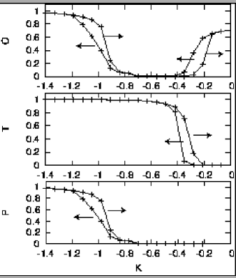
Figure 4: The order parameters, Eqs. (6)-(8), are calculated with the density-matrix renormalization group for the system size $L=14$ and the number of states kept for a block $m=12$. The arrows indicate the directions of the parameter sweeps. We notice that the behaviors are similar to those obtained with the CVM analysis (see Fig. 1). However, contrary to the prediction, the simulation data exhibit clear evidences of the hysteresis effects for both transitions, implying that these transitions are both discontinuous.

In Fig. 4, we plotted the following order parameters (local magnetizations) Bowick97 for the system size $L=14$ and the number of states remained for a renormalized block $m=12$;

$$O = \langle\sigma_{s}\rangle$$ (6)

$$T = \langle z\sigma_{s}\rangle$$ (7)

$$P = \langle z\rangle,$$ (8)

where the bracket $\langle\cdots\rangle$ denotes the thermal average, and the symbol $\sigma_{s}$ stands for the staggered component of the moment $\sigma$. (Non-zero magnetizations are induced by the symmetry-breaking field at an end; see Sec. II for details.) As depicted in Fig. 1, the CVM analysis predicts successive crumpling transitions with varying the bending rigidity $K$, and these phases are characterized by the above order parameters. Indeed, our simulation data support this claim; namely, there appear crumpling transitions at $K\approx-0.9$ and $-0.3$ successively. However, on closer inspection, our simulation data exhibit clear evidences of the hysteresis effects for both transitions. Hence, contrary to the CVM scenario, both transitions should be of discontinuous characters.

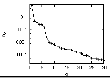
Figure 5: Distribution of the eigenvalues (statistical weights) $\{w_{\alpha}\}$ ($\alpha$, integer index) of the (local) density matrix White92 ; White93 ; Nishino95 is shown. The simulation parameters are chosen from the bending rigidity $K=-0.2$, the number of states kept for a block $m=15$, and the system size $L=15$. We see that $w_{\alpha}$ drops very rapidly for large $\alpha$. Because we discard the irrelevant states $\alpha>m$, the weight $w_{\alpha}$ at $\alpha=m$ yields an indicator of the truncation error. We attain a precision of the order $5\times 10^{-4}$ under setting $m=15$ for instance.

Before going into detailed analysis of the hysteresis effects, let us check the reliability of the scheme. In Fig. 5, we show the distribution of the statistical weights (eigenvalues of the density matrix) $\{w_{\alpha}\}$ for $K=-0.2$, $L=15$ and $m=15$. We see that the statistical weight drops very rapidly. In other words, a majority of the statistical weight concentrates on a few dominant (relevant) states.

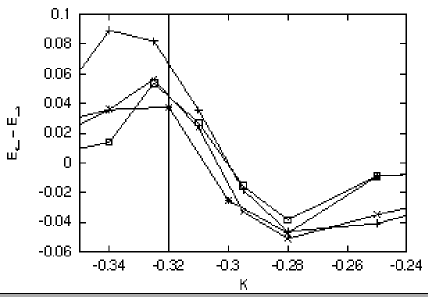
Figure 8: Residual internal energy $E_{\leftarrow}-E_{\rightarrow}$ per triangle is plotted for ($+$) $L=18$ and $m=15$, ($\times$) $L=20$ and $m=15$, ($\ast$) $L=22$ and $m=15$, and ($\Box$) $L=24$ and $m=15$. From the residual internal energy at the transition point, we estimate the latent heat as $Q=0.04(2)$.

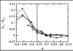
Figure 10: Residual internal energy $E_{\leftarrow}-E_{\rightarrow}$ per triangle is plotted for ($+$) $L=19$ and $m=15$, ($\times$) $L=20$ and $m=15$, ($\ast$) $L=22$ and $m=20$, and ($\Box$) $L=26$ and $m=15$. From the residual internal energy at the transition point, we estimate the latent heat as $Q=0.03(2)$.

From the data, we are able to read off a reliability of the numerical simulation: Because we discard those states with the indexes $\alpha>m$ through an operation of the renormalization-group procedure, the statistical weight $w_{\alpha}$ at $\alpha=m$ yields an indicator of the truncation error. To be specific, the fifteenth state, for instance, exhibits a very tiny statistical weight $w_{15}\approx 5\times 10^{-4}$. This truncation error accounts for a precision of the free energy. The reliability of other quantities such as the internal energy $E$ could be enhanced by a factor of 10; namely, the precision would be of the order $\sim 5\times 10^{-3}$. The data scatter of Figs. 8 and 10, for instance, should be attributed to this uncertainty. Moreover, it is to be noted that the strength of bending rigidity set in Fig. 5, namely, $|K|=0.2$, is rather small. Therefore, upon stiffening the rigidity $|K|$ further, the fluctuations get suppressed, and correspondingly, the truncation error improves. In particular, for $|K|>0.7(\approx|K_{P3}|)$, such an improvement appears to be pronounced. Encouraged by these findings, we proceed to large-scale simulations to determine the singularities of the crumpling transitions.

III.2 Singularity of the crumpling transition at $K=K_{G3}$

In the above, we observed clear evidences of the onsets of the crumpling transitions at $K\approx-0.9$ and $-0.3$. Contrary to the CVM scenario, these transitions are both discontinuous. Here, performing large-scale simulations, we confirm that the transitions are indeed discontinuous ones accompanied with appreciable latent-heat releases.

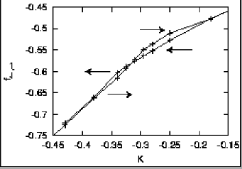
Figure 6: Free energy per triangle $f_{\rightarrow,\leftarrow}$ is plotted for $L=20$ and $m=15$. These subscripts, $\rightarrow$ and $\leftarrow$, specify the directions of the parameter sweeps, namely, the ascending and descending directions, respectively. We see that at $K\approx-0.3$, a first-order phase transition occurs.

We first consider the crumpling transition at $K=K_{G3}$, namely, the transition separating the tetrahedral and octahedral phases. In Fig. 6, we plotted the free energy per triangle $f_{\rightarrow,\leftarrow}$ for $L=20$, and $m=15$. (See our preceding paper Nishiyama04 for an algorithm to calculate the free energy reliably.) As indicated in the plot, we swept the parameter $K$ in both descending and ascending directions. Correspondingly, the indexes of $f_{\leftarrow}$ and $f_{\rightarrow}$ specify the parameter-sweep directions. From the data, we observe a clear hysteresis effect; the intersection point of $f_{\rightarrow}$ and $f_{\leftarrow}$ yields the location of the first-order phase transition. Therefore, we confirm that the crumpling transition at $K=K_{G3}$ is indeed a first-order phase transition.

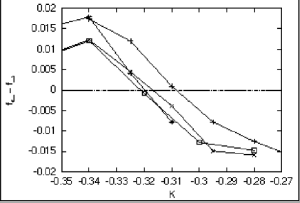
Figure 7: Excess free energy $f_{\leftarrow}-f_{\rightarrow}$ is plotted for ($+$) $L=18$ and $m=15$, ($\times$) $L=20$ and $m=15$, ($\ast$) $L=20$ and $m=20$, and ($\Box$) $L=22$ and $m=15$. From the coexistence criterion $f_{\leftarrow}-f_{\rightarrow}=0$, we determined the transition point as $K=-0.32(1)$.

In order to determine the transition point more precisely, in Fig. 7, we plotted the excess free energy $f_{\leftarrow}-f_{\rightarrow}$ for various values of $L$ and $m$. From the figure, we see that the data for $L\geq 20$ converge to the thermodynamic limit satisfactorily. From the coexistence condition $f_{\leftarrow}-f_{\rightarrow}=0$, we estimate the transition point as $K=-0.32(1)$. The location of the transition point is in good agreement with the CVM result $K=-0.294$.

In order to estimate the latent heat, in Fig. 8, we plotted the residual internal energy $E_{\leftarrow}-E_{\rightarrow}$ per triangle for various values of $L$ and $m$. Similar to the above, the data, $E_{\rightarrow}$ and $E_{\leftarrow}$, are calculated by sweeping $K$ in ascending and descending directions, respectively. The residual internal energy at the transition point $K=-0.32(1)$ yields the latent heat. The data for $L\geq 20$ appear to reach the thermodynamic limit satisfactorily. From these data, we determine the latent heat as $Q=0.04(2)$. The present estimate is not consistent with the CVM result $Q=0.14$; this value is taken from Fig. 12 of Ref. Bowick97 . We see that the discrepancy between the present estimate and the CVM analysis with a single-hexagon-cluster approximation is rather severe, and it may indicate that the fluctuations beyond a hexagon cluster are not quite negligible. Such fluctuations contribute to smearing out the latent-heat release significantly.

Although the latent-heat release acquires such a notable suppression, there appears a distinct hysteresis effect as shown in Figs. 4 and 6. This peculiarity may be reflected in the preceding full-diagonalization calculation for $L\leq 6$ Bowick97 : This calculation captures an evidence of the onset of the transition by a steep increase of the order parameter $T$, whereas the character of the singularity was remained unsolved. Actually, such a small amount of latent heat could hardly be resolved by conventional approaches. Nevertheless, such peculiarities, namely, a small latent heat and a distinct hysteresis effect, suggest that the barrier between the coexisting states is hardly surmountable, albeit these states are rather close to each other in the configuration space, To the best of our knowledge, such a feature is specific to the crumpling transition, and it may be related to the anomalous metastability (glassy behavior) observed in the Monte Carlo simulation Pujol04 .

Lastly, let us address a technical remark on the hysteresis effect. The hysteresis cannot be reproduced by the conventional full-diagonalization scheme. In the density-matrix renormalization group, on the contrary, in the course of simulation, past information is encoded (retained) in the renormalized block through the sequential applications of normalizations. Because of this “memory effect” Gendiar02 , the density-matrix renormalization group reproduces a hysteresis behavior. Beside this advantage, the method admits reliable estimate for the free energy. These advantages are significant to determine the first-order-phase-transition point reliably.

III.3 Singularity of the crumpling transition at $K=K_{P3}$

Let us turn to surveying the singularity at $K=K_{P3}$, namely, the crumpling transition separating the piled-up and tetragonal phases; note that according to CVM, the transition should be continuous.

In Fig. 9, we plotted the excess free energy $f_{\leftarrow}-f_{\rightarrow}$ for various values of $L$ and $m$. The data exhibit a clear hysteresis effect. Hence, we confirm that contrary to the CVM scenario, the transition is of a discontinuous character. From the coexistence condition $f_{\leftarrow}-f_{\rightarrow}=0$, we determine the transition point as $K=-0.76(1)$. The location of the transition point is consistent with the CVM estimate $K=-0.852$. Hence, apart from the singularity characterization, the CVM treatment appears to be justified.

The discrepancy between the present numerical result and the CVM analysis suggests that just like the above mentioned case of $K=K_{G3}$, the fluctuations beyond a hexagon cluster are important. As a matter of fact, the preceding full-diagonalization analysis for $L\leq 6$ Bowick97 could not even detect a sign of singularity around $K=K_{P3}$, and the authors speculated that the singularity would not be captured correctly until $L=8$. In other words, we need to consider long-length-scale fluctuations exceeding $L=8$, at least, in order to capture the characteristics of this transition. In this sense, the crumpling transitions in the $K<0$ regime are much more subtle than that of $K>0$ studied previously in Refs. Bowick96 ; Nishiyama04 .

Moreover, as shown in Fig. 9, the behavior of the excess free energy $f_{\leftarrow}-f_{\rightarrow}$ is asymmetric with respect to the transition point $K=-0.76(1)$; namely, the absolute value of the excess free energy is enhanced in the $K<-0.76$ side, whereas in the other size $K>-0.76$, it remains suppressed. (Note that as for $K\sim K_{G3}$, for both sides of the transition, the excess free energy behaves quite similarly (symmetrically) as shown in Fig. 7.) A large amount of the excess free energy reflects an existence of strong metastability. In fact, as shown in Fig. 4, the order parameters exhibit notable hysteresis effects in the regime $K<-0.76$. That is the reason why a symptom of the transition implied by the hysteresis curve deviates significantly from the true transition point determined by the coexistence condition (zero excess free energy) $f_{\leftarrow}-f_{\rightarrow}=0$. We suspect that the hexagon-cluster-approximation CVM estimate $K_{P3}=-0.852$, which is slightly smaller than ours $K_{P3}=-0.76(1)$, could also be biased by this asymmetry. Nevertheless, as mentioned in the Monte Carlo simulation Pujol04 , such a metastability, reminiscent of that of the spin glasses, is quite peculiar, and further details have be clarified so as to confirm the present simulation result.

In order to estimate the latent heat, we plotted the residual internal energy $E_{\leftarrow}-E_{\rightarrow}$ in Fig. 10. From the residual internal energy at the transition point, we estimate the latent heat as $Q=0.03(2)$. As noted above, such a finite latent-heat release is due to the fluctuation effect beyond a meanfield level. It is to be noted however, in the present case of $K=K_{P3}$, the fluctuation effect leads to enhancing the latent-heat release rather than smearing it out as in the above mentioned case of $K=K_{G3}$.

We notice that the amount of the latent heat is considerably suppressed. (Note that the latent heat at $K=K_{C3}(>0)$ is much larger $Q=0.365(5)$ Nishiyama04 . ) Our simulation result suggests that the long-length-scale fluctuations beyond the meanfield treatment can drive the transition to a weak-first-order type. As mentioned in Introduction, the singularity of the crumpling transition for (realistic) membranes is arousing controversies. In this respect, the present result cautions us not to rule out the possibility of weak-first-order type very easily so as to avoid misidentifying it with a continuous one of an unknown universality class. Nevertheless, we suspect that the transition in the $K<0$ side is relevant to the crumpling transition of (realistic) tethered membranes rather than the transition in the other side $K<0$, whose discontinuous character is too pronounced.

According to the analytical theory Bowick97 , the crumpling transition at $K=K_{P3}$ is equivalent to that of the two-dimensional (planar) folding Kantor90 ; DiFrancesco94a ; DiFrancesco94b ; Cirillo96b , which exhibits a continuous transition in $K<0$ Cirillo96b . Hence, provided that this equivalence holds, the crumpling transition at $K=K_{P3}$ should be continuous as well. This mapping is based on the idea that for large $|K|$, the complete and acute folds are dominant, and within this restricted configuration space, the discrete folding is equivalent to the planar folding. However, our simulation result does not support this claim, and rather, it suggests that the restricted-configuration picture would not be validated. Possibly, a slight violation of such a restriction alters the transition singularity into a weak-first-order type. In other words, in reality, various types of fluctuations are promoted around $K=K_{P3}$, and such fluctuations give rise to a finite latent-heat release.

IV Summary and discussions

We investigated the singularities of the crumpling transitions of the discrete-folding model in the negative-bending-rigidity regime $K<0$. We adopted the density-matrix renormalization group to diagonalize the transfer matrix for the strip widths up to $L=26$; the system sizes treated here are substantially larger than those tractable with the conventional full-diagonalization scheme $L\leq 6$ Bowick97 . Actually, in Ref. Bowick97 , it was speculated that the singularity at $K=K_{P3}$ would not be captured correctly until $L=8$. Hence, it is significant to consider long-length-scale undulations exceeding $L=8$. In order to check the reliability of the present simulation, we calculated the distribution of the density-matrix eigenvalues (statistical weights) for $L=15$ and $K=-0.2$. From the data, we found that the truncation error due to the renormalization group (real-space decimation) procedure is of the order $\sim 5\times 10^{-4}$ for $m=15$ (number of bases remained for a renormalized block). This result is encouraging in the sense that the truncation error is smaller than the finite-size corrections, and in practice, almost negligible.

As a preliminary survey, we calculated the order parameters, Eqs. (6)-(8), for a wide range of $K(<0)$. The overall behaviors support the CVM scenario as depicted in Fig. 1; namely, there appear two crumpling transitions around $K\approx-0.9$ and $-0.3$, which separate the piled-up, tetragonal and octahedral phases. However, on closer inspection, we observe clear hysteresis effects for both transitions. That is, contrary to the CVM scenario, both singularities should be discontinuous.

Performing large-scale simulations, we determined the transition points as $K=-0.76(1)$ and $-0.32(1)$. At respective transition points, we estimated the amounts of the latent heat as $Q=0.03(2)$ and $0.04(2)$. Comparing the present results with the CVM estimates with the single-hexagon-cluster approximation, namely, $Q=0$ ($K_{P3}=-0.852$) and $0.14$ ($K_{G3}=-0.294$), we notice that the discrepancies between them are rather conspicuous. The present simulation results suggest that the fluctuations beyond a hexagon cluster are significant. According to Ref. Bowick97 , the transition at $K=K_{P3}$ should be a continuous one, provided that complete and acute folds are dominant around the transition point; within this restricted configuration space, the discrete folding is equivalent to the planar (two-dimensional) folding, which exhibits a continuous transition in $K<0$. However, our simulation does not support this claim, because the transition turns out to be of a discontinuous character.

In an earlier paper Nishiyama04 , we studied the crumpling transition in $K>0$, and reported that it belongs to a first-order phase transition with the latent heat $Q=0.365(5)$. Consequently, it turns out that all crumpling transitions of the discrete-folding model are discontinuous. However, it is notable that the amounts of the latent heat in $K<0$ are much smaller than that of the other side $K>0$. In other words, the singularities of the crumpling transitions in $K<0$ are all weak-first-order phase transitions. As mentioned in Introduction, on the contrary, a majority of Monte Carlo simulation for (realistic) tethered membranes has reported that the crumpling transition should be a second-order phase transition Kantor86 ; Kantor87 ; Baig89 ; Ambjorn89 ; Renken96 ; Harnish96 ; Baig94 ; Bowick96b ; Wheater93 ; Wheater96 ; David88 ; Doussal92 ; Espriu96 . However, as noted in Refs. Kantor87b ; Kantor87c , it is not quite obvious to rule out the possibility of weak first-order transition in practice. Hence, it would be desirable to set forward the present analysis to other discretized-membrane models, such as the square-diagonal-lattice folding and its variants DiFrancesco98a ; DiFrancesco98b ; Cirillo00 , in order to see whether the crumpling transitions are still of discontinuous characters (weak first order); the discretized-membrane model admits detailed analysis on the character of the crumpling transition. This problem will be addressed in future study.

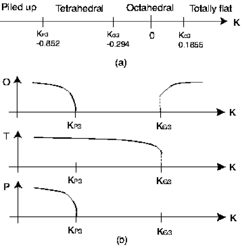
Figure 1: (a) A phase diagram of the discrete folding model determined with the cluster-variation method (CVM) Bowick97 . Various phases appear as the bending rigidity $K$ changes. (b) A schematic drawing of the behaviors of the order parameters, Eqs. (6)-(7), determined with CVM Bowick97 ; this result is to be compared with our first-principles-simulation data as shown in Fig. 4. Note that according to CVM, the transition at $K_{P3}$ ($K_{G3}$) should be a continuous (discontinuous) one.

Figure 9: Excess free energy $f_{\leftarrow}-f_{\rightarrow}$ is plotted for ($+$) $L=18$ and $m=20$, ($\times$) $L=20$ and $m=15$, ($\ast$) $L=22$ and $m=15$, and ($\Box$) $L=22$ and $m=20$. From the coexistence criterion $f_{\leftarrow}-f_{\rightarrow}=0$, we determined the transition point as $K=-0.76(1)$.

- (1) Y. Kantor and M. V. Jarić, Europhys. Lett. 11, 157 (1990).
- (2) P. Di Francesco and E. Guitter, Europhys. Lett. 26, 455 (1994).
- (3) P. Di Francesco and E. Guitter, Phys. Rev. E 50, 4418 (1994).
- (4) E. N. M. Cirillo, G. Gonnella and A. Pelizzola, Phys. Rev. E 53, 1479 (1996).
- (5) M. Bowick, P. Di Francesco, O. Golinelli and E. Guitter, Nucl. Phys. B 450, 463 (1995).
- (6) E. N. M. Cirillo, G. Gonnella and A. Pelizzola, Phys. Rev. E 53, 3253 (1996).
- (7) M. Bowick, P. Di Francesco, O. Golinelli and E. Guitter, Condensed Matter and Hight-Energy Physics (World Scientific, Singapore).
- (8) M. Bowick, O. Golinelli, E. Guitter and S. Mori, Nucl. Phys. B 495, 583 (1997).
- (9) D. Nelson, T. Piran and S. Weinberg, Statistical Mechanics of Membranes and Surfaces, Volume 5 of the Jerusalem Winter School for Theoretical Physics (World Scientific, Singapore, 1989).
- (10) P. Ginsparg, F. David and J. Zinn-Justin, Fluctuating Geometries in Statistical Mechanics and Field Theory (Elsevier Science, The Netherlands, 1996).
- (11) M. J. Bowick and A. Travesset, Phys. Rep. 344, 255 (2001).
- (12) P. Canham, J. Theor. Biol. 26, 61 (1970).
- (13) W. Helfrich, Z. Naturforsch. C 28, 693 (1973).
- (14) D. R. Nelson and L. Peliti, J. Phys. (France) 48, 1085 (1987).
- (15) Y. Kantor, M. Kardar and D. R. Nelson, Phys. Rev. Lett. 57, 791 (1986).
- (16) Y. Kantor, M. Kardar and D. R. Nelson, Phys. Rev. A 35, 3056 (1987).
- (17) M. Baig, D. Espriu and J. Wheater, Nucl. Phys. B 314, 587 (1989).
- (18) J. Ambjørn, B. Durhuus and T. Jonsson, Nucl. Phys. B 316, 526 (1989).
- (19) R. Renken and J. Kogut, Nucl. Phys. B 342, 753 (1990).
- (20) R. Harnish and J. Wheater, Nucl. Phys. B 350, 861 (1991).
- (21) M. Baig, D. Espiu and A. Travesset, Nucl. Phys. B 426, 575 (1994).
- (22) M. Bowick, S. Catterall, M. Falcioni, G. Thorleifsson and K. Anagnostopoulos, J. Phys. I (France) 6, 1321 (1996).
- (23) J. F. Wheater and P. Stephenson, Phys. Lett. B 302, 447 (1993).
- (24) J. F. Wheater, Nucl. Phys. B 458, 671 (1996).
- (25) F. David and E. Guitter, Europhys. Lett. 5, 709 (1988).
- (26) P. Le Doussal and L. Radzihovsky, Phys. Rev. Lett. 69, 1209 (1992).
- (27) D. Espriu and A. Travesset, Nucl. Phys. B 468, 514 (1996).
- (28) M. Paczuski, M. Kardar and D. R. Nelson, Phys. Rev. Lett. 60, 2638 (1988).
- (29) J.-Ph. Kownacki and H. T. Diep, Phys. Rev. E 66, 066105 (2002).
- (30) Y. Kantor and D. R. Nelson, Phys. Rev. Lett. 58, 2774 (1987).
- (31) Y. Kantor and D. R. Nelson, Phys. Rev. A 36, 4020 (1987).
- (32) Y. Nishiyama, Phys. Rev. E 70, 016101 (2004).
- (33) S. R. White, Phys. Rev. Lett. 69, 2863 (1992).
- (34) S. R. White, Phys. Rev. B 48, 10345 (1993).
- (35) T. Nishino, J. Phys. Soc. Jpn. 64, 3598 (1995).
- (36) Y. Nishiyama, Phys. Rev. E 66, 061907 (2002).
- (37) Y. Nishiyama, Phys. Rev. E 68, 031901 (2003).
- (38) C. Castelnovo, P. Pujol, and C. Chamon, Phys. Rev. B 69, 104529 (2004).
- (39) I. Peschel, X. Wang, M. Kaulke and K. Hallberg, Density-Matrix Renormalization: A New Numerical Method in Physics (Springer-Verlag, Berlin, 1999).
- (40) A. Gendiar, and T. Nishino, Phys. Rev. E 65, 046702 (2002).
- (41) P. Di Francesco, Nucl. Phys. B 525, 507 (1998).
- (42) P. Di Francesco, Nucl. Phys. B 528, 453 (1998).
- (43) E. N. M. Cirillo, G. Gonnella, and A. Pelizzola, Nucl. Phys. B 583, 584 (2000).