Fermi arcs and the hidden zeros of the Green’s function in the pseudogap state

Abstract

We investigate the low energy properties of a correlated metal in the proximity of a Mott insulator within the Hubbard model in two dimensions. We introduce a new version of the Cellular Dynamical Mean Field Theory using cumulants as the basic irreducible objects. These are used for re-constructing the lattice quantities from their cluster counterparts. The zero temperature one particle Green’s function is characterized by the appearance of lines of zeros, in addition to a Fermi surface which changes topology as a function of doping. We show that these features are intimately connected to the opening of a pseudogap in the one particle spectrum and provide a simple picture for the appearance of Fermi arcs.

The origin of the pseudogap persists as one of the leading unresolved problems in the physics of the copper-oxide high temperature superconductorsHTCS . Since a lot of the physics of these systems arise from short range correlations, cluster extensions of single site Dynamical Mean Field Theory (DMFT)review are ideally suited for this problem. In fact, using such methodologies, several groups have foundpsgap that a pseudogap, as evidenced by a suppression of the density of states at the Fermi level, appears near the doped Mott insulator as described by the Hubbard model. This effect is caused solely by short-range correlations and no long range order or preformed pairs need to be invoked. In the present work we present an extension of the cluster methodology that allows us to identifying the emergence of lines of zeros of the Green’s function at zero energy (i.e. the Luttinger surface) in addition to the quasiparticle poles (i.e. the Fermi surface), in the proximity to the Mott transition. These results are similar to those found in quasi one-dimensional systems by Essler and Tsveliktsve . The appearance and the evolution of a pseudogap in the particle spectral function is governed by the topology of these lines. At small hole doping, the Fermi surface, i.e. the line of poles, is a hole pocket having a Luttinger surface in close proximity. The quasiparticle weights along a portion of the Fermi contour are suppressed by the proximity of the zero line, generating the Fermi arc behavior of the spectral function which was identified experimentally exper .

We formulate a new cluster approach based on a re-summation of a strong coupling expansion around the atomic limit, which generalizes the CDMFT approachcdmft . We use the notations of Ref.paper1, , for a general lattice Hamiltonian,

$$H = H_{0}+H_{1}$$

$$= \sum_{i}\sum_{\alpha}\lambda_{\alpha}X_{i}^{\alpha\alpha}+\sum_{i\neq j}\sum_{\alpha,\beta,\alpha^{\prime},\beta^{\prime}}E_{ij}^{\alpha\beta\alpha^{\prime}\beta^{\prime}}X_{i}^{\alpha\beta}X_{j}^{\alpha^{\prime}\beta^{\prime}},$$

where the local, $H_{0}$, and the non-local, $H_{1}$, terms are expressed in terms of Hubbard operators, $X_{i}^{\alpha\beta}$. Here $\alpha,\beta,\alpha^{\prime}$ and $\beta^{\prime}$ represent single-site states. All the on-site contributions, like, for example, the Hubbard U interaction, are included in $\lambda_{\alpha}$, while the non-local coupling constants $E_{ij}^{\alpha\beta\alpha^{\prime}\beta^{\prime}}$ can be understood as generalized hopping matrix elements and may include hopping terms ($t_{ij}$), spin-spin interactions ($J_{ij}$), or non-local Coulomb interactions ($V_{ij}$).

A cluster DMFT schemecdmft maps the lattice model onto an effective impurity problem on a real space cluster ${\mathcal{C}}$, defined by the statistical operator

$$e^{-\beta H_{c0}}\hat{T}\exp\left\{-\int_{0}^{\beta}d\tau\int_{0}^{\beta}d\tau\prime~{}X_{a}^{\mu}(\tau)\left[\Delta_{ab}^{\mu\nu}(\tau-\tau^{\prime})\right.\right.$$

$$+\left.\left.\delta_{\tau,\tau^{\prime}}E_{ab}^{\mu\nu}\right]X_{b}^{\nu}(\tau^{\prime})+\int_{0}^{\beta}d\tau~{}h_{a}^{\mu}(\tau)X_{a}^{\mu}(\tau)\right\},$$ (2)

where $H_{c0}=\sum_{a\in\mathcal{C}}\sum_{\alpha}\lambda_{\alpha}X_{a}^{\alpha\alpha}$ is the local cluster Hamiltonian, $\hat{T}$ represents the imaginary time ordering operator, and we used the notation $(\alpha\beta)=\mu$. The hybridization $\Delta_{ab}^{\mu\nu}$ and the effective magnetic field $h_{a}^{\mu}$ are the Weiss fields describing the effects of the rest of the system on the cluster.

A cluster DMFT approach to a lattice problem consists of two elements: 1) a recipe for expressing the Weiss fields in terms of cluster quantities , i.e. a self-consistency condition, and 2) a recipe for determining lattice quantities from the relevant cluster counterparts, i.e. a periodization procedure. To carry out the first step we follow the CDMFT approach and construct a super-lattice by translating a cluster $\mathcal{C}$ so as to cover the original lattice and treat the cells as “single” sites with internal degrees of freedom. The self-consistency equation for $\Delta_{ab}^{\mu\nu}$ is determined by the condition that the Green’s function for the Hubbard operators be the same for a cell and for the impurity cluster:

$$\sum_{\kappa\in RBZ}[\hat{\bf M}_{c}^{-1}-\hat{\bf E}_{\kappa}]^{-1}=[\hat{\bf M}_{c}^{-1}-\hat{\bf\Delta}-\hat{\bf E}]^{-1},$$ (3)

where we used the tensor notation $\hat{\bf A}=A_{ab}^{\mu\nu}$ with $a$ and $b$ labeling the sites inside the cluster of size $N_{c}$, and $\mu=(\alpha,\beta)$, $\nu=(\alpha^{\prime},\beta^{\prime})$. In Eq.(3) $M_{c}$ is the irreducible two-point cumulant of the cluster defined as the sum of all two point diagrams generated by the strong coupling expansion of Eq. (2) that are irreducible with respect to $E$ and $\Delta$, $E$ represents the coupling constant matrix and the $\kappa$ summation is performed over the reduced Brillouin zone associated with a super-lattice with cells of size $N_{c}$. The Weiss field $h_{a}^{\mu}$ is determined by

$$\sum_{i\notin\mathcal{C}}\sum_{\nu}E_{ai}^{\mu\nu}\langle X_{i}^{\nu}\rangle=h_{a}^{\mu}+\sum_{b\in\mathcal{C}}\sum_{\nu}\Delta_{ab}^{\mu\nu}(0)\langle X_{b}^{\nu}\rangle,$$ (4)

where the hybridization is evaluated at zero frequency. Within our approach, the cluster problem defined by Eq. (2) has to be solved self-consistently together with Eqs. (3) and (4). Notice that only cluster quantities, in particular the irreducible cumulant $M_{c}$, enter the self-consistency loop.

The impurity model delivers cluster quantities and, to make connection with the original lattice problem, we need to infer from them estimates for the lattice Green’s function. A natural way to produce these estimates is by considering the super-lattice construction described before and averaging the relevant quantities, which we denote below by W, to restore periodicity, namely

$$W(i-j)\approx\frac{1}{N_{s}}\sum_{k}~{}W^{SL}_{k,k+i-j},$$ (5)

where $W$ and $W^{SL}$ are the lattice and super-lattice quantities, respectively, and $N_{s}$ represents the total number of sites. We stress that Eq. (5) represents a super-lattice average, not a cluster average. In particular, if W is the irreducible cumulant, all the contributions with $k$ and $k+i-j$ belonging to different cells are zero by construction. One possibilityAMT , is to periodize the Green’s function

$$\mathbf{G}({\bf k},\omega)=\frac{1}{N_{c}}\sum_{a,b\in\mathcal{C}}[\hat{\bf M}_{c}^{-1}-\hat{\bf E}_{\bf k}]^{-1}_{ab}~{}e^{i{\bf k}({\bf r}_{a}-{\bf r}_{b})},$$ (6)

$\hat{\bf E}_{\bf k}$ being the Fourier transform of the “hopping” on the super-lattice, and $N_{c}$ the number of sites in a cell. A second possibility, suggested by the the strong coupling approach investigated in this letter, is to first periodize the irreducible cumulant and then use it to reconstruct the lattice Greens function $\hat{\bf G}({\bf k},\omega)=[\hat{\bf M}^{-1}({\bf k},\omega)-\hat{\bf E}_{\bf k}]^{-1}$. For example, within a four-site approximation (plaquette) we obtain after performing the average (5) and then taking the Fourier transform,

$$\mathbf{M}({\bf k},\omega)=\mathbf{M}_{0}(\omega)+\mathbf{M}_{1}(\omega)~{}\alpha({\bf k})+\mathbf{M}_{2}(\omega)~{}\beta({\bf k}),$$ (7)

where $\alpha({\bf k})=\cos(k_{x})+\cos(k_{y})$, $\beta({\bf k})=\cos(k_{x})\cos(k_{y})$ and $M_{p=\{0,1,2\}}$ represents the on-site, nearest neighbor, and next nearest neighbor cluster cumulant, respectively.

To test the dependence of the approach on the super-lattice construction, we also introduce an alternative self-consistency condition that involves the periodized lattice quantities, instead of the cluster quantities that appear in Eq. (3), in the spirit of PCDMFTpcdmft but satisfying an explicit cavity construction. We define the hybridization function $\Delta$ as the sum of all the contribution to the cluster irreducible cumulant coming from outside the cluster and being connected to bare cumulants inside the cluster by two “hopping” lines, namely:

$$\mathbf{\Delta}_{ab}(i\omega_{n})=\sum_{A,B}~{}\mathbf{E}_{aA}\mathbf{K}_{AB}(i\omega_{n})\mathbf{E}_{Bb},$$ (8)

where we used the matrix notation $\mathbf{W}_{ab}=W_{ab}^{\mu\nu}$ and the matrix multiplication over $\mu$ and $\nu$ is implied. In Eq. (8), $\mathbf{K}_{AB}(i\omega_{n})$ represents the cavity propagator, i.e. a Green’s function which does not contain contributions arising from irreducible cumulants having at least one site index inside a certain cluster $\mathcal{C}$ of size $N_{c}$. We assume that $\mathbf{M}_{ij}$ has a finite range $|{\bf r}_{i}-{\bf r}_{j}|<R$, so that the terms that we subtract from the lattice cumulants to construct the cavity form a matrix $\mathbf{M}^{*}$ which is nonzero only inside an extended cluster $\mathcal{C}_{ext}$ containing sites that can be coupled with the original cluster by a non-zero cumulant. Explicitly, $\mathbf{M}_{ij}^{*}=\mathbf{M}_{ij}$ if at least one of the indexes belongs to the cluster $\mathcal{C}$ and zero otherwise, which insures that $\mathbf{M}_{ij}^{*}$ is contained in $\mathcal{C}_{ext}$. The propagator $\mathbf{K}_{AB}(i\omega_{n})$ is a generalization of the cavity functionreview and we are interested to express it in terms of the lattice Green’s function for sites $(A,B)$ that can be connected with the cluster $\mathcal{C}$ via a hopping line. We assume that $(A,B)\in\mathcal{C}_{ext}$, i.e. the hopping has the same range as $\mathbf{M}_{ij}$ or smaller. For the extended cluster the cavity propagator can be written as

$$\hat{\mathbf{K}}=\hat{\mathbf{G}}-\hat{\mathbf{H}}\hat{\mathbf{M}}^{*}[\hat{\mathbf{I}}+\hat{\bf\mathcal{E}}\hat{\mathbf{M}}^{*}]^{-1}\hat{\mathbf{H}},$$ (9)

where all the matrices ${\mathbf{W}}_{AB}$ are defined on the extended cluster, $A,B\in\mathcal{C}_{ext}$, $G$ is the lattice Green’s function corresponding to the irreducible lattice cumulant $M$, ${\mathbf{H}}_{AB}=({\mathbf{G}}{\mathbf{M}}^{-1})_{AB}$, and ${\bf\mathcal{E}}_{AB}=({\mathbf{E}}{\mathbf{H}}^{-1})_{AB}$. The lattice Green’s function can be expressed directly in terms of cluster cumulants using Eq. (7) as

$$\hat{\bf G}^{-1}({\bf k},\omega)=[\mathbf{M}_{0}(\omega)+\mathbf{M}_{1}(\omega)~{}\alpha({\bf k})+\mathbf{M}_{2}(\omega)~{}\beta({\bf k})]^{-1}-\hat{\bf E}_{\bf k}.$$ (10)

We note that equation (8) together with Eq. (9) and (10) can be viewed as an independent cluster scheme with variations that can be generated using different choices for the cavity matrix $\mathbf{M}^{*}$. This alternative cluster method, allows us to check that our results are self consistent by reintroducing the lattice cumulant into the DMFT equations. This is important since previous results of a straightforward strong coupling expansion were shown to disappear in a more sophisticated DMFT treatmentBGLG .

We benchmark our approach, as in ref. marcell , by computing the kinetic energy of the half filled one dimensional Hubbard model which is given known exactly from the Bethe ansatz. We also make a comparison with the alternative periodization procedures involving the Green’s function and the self-energy. Shown in Fig. (1) is the kinetic energy of the half-filled one-dimensional Hubbard model. The exact result from the Bethe ansatz (red) is used as a benchmark. We notice that the values of the kinetic energy given by the cluster Green’s function (black) are significantly different from the exact result, while the curves obtained using the lattice Green’s function, extracted using various procedures, cluster around the Bethe ansatz line. We notice that the results obtained by periodizing the Green’s function (green) and those obtained by periodizing the cumulant (magenta) are remarkably similar, especially in the strong coupling regime. We observed a very similar behavior in the two dimensional case.

Figure 1: Kinetic energy of the half-filled one-dimensional Hubbard model as a function of the on-site interaction U at zero temperature using: the Bethe ansatz (red line), the cluster Green’s function (black circles) and the lattice Green’s function obtained by periodizing G (green squares), the self-energy (blue triangles) and the irreducible cumulant (magenta line). The results are obtained using two site CDMFT and an exact diagonalization (ED) impurity solver.

We conclude that within CDMFT and other related cluster schemes, when applied to small clusters, observables should be always extracted from the physical lattice quantities and not from their cluster counterparts. Because in our generalized strong-coupling construction of the cluster approximations hopping is treated on equal footing with other non-local contributions to the Hamiltonian, such as spin-spin interaction, the conclusions derived from the calculation of the kinetic energy extend to all non-local physical quantities, for example to the spin-spin correlation function. In contrast with non-local quantities, the local physical quantities are well approximated by their cluster values which have to be preserved by the reconstruction schemes. For a homogeneous cluster (as, for example, the link or the plaquette), periodizing the Green’s function automatically satisfies this condition for all one-particle quantities as, by construction, $G_{ii}^{latt}=G_{aa}^{c}$. The cumulant periodization scheme also generates a local Green’s function in good agreement with $G^{c}$. However, the self-energy scheme fails at half filling and for small doping values as it generates spurious states in the gap.

As a first application of our method to a strongly correlated metal, we study the two-dimensional Hubbard model using a four-site cluster approximation. In general, the lattice Green’s function can be written as

$$G({\bf k},\omega)=\frac{1}{\omega-r({\bf k},\omega)-i\eta({\bf k},\omega)},$$ (11)

where $\eta({\bf k},\omega)$ represents the imaginary part of the self-energy and $r({\bf k},\omega)=\epsilon({\bf k})-\mu+Re\Sigma({\bf k},\omega)$ is the energy. In the self-energy periodization scheme doping values, $\Sigma({\bf k},\omega)$ is a linear combination of the lattice self-energies given by

$$\mathbf{\Sigma}({\bf k},\omega)=\mathbf{\Sigma}_{0}(\omega)+\mathbf{\Sigma}_{1}(\omega)~{}\alpha({\bf k})+\mathbf{\Sigma}_{2}(\omega)~{}\beta({\bf k}).$$ (12)

In the cumulant re-construction scheme, which describes better the system near the Mott transition, the lattice self-energy is given by a highly non-linear relation

$$\Sigma({\bf k},\omega) = \omega-\mu$$

$$- \left[\frac{\frac{1}{2}(1-\beta)}{\omega+\mu-\Sigma_{A}}+\frac{\frac{1}{4}(1-\alpha+\beta)}{\omega+\mu-\Sigma_{B}}+\frac{\frac{1}{4}(1+\alpha+\beta)}{\omega+\mu-\Sigma_{C}}\right]^{-1},$$

where $\alpha({\bf k})$ and $\beta({\bf k})$ were defined above, and the diagonal cluster self-energies are $\Sigma_{A}=\Sigma_{0}-\Sigma_{2}$ and $\Sigma_{B(C)}=\Sigma_{0}\mp 2\Sigma_{1}+\Sigma_{2}$. Using an exact diagonalization as a CDMFT impurity solvermarce one finds that at zero temperature the imaginary parts of the cluster self-energies go to zero at zero frequency. For the real parts, on the other hand, we distinguish two regimes. At large dopings the diagonal cluster self-energies are dominated by the local component $\Sigma_{0}$ and Eq. (Fermi arcs and the hidden zeros of the Green’s function in the pseudogap state) reduces in the first approximation to Eq. (12). In this regime the physics is almost local with small corrections due to short-range correlations. All the periodization schemes converge and the single-site DMFT represents a good first order approximation.

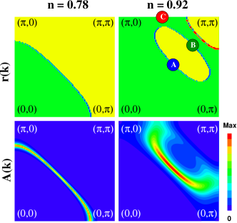
Figure 2: Renormalized energy, $r({\bf k})$, (upper panels) and spectral function, $A({\bf k})$, (lower panels) for the 2D Hubbard model with $U=8t$ and $T=0$. The color code for the upper panels is: green ($r<0$), blue ($r=0$), yellow ($r>0$), red ($r\rightarrow\infty$).

In contrast, close to the Mott transition the short-range correlations become important and the off-diagonal components of the cluster self-energy become comparable with $\Sigma_{0}$. As a consequence, at zero frequency the denominators in Eq. (Fermi arcs and the hidden zeros of the Green’s function in the pseudogap state) may acquire opposite signs generating a divergence in the lattice self-energy. This pole of $\Sigma({\bf k},\omega=0)$, or equivalently of $r({\bf k})$, gives rise to a zero of the lattice Green’s function. We show in Fig. 2 the renormalized energy, $r({\bf k})$, and the spectral function $A({\bf k},\omega=0)=-1/\pi ImG({\bf k},0)$ for a two-dimensional Hubbard model with $U=8t$ at zero temperature for two values of doping. For $n=0.78$ (left panels) we have a large electron-type Fermi surface (blue line in the $r({\bf k})$ panel) separating the occupied region of the Brillouin zone (green), defined by $r({\bf k})<0$ from the unoccupied region (yellow) defined by $r({\bf k})>0$. The Fermi surface can be also traced in the $A({\bf k})$ panel as the maximum of the spectral function. On the other hand, for $n=0.92$ a qualitatively different picture emerges. The Fermi surface (blue line) is now represented by a hole pocket and, in addition, we have a line of zeros of the Green’s function (red line) close to the $(\pi,\pi)$ region of the Brillouin zone. Furthermore, there is no one-to-one correspondence between the Fermi surface and the maximum of the spectral function. This behavior has two origins: 1) the proximity of a zero line suppresses the weight of the quasiparticle on the far side of the pocket, and 2) for k-points corresponding to $r({\bf k})\neq 0$ the quasiparticles are pushed away from $\omega=0$ and a pseudogap opens at the Fermi level. We show this explicitly in Fig. 3 by comparing the low frequency dependence of the spectral function in three different points of the Brillouin zone, marked by A, B and C in Fig. 2. Notice the suppression of the zero frequency peak at point B and the frequency shift $\delta=-0.05t$ of the peak at point C. The cumulant approach provides a simple interpretation of this effect, observed in photo emission experimentsexper , in terms of the emergence of infinite self-energy lines or equivalently Luttinger lines ( lines of zeros of the Greens function).

In conclusion, our strong coupling CDMFT study of the Hubbard model shows that the lightly doped system is characterized by a small, closed Fermi line that appears in the zero frequency spectral function as an arc due to the presence of a line of zeros of the Green’s function near the “dark side” of the Fermi surface. These lines appear near the Mott insulator in order to satisfy the generalized Luttinger theoremdzy ,

$$\frac{N}{V}=2\int_{{\mbox{Re}}G({\bf k},\omega=0)>0}\frac{d^{2}{\bf k}}{(2\pi)^{2}}.$$ (14)

While this theorem is not exactly satisfied in our finite cluster calculation due to the small cluster approximation, even this small cluster size has all the qualitative elements needed to interpret the physics of the underdoped regime which is controlled by the position of the lines of zeros and infinities. Notice that the standard Luttinger theorem will be always violated in a system characterized by a pseudogap, and it is strongly violated in our solution as the area contained in the pockets shrinks. The tendency to increase the area contained by the Luttinger surface as the pockets shrink is correctly captured by our approximation. Furthermore, we identify the pseudogap which is seen in leading edge study of photo emission experiments as the small negative shift of the spectral weight in points of the Brillouin zone that are not on the Fermi line (for example point C in Fig. 2), which is distinct from the larger gap between the peaks above and below the Fermi level (see Fig. 3).

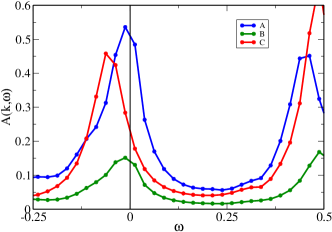
Figure 3: Frequency dependence of the spectral function for three points in the Brillouin zone marked by A, B, and C in Fig. 2.

Remarkably, the lines of poles of the self energy appear first far from the Fermi surface. This is a strong coupling instability which has no weak coupling precursors on the Fermi surface. Our results raise an interesting question. If the evolution in Figure 2 from large to small doping is continuous, it has to go through a critical point where the topology of the Fermi surface (and perhaps that of the lines where the self energy is infinite) changes. This topological change and its possible connection to an underlying critical point at finite doping in the cuprate phase diagram deserves further investigation.

ACKNOWLEDGMENTS: This research was supported by the NSF under grant DMR-0096462 and by the Rutgers University Center for Materials Theory. Many useful discussions with M. Civelli, B. Kyung, A. M. Tremblay, M. Capone, O. Parcollet and A. Tsvelik are gratefully acknowledged. Special thanks to K. Haule and M. Civelli for allowing the use of their ED and NCA programs.

References

- (1) T. Timusk and B Statt, Rep. Prog. Phys. 62, 61 (1999).
- (2) A. Georges, G. Kotliar, W. Krauth, and M. J. Rozenberg, Rev. Mod. Phys. 68, 13 (1996).
- (3) T. Maier, M. Jarrel, T. Pruschke and J. Keller, Eur. Phys. J. B 13, 613 (2000); M. Jarrel, T. Maier, M. H. Hettler, and A. N. Tahvildar-Zadeh, Europhys. Lett. 56, 563 (2001); T.D. Stanescu and P. Philips, Phys. Rev. Lett. 91, 017002 (2003); D. Sénéchal and A.-M.S. Tremblay, Phys. Rev. Lett. 92, 126401 (2004); B. Kyung, S.S. Kancharla, D. Sénéchal, A.-M.S. Tremblay, M. Civelli, and G. Kotliar, cond-mat/0502565 (2005).
- (4) T.D. Stanescu and G. Kotliar, Phys. Rev. B 70, 205112 (2004).
- (5) G. Kotliar, S.Y. Savrasov, G. Palsson, and G. Biroli, Phys. Rev. Lett. bf 87, 186401 (2001).
- (6) F.H.L. Essler and A.M. Tsvelik, Phys. Rev. B 65, 1151171 (2002).
- (7) D. Sénéchal, D. Perez, and M. Pioro-Ladrière, Phys. Rev. Lett. 84, 522 (2000).
- (8) G. Biroli, O. Parcollet, and G. Kotliar, Phys. Rev. B 69, 205108 (2004).
- (9) S. Biermann, A. Georges, A. Lichtenstein, and T. Giamarchi, Phys.Rev.Lett 87, 276405 (2001).
- (10) M. Capone, M. Civelli, S.S. Kancharla, C. Castellani, and G. Kotliar, Phys. Rev. B 69, 195105 (2004).
- (11) M. Civelli, M. Capone, S.S. Kancharla, O. Parcollet, and G. Kotliar, cond-mat/0411696.
- (12) D.S. Marshall et al., Phys. Rev Lett. 76, 4841 (1996); M.R. Norman et al., Nature 392, 157 (1998); A. Damascelli, Z.X. Shen, and Z. Hussain, Rev. Mod. Phys. 75, 473 (2003).
- (13) I. Dzyaloshinskii, Phys. Rev. B 68, 085113 (2003).