Electron and spin correlations in semiconductor heterostructures: Quantum Singwi-Tosi-Land-Sjölander theory

Abstract

We apply the quantum Singwi-Tosi-Land-Sjölander (QSTLS) theory for a study of many-body effects in the quasi-two-dimensional (Q2D) electron liquid (EL) in $GaAs/Al_{x}Ga_{1-x}As$ heterojunctions. The effect of the layer thickness is included through a variational approach. We have calculated the density, spin-density static structure factors, spin-dependent pair distribution functions (PDF) and compared our results with those of two-dimensional (2D) EL given in earlier papers. Using the static structure factors (SSF) we have calculated various dynamic correlation functions such as spin-dependent local-field factors (LFF) and effective potentials of the Q2D EL. We have also calculated the inverse static dielectric function of the 2D and Q2D EL using different approximations. We find that the effect of finite thickness on the dielectric function is remarkable and at the intermediate values of wave number $q$ there is a significant difference between the QSTLS and STLS results.

I Introduction

During the last decades quasi-two-dimensional electron systems have been of considerable interest because of technological relevance to high-mobility electronic devices. Many authors have investigated Q2D systems applying various methods AFS and most of the theoretical calculations have been performed in the framework of the random phase approximation (RPA). However, it is well-known that the RPA neglects the Pauli and Coulomb hole surrounding each particle and is not satisfactory approximation at low densities MH . Therefore a number of authors have studied beyond-RPA effects by including the static LFF such as in the Singwi-Tosi-Land-Sjölander (STLS) approach STLS68 . A common viewpoint is the need to incorporate dynamic correlations and the importance of dynamic LFF is evidence. The dynamic LFF has been introduced in several works via different schemes ST . One of these works is that of Hasegawa and Shimizu using the Wigner distribution function HS . The approach is usually named as the quantum STLS and has been applied to 2D EL by Moudgil and coworkers MAP . Their calculations have been generalized in our recent work KS to the more realistic case of electrons in Q2D semiconducting heterostructures investigated by Bulutay and Tomak (BT) BT . The aim of this work is to extend our previous investigations to include both electron and spin correlations.

The outline of this paper is as follows. In Sec. II, we discuss briefly the theoretical formalism of the self-consistent QSTLS equations applied to the Q2D EL in GaAs/Al_xGa_1-xAs heterojunctions based on the variational approach proposed by Bastard BA . In Sec. III the results and discussion are given, and in Sec. IV we summarize the main results and gather our assessment of the performance of the QSTLS for semiconductor heterostructures.

II Theory

We consider a GaAs/Al_xGa_1-xAs heterojunction where the electrons move into the GaAs side and form 2D subbands. For an accurate account of the electronic distribution we use Bastard’s variational approach given in BT’s work, where the electron effective masses $m_{A,B}$ and dielectric constants $\varepsilon$_A,B are considered to be different in the GaAs and Al_xGa_1-xAs layers. In the regime where only the lowest subband is populated the self-consistent equations for density and spin-density static structure factors at zero-temperature can be written as MAP

$$\chi^{d}\left({q,\omega}\right)=\frac{\chi_{0}\left({q,\omega}\right)}{1-V\left(q\right)\left[{1-G\left({q,\omega}\right)}\right]\chi_{0}\left({q,\omega}\right)}$$

$$S\left(q\right)=-\frac{2\hbar}{n}\int\limits_{0}^{\infty}{Im\left[{\chi^{d}\left({q,\omega}\right)}\right]d\omega}$$

$$G\left({q,\omega}\right)=-\frac{1}{n}\int{\frac{V(q^{\prime})}{V(q)}\frac{\chi_{0}\left({\vec{q},\vec{{q}^{\prime}};\omega}\right)}{\chi_{0}\left({\vec{q},\omega}\right)}\left[{S\left({\left|{\vec{q}-\vec{{q}^{\prime}}}\right|}\right)-1}\right]\frac{d\vec{{q}^{\prime}}}{\left({2\pi}\right)^{2}}}$$

$$\chi^{S}\left({q,\omega}\right)=-g^{2}\mu_{B}^{2}\frac{\chi_{0}\left({q,\omega}\right)}{1-V\left(q\right)J(q,\omega)\chi_{0}\left({q,\omega}\right)}$$

$$\tilde{S}\left(q\right)=\frac{\hbar}{2\pi ng^{2}\mu_{B}^{2}}\int\limits_{-\infty}^{\infty}{Im\left[{\chi^{S}\left({q,\omega}\right)}\right]d\omega}$$

$$J\left({q,\omega}\right)=\frac{1}{n}\int{\frac{V(q^{\prime})}{V(q)}\frac{\chi_{0}\left({\vec{q},\vec{{q}^{\prime}};\omega}\right)}{\chi_{0}\left({\vec{q},\omega}\right)}\left[{\tilde{S}\left({\left|{\vec{q}-\vec{{q}^{\prime}}}\right|}\right)-1}\right]\frac{d\vec{{q}^{\prime}}}{\left({2\pi}\right)^{2}}}$$

where

$$\chi_{0}\left({\vec{q},\vec{{q}^{\prime}};\omega}\right)=-\frac{2}{\hbar}\int{\frac{d\vec{p}}{h^{2}}\frac{f^{0}\left({\vec{p}+\raise 3.01385pt\hbox{${\hbar\vec{{q}^{\prime}}}$}\!\mathord{\left/{\vphantom{{\hbar\vec{{q}^{\prime}}}2}}\right.\kern-1.2pt}\!\lower 3.01385pt\hbox{$2$}}\right)-f^{0}\left({\vec{p}-\raise 3.01385pt\hbox{${\hbar\vec{{q}^{\prime}}}$}\!\mathord{\left/{\vphantom{{\hbar\vec{{q}^{\prime}}}2}}\right.\kern-1.2pt}\!\lower 3.01385pt\hbox{$2$}}\right)}{\omega-\raise 3.01385pt\hbox{${\vec{q}\vec{p}}$}\!\mathord{\left/{\vphantom{{\vec{q}\vec{p}}m}}\right.\kern-1.2pt}\!\lower 3.01385pt\hbox{$m$}+i0}}$$

with $f^{0}\left(\vec{p}\right)$ is the Fermi – Dirac distribution function, $\chi_{0}\left({\vec{q};\omega}\right)=\chi_{0}\left({\vec{q},\vec{q};\omega}\right)$ is the free-electron response function and

$$V\left(q\right)=\frac{2\pi e^{2}}{q\bar{\varepsilon}}F\left(q\right)$$

is the Fourier transform of the effective potential. Here $F(q)$ is the form factor to the Coulomb interaction due to the layer thickness given in the BT’s work and $\bar{\varepsilon}$= ($\varepsilon$_A+$\varepsilon$${}_{B})/2$ is the average dielectric constant. A strictly 2D electron gas with $\delta$-function density distribution is obtained by setting $F(q)$ = 1 in Eq. (5). To solve the sets of Eqs. (1a-3a) and (1b-3b) we have used the procedure proposed by de Freitas et al. FIS and obtained the following self-consistent equations

$$S\left(q\right)=\frac{q^{2}k_{F}}{\pi^{2}n}\int\limits_{0}^{\gamma\left(q\right)}f\ \left(q,\beta\right)d\beta$$

$$G\left({q,\beta}\right)=-\frac{1}{\left({2\pi}\right)^{2}n}\int\limits_{0}^{\infty}{dq^{\prime}\int\limits_{0}^{2\pi}{d\phi\mbox{ }h\left({\vec{q},\vec{q}^{\prime};\beta}\right)\left[{S\left({q^{\prime}}\right)-1}\right]}}$$

$$\tilde{S}\left(q\right)=\frac{q^{2}k_{F}}{\pi^{2}n}\int\limits_{0}^{\gamma\left(q\right)}{\tilde{f}\left({q,\beta}\right)d\beta}$$

$$J\left({q,\beta}\right)=\frac{1}{\left({2\pi}\right)^{2}n}\int\limits_{0}^{\infty}{d{q}^{\prime}\int\limits_{0}^{2\pi}{d\phi\mbox{ }h\left({\vec{q},\vec{{q}^{\prime}};\beta}\right)\left[{\tilde{S}\left({q}^{\prime}\right)-1}\right]}}$$

with

$$f\left(q,\beta\right)=\left({\sqrt{1-\frac{q^{2}\sin^{2}\beta}{4k_{F}^{2}}}+\frac{\cot^{2}\beta}{\sqrt{1-\frac{q^{2}\sin^{2}\beta}{4k_{F}^{2}}}}}\right)\frac{\left({1-\cos\beta}\right)}{q+\frac{m}{\pi\hbar^{2}}qV\left(q\right)\left[{1-G\left({q,\beta}\right)}\right]\left({1-\cos\beta}\right)},$$

$$\tilde{f}\left({q,\beta}\right)=\left({\sqrt{1-\frac{q^{2}\sin^{2}\beta}{4k_{F}^{2}}}+\frac{\cot^{2}\beta}{\sqrt{1-\frac{q^{2}\sin^{2}\beta}{4k_{F}^{2}}}}}\right)\frac{\left({1-\cos\beta}\right)}{q+\frac{m}{\pi\hbar^{2}}qV\left(q\right)J\left({q,\beta}\right)\left({1-\cos\beta}\right)}\quad,$$

$$\gamma\left(\rho\right)=\left\{{\begin{array}[]{l}\pi\mathord{\left/{\vphantom{\pi 2}}\right.\kern-1.2pt}2\mbox{ },q\leq 2k_{F}\\ \mbox{sin}^{-1}\left({\raise 3.01385pt\hbox{${2k_{F}}$}\!\mathord{\left/{\vphantom{{2k_{F}}q}}\right.\kern-1.2pt}\!\lower 3.01385pt\hbox{$q$}}\right)\mbox{ },q>2k_{F}\\ \end{array}}\right.$$

$$h\left({\vec{q},\vec{q}^{\prime};\beta}\right)=\frac{q^{\prime}\left[{1-r\left({\vec{q},\vec{q}-\vec{q}^{\prime};\beta}\right)}\right]\left({q-q^{\prime}\cos\phi}\right)}{q(1-\cos\beta)}\frac{V\left({\sqrt{q^{2}+q^{\prime 2}-2qq^{\prime}\cos\phi}}\right)}{V\left(q\right)}$$

where $r(\vec{q},\vec{q}-\vec{q}^{\prime};\beta)$ is the positive root of the following equation

$$\left[{\frac{\vec{q}.\left({\vec{q}-\vec{q}^{\prime}}\right)}{\vec{q}^{2}}}\right]^{2}=\frac{1}{1-r^{2}}\frac{4k_{F}^{2}}{\vec{q}^{2}}-\frac{1}{r^{2}}\left({\frac{4k_{F}^{2}}{q^{2}\sin^{2}\beta}-1}\right)\cos^{2}\beta\quad.$$

Here $n$, $k_{F}=\sqrt{2\pi{\kern 1.0pt}n}$ and $\phi$ are the electron density, Fermi wave number and angle between $\vec{q}$ and $\vec{q}^{\prime}$, respectively MAP . Using the integration by parts we can write the density and spin-density static structure factors as

$$S\left(q\right)=\frac{2q^{2}}{\pi}\int\limits_{0}^{\gamma\left(q\right)}{\cot\beta\sqrt{1-\frac{q^{2}\sin^{2}\beta}{4}}\frac{q\sin\beta+\sqrt{2}r_{S}F\left(q\right)(1-\cos\beta)^{2}\frac{\partial G\left({q,\beta}\right)}{\partial\beta}}{\left({q+\sqrt{2}r_{S}F\left(q\right)\left[{1-G\left({q,\beta}\right)}\right]\left({1-\cos\beta}\right)}\right)^{2}}}d\beta\quad,$$

$$\tilde{S}\left(q\right)=\frac{2q^{2}}{\pi}\int\limits_{0}^{\gamma\left(q\right)}{\cot\beta\sqrt{1-\frac{q^{2}\sin^{2}\beta}{4}}\frac{q\sin\beta-\sqrt{2}r_{S}F\left(q\right)(1-\cos\beta)^{2}\frac{\partial J\left({q,\beta}\right)}{\partial\beta}}{\left({q+\sqrt{2}r_{S}F\left(q\right)J\left({q,\beta}\right)\left({1-\cos\beta}\right)}\right)^{2}}}d\beta$$

These forms of the structure factors are appropriate for the numerical integration because the integrands remain finite in the limit $\beta\to 0$.

III Results and discussions

In our recent paper KS we have solved the equations (6a-7a) for 2D and Q2D electron liquids in semiconductor heterojunctions. In the case of 2D EL we have obtained the SSF and PDF in good agreement with Monte Carlo results. In this paper we solve the equations (6b-7b) for the Q2D electron liquid in GaAs/Al_xGa_1-xAs heterojunctions having a step-barrier potential with $U_{b}=$0.3eV , $\varepsilon$${}_{A}=$13, $\varepsilon$_B = 12.1, $m_{A}=$0.07$m_{e}$ and $m_{B}=$0.088$m_{e}$ , where $m_{e}$ is the vacuum mass of the electron BT . Using the obtained results we calculate the spin-dependent pair-correlation functions, dynamic local-field factors, spin-dependent effective potentials, inverse static dielectric function and compare our results with those given in Refs.7 and 8.

III.1 Static spin-density structure factors

The static structure factor $S(q)$ of the 2D EL was shown in Fig. 1 of our recent paper KS . In this work we have calculated the spin-density SSF $\tilde{S}(q)$ of 2D and Q2D EL by solving the Eqs. (6b) and (7b) in the self-consistent way for several values of electron density and the results are shown in Fig. 1. It is seen that in the case of 2D EL our results are similar to those of Ref. 6 and the effect of the layer thickness is remarkable for a wide range of electron densities.

III.2 Spin-dependent electron pair-correlation functions

The spin-symmetric and spin-antisymmetric electron pair-correlation functions can be expressed as

$$g_{\uparrow\uparrow}\left(r\right)=0.5\;\left[{g\left(r\right)+\tilde{g}\left(r\right)}\right]$$

$$g_{\uparrow\downarrow}\left(r\right)=0.5\;\left[{g\left(r\right)-\tilde{g}\left(r\right)}\right]$$

where

$$g\left(r\right)=1+\int\limits_{0}^{\infty}{qJ_{0}\left({qr}\right)\left[{S\left(q\right)-1}\right]dq}$$

$$\tilde{g}\left(r\right)=\int\limits_{0}^{\infty}{qJ_{0}\left({qr}\right)\left[{\tilde{S}\left(q\right)-1}\right]dq}$$

To study the effect of electron density we show in Fig. 2. the spin-dependent PDF $g_{\downarrow\uparrow}(r)$ of 2D EL for different values of density parameter $r_{s}.$ We observe that our PDFs differ from those of Moudgil and coworkers at small values of $r$. This difference in the behavior of PDFs stems from the incorrect results of Moudgil and coworkers for the SSF at large $q^{\prime}s$ discussed in our previous paper KS .

To study the effect of the layer thickness on PDFs we have calculated the spin-dependent electron pair-correlation functions $g_{\downarrow\downarrow}(r)$ of 2D and Q2D EL for different values of electron density parameter $r_{s}.$ We find that $g_{\downarrow\downarrow}(r)$ is almost independent of $r_{s}$ and is therefore plotted in Fig. 3 only for $r_{s}=3.$ We observe from the figure that the effect of the layer thickness is considerable for an intermediate region of the inter-particle distance.

III.3 Spin-symmetric and spin-antisymmetric dynamic local-field factors:

To compare our results with those of Moudgil et al. and to study the effect of the layer thickness we show in Figs. 4 and 5 the spin-dependent dynamic LFFs of 2D and Q2D EL as a function of $\omega$ for $q=$ 1.1$k_{F}$ and $r_{s}=$ 3. We observe that our results for 2D EL are similar to those given in Ref.6 and the layer thickness has a remarkable influence on G(q,$\omega)$ and J(q,$\omega)$ for a wide range of frequencies $\omega$.

III.4 Effective dynamic potentials

Spin-symmetric and spin-antisymmetric dynamic effective potentials can be calculated from the spin-symmetric and spin-antisymmetric dynamic LFF as

$$V_{eff}^{s}\left({q,\omega}\right)=V\left(q\right)\left[{1-G\left({q,\omega}\right)}\right]$$

$$V_{eff}^{a}\left({q,\omega}\right)=V\left(q\right)J(q,\omega)$$

The effective potentials of the 2D and Q2D EL obtained in the static limit ( i.e., $\omega$ = 0) for $r_{s}$ = 1 and 3 are shown Figs. 6 and 7. We observe remarkable differences in the results of 2D and Q2D EL for all values of $q$ and $r_{s}.$ We note that because of incorrect results for the SSF given in Ref. 6 our results for both spin-symmetric and spin-antisymmetric static effective potentials of 2D EL differ considerably from those of Moudgil and coworkers in the region of large values of $q\quad(q>$3.5$q_{F}$).

Following the authors of Ref.6 we define the spin-dependent effective dynamic potential as

$$V_{eff\uparrow\uparrow}=V_{eff}^{s}\left({q,\omega}\right)+V_{eff}^{a}\left({q,\omega}\right)$$

$$V_{eff\uparrow\downarrow}=V_{eff}^{s}\left({q,\omega}\right)-V_{eff}^{a}\left({q,\omega}\right)$$

The real and imaginary spin-dependent effective dynamic potentials of 2D and Q2D EL for $r_{s}$ = 1 and $q=$1.1$k_{F}$ are plotted, respectively, in Figs. 8 and 9. It is seen from the figures that the effect of layer thickness is significant for a wide range of frequency $\omega$ and our results for 2D EL are similar to those of Moudgil and co-workers MAP . We note that the values of the real spin-dependent effective dynamic potentials shown in the Fig. 9(a) of Ref.6 is not correct. By using the values of $V_{eff}^{s}\left({q,\omega}\right)$ and $V_{eff}^{a}\left({q,\omega}\right)$ at $\omega$ = 0 we can see that the authors of Ref.6 have divided the correct values of $V_{eff\uparrow\uparrow}(q,\omega)$ and $V_{eff\uparrow\uparrow}(q,\omega)$ by 2.

III.5 Inverse static dielectric function

Finally, we calculate the inverse static dielectric function of 2D and Q2D EL for $r_{s}=$3 using different approximations. The figure 10 shows that the QSTLS results differ less from those of the STLS approximation in the Q2D EL than in the 2D EL. However, at the intermediate values of $q$ there is a significant difference between the QSTLS and STLS results.

IV Conclusions

Using the QSTLS approximation we have studied the electron and spin correlations in GaAs/Al_xGa_1-xAs heterojunctions. We have calculated the spin-dependent PDF, SSF, dynamic LFF, effective potential and inverse static dielectric function of 2D and Q2D EL. We have shown that the results for Q2D EL in semiconductor heterostructures differ remarkably from those of 2D EL and the difference between the QSTLS and the STLS results of Q2D EL is considerable. It is hoped that our results will be of help in investigating the effect of electron and spin correlations on properties of Q2D electron systems.

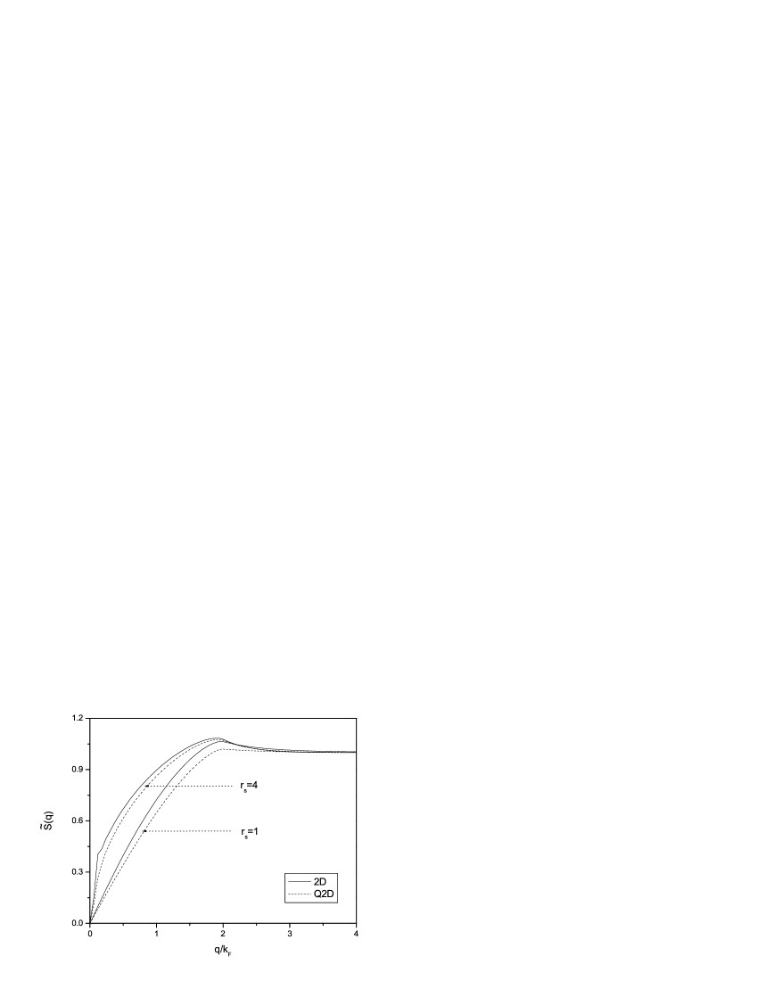
Figure 1: Static spin-density structure factors for $r_{s}=$1, 2, 3 and 4.

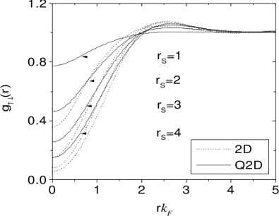
Figure 2: Spin-dependent pair-correlation functions $g_{\downarrow\uparrow}(r)$ for $r_{s}=$1, 2, 3 and 4.

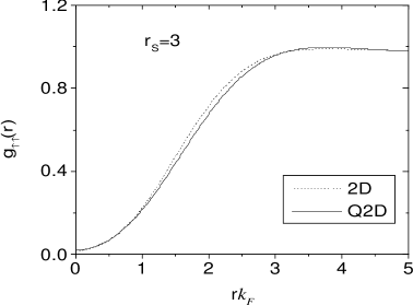
Figure 3: Spin-dependent pair-correlation functions $g_{\downarrow\downarrow}(r)$ of the 2D and Q2D EL for $r_{s}=$3.

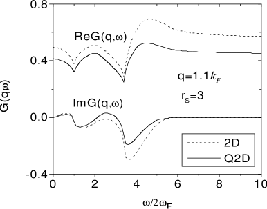
Figure 4: Spin-symmetric dynamic structure factors for $r_{s}$ = 3 and $q=$1.1$k_{F}.$

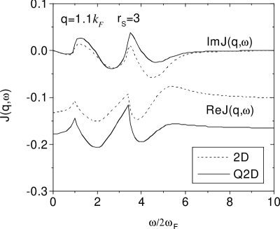
Figure 5: Spin-antisymmetric dynamic structure factors for $r_{s}$ = 3 and $q=$1.1$k_{F}.$

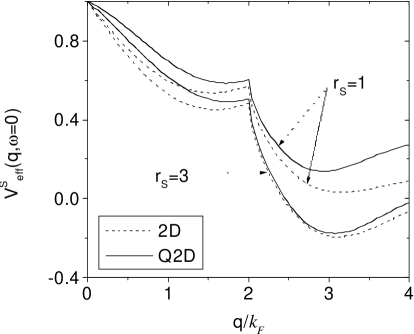
Figure 6: Static spin-symmetric effective potentials for $r_{s}$ = 1 and 3.

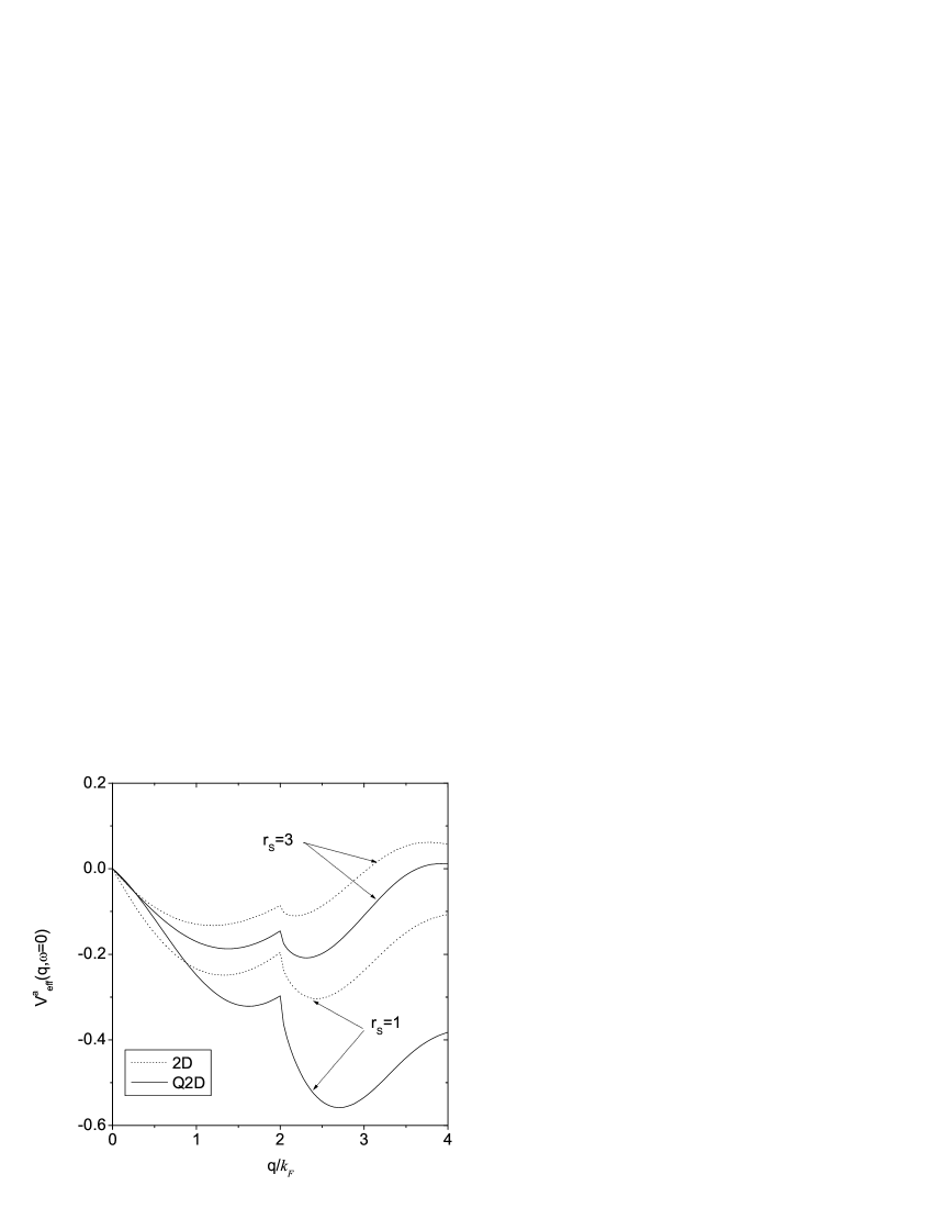
Figure 7: Static spin-antisymmetric effective potentials for $r_{s}$ = 1 and 3.

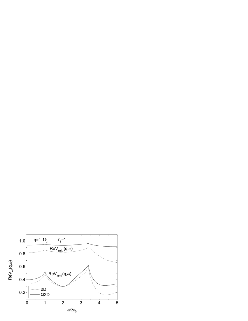
Figure 8: Real spin-dependent effective dynamic potentials $r_{s}$ = 1 and $q=$1.1$k_{F}$.

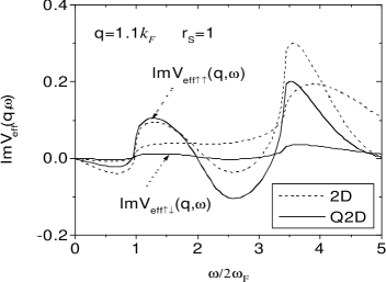
Figure 9: Imaginary spin-dependent effective dynamic potentials $r_{s}$ = 1 and $q=$1.1$k_{F}$.

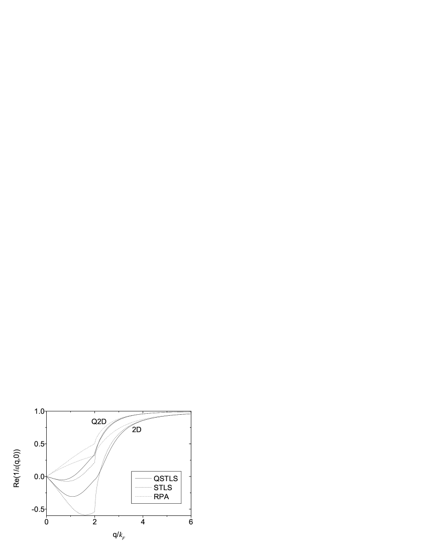
Figure 10: Inverse static dielectric function of 2D and Q2D EL for $r_{s}=$3.

References

(1)
T. Ando, A.B. Fowler, and F. Stern, Rev. Mod. Phys. 54 ,
437 (1982).
(2)
G.D. Mahan, Many-Particle Physics, 2nd ed. (Plenum
Press, New York , 1990).
(3)
K. S. Singwi, M. P. Tosi, R. H. Land , and A. Sjölander,
Phys.Rev.176 , 589 (1968).
(4)
K.S. Singwi and M.P. Tosi, in Solid State Physics, edited by H. Ehrenreich, F. Seitz, and D.Turnbull
(Academic, New York , 1981), Vol. 36, p.177.
(5)
T.Hasegawa and M.Shimizu, J.Phys.Soc.Jpn. 38 , 965 (1975).
(6)
R.K. Moudgil , P.K. Ahluwalia, and K.N. Pathak, Phys. Rev. B
52 , 11945 (1995).
(7)
Nguyen Quoc Khanh and Nguyen Thanh Son, Physica B 344 , 176
(2004)
(8)
C.Bulutay and M.Tomak , Phys. Rev. B 54 , 14643 (1996).
(9) G. Bastard,
Wave Mechanics Applied to Semiconductor Heterostructures (Les Editions de Physique, Les Ulis Cesex, 1988) p.155.
(10)
U. de Freitas, L.C. Ioriatti , and N. Studart, J. Phys. C
20 , 5983 (1987).