Relaxation in a glassy binary mixture: Comparison of the mode-coupling theory to a Brownian dynamics simulation

Abstract

We solved the mode-coupling equations for the Kob-Andersen binary mixture using the structure factors calculated from Brownian dynamics simulations of the same system. We found, as was previously observed, that the mode-coupling temperature, $T_{c}$, inferred from simulations is about two times greater than that predicted by the theory. However, we find that many time dependent quantities agree reasonably well with the predictions of the mode-coupling theory if they are compared at the same reduced temperature $\epsilon=(T-T_{c})/T_{c}$, and if $\epsilon$ is not too small. Specifically, the simulation results for the incoherent intermediate scattering function, the mean square displacement, the relaxation time and the self-diffusion coefficient agree reasonably well with the predictions of the mode-coupling theory. We find that there are substantial differences for the non-Gaussian parameter. At small reduced temperatures the probabilities of the logarithm of single particle displacements demonstrate that there is hopping-like motion present in the simulations, and this motion is not predicted by the mode-coupling theory. The wave vector dependent relaxation time is shown to be qualitatively different than the predictions of the mode-coupling theory for temperatures where hopping-like motion is present.

I Introduction

The mode-coupling theory Goetze ; Das has been used extensively to describe the slow relaxation observed in supercooled liquids close to the glass transition. The qualitative predictions of the theory have been compared to experiments Das ; Lunkenheimer and simulations Barrat ; KobAndersen ; Fuchs ; Franosch . However, until recently, quantitative comparisons which include wave vector dependence and use exact (i.e. obtained from simulations) static information have been rare Nauroth ; KobNauroth ; Foffi .

Nauroth and Kob Nauroth compared the non-ergodicity parameters predicted by the mode-coupling theory to Newtonian dynamics simulations of a binary Lennard-Jones mixture. They used the structure factors determined from the simulations as the input to the mode-coupling theory, and found that the transition temperature predicted by the theory was approximately twice higher than the transition temperature inferred from simulations. However, the non-ergodicity parameters predicted by the theory agreed reasonably well with the ones determined from simulations. In a later work, Kob, Nauroth, and Sciortino KobNauroth quantitatively compared the shape of the intermediate scattering functions predicted by the mode-coupling theory to results of Newtonian dynamics simulations. Since the transition temperature predicted by the theory is greater than that inferred from simulations, the intermediate scattering functions at the same temperature (and close to the transition temperature) are vastly different. Therefore, the authors compared scattering functions predicted by the theory at a higher temperature to scattering functions obtained from simulations at a lower temperature. The two corresponding temperatures were determined by the requirement that the relaxation time be the same for one wave vector around the first peak in partial structure factor for the larger particles. Once the two corresponding temperatures where fixed, the authors showed that for a few wave vectors the shape of the incoherent intermediate scattering function was well described by the mode-coupling theory. Also, Foffi et al. Foffi compared simulation results to the mode-coupling theory for mixtures of hard spheres. They found that, if the time scale is rescaled, the mode-coupling theory accurately predicts the shape of the intermediate scattering functions in the $\alpha$ relaxation region.

Recently, the mode-coupling theory has been compared to molecular and Brownian dynamics simulations of polydisperse spheres with a strong repulsive core by Voigtmann, Puertes, and Fuchs Voigtmann . They used the Percus-Yevick theory to determine the structure factors for the mode-coupling theory calculations. For the comparison of the theory with simulation, they adjusted the packing fraction and allowed a “dynamical” length scale to vary slightly. They found that after these adjustments the intermediate scattering functions and the mean square displacement predicted by the mode-coupling theory agreed well with the simulation results.

The goal of the work presented here is to compare the predictions of the mode coupling theory to the results of Brownian dynamics simulations using the smallest possible number of adjustable parameters. In other words, we would like to test the predictive power of the mode-coupling theory rather than demonstrate that by making a number of parameters adjustable, we can reproduce the simulation results very accurately. In view of the difference between the mode-coupling transition temperature predicted by the theory and inferred from simulations, a minimalistic approach is to compare theoretical predictions and results of the simulations at the same reduced temperature $\epsilon=(T-T_{c})/T_{c}$. Briefly, the result of our comparison is that many time dependent quantities predicted by the theory agree reasonably well with results of the simulations if $\epsilon$ is not too small. However, there is significant disagreement between the theoretical predictions and the simulation results for the non-Gaussian parameter for all but the highest reduced temperatures. Finally, at low reduced temperatures there is a hopping-like motion present in the simulations which is not predicted by the mode-coupling theory.

One of the reasons for testing the mode coupling theory against Brownian dynamics simulations is that the approximations involved in this theory applied to Brownian systems are somewhat less severe. The first approximation of the theory, projecting stress fluctuations onto the subspace of the density products Goetze , is exact for Brownian systems. However, the main and the most drastic approximation of the mode coupling theory, the self-consistent factorization approximation, has to still be used. The present study shows explicitly that it is the factorization approximation that is responsible for the failure of the mode coupling theory for low reduced temperatures.

The paper is organized as follows. In section II we briefly describe the Brownian dynamics simulations. In section III we describe the mode-coupling equations which are appropriate for a binary mixture evolving with Brownian dynamics, and briefly present the mode-coupling calculation (the method is described in detail in the appendix). In section IV we describe the method used to find the transition temperature from the mode-coupling theory, and briefly discuss the non-ergodicity parameters. We compare the intermediate scattering functions in section V and the mean square displacement in section VI. We compare the non-Gaussian parameter in section VII, and the probability distribution of the logarithm of single particle displacements in section VIII. We discuss the results in section IX.

II Brownian Dynamics Simulations

We simulated a system consisting of $N_{A}=800$ particles of type A and $N_{B}=200$ particles of type B that was first considered by Kob and Andersen KobAndersen . The interaction potential is $V_{\alpha\beta}(r)=4\epsilon_{\alpha\beta}[({\sigma_{\alpha\beta}}/{r})^{12}-({\sigma_{\alpha\beta}}/{r})^{6}]$, where $\alpha,\beta\in\{A,B\}$, $\epsilon_{AA}=1.0$, $\sigma_{AA}=1.0$, $\epsilon_{AB}=1.5$, $\sigma_{AB}=0.8$, $\epsilon_{BB}=0.5$, and $\sigma_{BB}=0.88$. The simulations are performed with the interaction potential cut at $2.5\ \sigma_{\alpha\beta}$, and the box length of the cubic simulation cell is $9.4\ \sigma_{AA}$. Periodic boundary conditions were used.

We performed Brownian dynamics simulations. The equation of motion for the position of the $i_{th}$ particle of type $\alpha$, $\vec{r}\,_{i}^{\alpha}$, is

$$\dot{\vec{r}}\,_{i}^{\alpha}=\frac{1}{\xi_{0}}\vec{F}_{i}^{\alpha}+\vec{\eta}_{i}(t),$$ (1)

where the friction coefficient of an isolated particle $\xi_{0}=1.0$ and $\vec{F}_{i}^{\alpha}$ is the force acting on the $i_{th}$ particle of type $\alpha$,

$$\vec{F}_{i}^{\alpha}=-\nabla_{i}^{\alpha}\sum_{j\neq i}\sum_{\beta=1}^{2}V_{\alpha\beta}\left(\left|\vec{r}\,_{i}^{\alpha}-\vec{r}\,_{j}^{\beta}\right|\right)$$ (2)

with $\nabla_{i}^{\alpha}$ being the gradient operator with respect to $\vec{r}\,_{i}^{\alpha}$. In Eq. (1) the random noise $\vec{\eta}_{i}$ satisfies the fluctuation-dissipation theorem,

$$\left\langle\vec{\eta}_{i}(t)\vec{\eta}_{j}(t^{\prime})\right\rangle=2D_{0}\delta(t-t^{\prime})\delta_{ij}\mathbf{1}.$$ (3)

In Eq. (3), the diffusion coefficient $D_{0}=k_{B}T/\xi_{0}$ where $k_{B}$ is Boltzmann’s constant and $\mathbf{1}$ is the unit tensor. Since the equation of motion allows for diffusive motion of the center of mass, all the results will be presented relative to the center of mass (i.e. momentary positions of all the particles are always relative to the momentary position of the center of mass remark ). The results are presented in terms of the reduced units with $\sigma_{AA}$, $\epsilon_{AA}$, $\epsilon_{AA}/k_{B}$, and $\sigma_{AA}^{2}\xi_{0}/\epsilon_{AA}$ being the units of length, energy, temperature, and time, respectively. Since in these units the short-time self-diffusion coefficient is proportional to the temperature, in the comparisons with the mode-coupling theory the times are rescaled to $t^{*}=tD_{0}/\sigma_{AA}^{2}$.

The equations of motion, Eq. 1, were solved using a Heun algorithm with a small time step of $5\times 10^{-5}$. To save disk space, not all the generated configurations were saved to disk. Thus, the short time dynamics are not available at the lower temperatures. We simulated the temperatures $T=0.44$, 0.45, 0.47, 0.50, 0.55, 0.60, 0.80, 0.90, 1.0, 1.5, 2.0, 3.0, and 5.0. We ran equilibration runs and 4-6 production runs. The equilibration runs were typically twice shorter than the production runs, and the latter were up to $6\times 10^{8}$ time steps long for the lowest temperatures studied. The results presented are averages over the production runs.

III Mode-Coupling Theory

The mode-coupling theory leads to a set of integro-differential equations for the coherent intermediate scattering functions (i.e. dynamic partial structure factors),

$$S_{\alpha\beta}(q,t)=\left\langle\rho_{\vec{q}}^{\alpha}(t)\rho_{-\vec{q}}^{\beta}(0)\right\rangle$$ (4)

where

$$\rho_{q}^{\alpha}(t)=\frac{1}{\sqrt{N_{\alpha}}}\sum_{i=1}^{N_{\alpha}}e^{-\mathrm{i}\vec{q}\cdot\vec{r}\,_{i}^{\alpha}(t)}.$$ (5)

Note that the sum in Eq. (5) is taken over particles of type $\alpha$. The structure factors depend only on the magnitude of the wave vector $|\vec{q}\,|=q$. The time evolution of $\rho_{\vec{q}}^{\alpha}(t)$ for a system of interacting Brownian particles is governed by the adjoint Smoluchowski operator Nagele

$$\Omega=D_{0}\sum_{\alpha=1}^{2}\sum_{i=1}^{N_{\alpha}}\left[\nabla_{i}^{\alpha}-\beta\vec{F}_{i}^{\alpha}\right]\cdot\nabla_{i}^{\alpha}$$ (6)

where $\beta=1/k_{B}T$ and $D_{0}$ is the short time diffusion coefficient which is the same for both types of particles. We set $D_{0}=1.0$ for these calculations.

The mode-coupling equations governing the time evolution of the coherent intermediate scattering functions for Brownian mixtures have been derived by Nägele et al. Nagele1 :

$$\frac{\partial}{\partial t}\mathbf{S}(q,t) = -q^{2}D_{0}\>\mathbf{S}^{-1}(q)\>\mathbf{S}(q,t)$$

$$-\int_{0}^{t}\mbox{d}u\ \mathbf{M}(q,t-u)\frac{\partial}{\partial u}\mathbf{S}(q,u)$$

where

$$\mathbf{S}(q,t)=\begin{pmatrix}S_{AA}(q,t)&S_{AB}(q,t)\\ S_{BA}(q,t)&S_{BB}(q,t)\end{pmatrix},$$ (8)

is the matrix of coherent intermediate scattering functions, and $\mathbf{M}$ is the matrix of memory functions,

$$M_{\alpha\beta}(\vec{q},t) = \frac{VD_{0}}{32\pi^{2}\sqrt{N_{\alpha}N_{\beta}}}$$ (9)

$$\times\sum\limits_{l,l^{\prime},m,m^{\prime}}\int\mathrm{d}\vec{k}V_{\alpha lm}(\vec{q},\vec{k})V_{\beta l^{\prime}m^{\prime}}(\vec{q},\vec{k})$$

$$\times\ S_{mm^{\prime}}(|\vec{q}-\vec{k}|,t)S_{ll^{\prime}}(k,t)$$

where the vortex

$$V_{\alpha lm}(\vec{q},\vec{k}) = \frac{\vec{q}\cdot\vec{k}}{q}\delta_{\alpha m}C_{\alpha l}(k)$$ (10)

$$+\frac{\vec{q}\cdot(\vec{q}-\vec{k})}{q}\delta_{\alpha l}C_{\alpha m}(|\vec{q}-\vec{k}|).$$

In Eq. (10) the matrix $\mathbf{C}(q)$ is defined through the Ornstein-Zernike matrix equation

$$\mathbf{S}^{-1}(q)=\mathbf{1}-\mathbf{C}(q),$$ (11)

where $\mathbf{1}$ is the unit tensor. The mode-coupling theory equations allows one to calculate the time evolution of $S_{\alpha\beta}(q,t)$ with only the time independent quantity $S_{\alpha\beta}(q)=S_{\alpha\beta}(q,0)$ as an input.

The incoherent intermediate scattering functions

$$F_{\alpha}^{s}(q,t)=\left\langle e^{\mathrm{i}\vec{q}\cdot\left[\vec{r}\,_{i}^{\alpha}(t)-\vec{r}\,_{i}^{\alpha}(0)\right]}\right\rangle$$ (12)

are calculated using as input the coherent intermediate scattering function and the partial structure factors. Nägele et al. Nagele1 derived the equations governing the time evolution of $F_{\alpha}^{s}(q,t)$ for Brownian mixtures,

$$\frac{\partial}{\partial t}F_{\alpha}^{s}(q,t) = -q^{2}D_{0}F_{\alpha}^{s}(q,t)$$ (13)

$$-\int_{0}^{t}\mbox{d}uM_{\alpha}^{s}(q,t-u)\frac{\partial}{\partial u}F_{\alpha}^{s}(q,u)$$

where the memory function

$$M_{\alpha}^{s}(q,t) = \frac{D_{0}V}{\left(2\pi\right)^{2}N_{\alpha}}\int\mbox{d}\vec{k}\left(\frac{\vec{q}\cdot\vec{k}}{q}\right)^{2}F_{\alpha}^{s}(|\vec{q}-\vec{k}|)$$ (14)

$$\times\sum_{\delta\delta^{\prime}}C_{\alpha\delta}(k)S_{\delta\delta^{\prime}}(k,t)C_{\alpha\delta^{\prime}}(k)$$

For short times the integrals involving the memory function in Eqs. (LABEL:coheq) and (13) are approximately zero, therefore

$$\mathbf{S}(q,t)\approx\exp\left[-q^{2}D_{0}\,\mathbf{S}^{-1}(q)\,t\right]\,\mathbf{S}(q),$$ (15)

$$F_{\alpha}^{s}(q,t)\approx\exp\left[-q^{2}D_{0}t\right].$$ (16)

In Eq. (16) we used $F_{\alpha}^{s}(q,0)=1.0$.

According to Eqs. (15-16), at short times the particles undergo diffusive motion with a diffusion coefficient $D_{0}$. The effect of the memory function is to provide a feedback mechanism which produces a “caging” of the particles. For temperatures below the transition temperature $T_{c}$, there is structural arrest and the particles do not escape their cage. This results in a non-zero value of $\mathbf{S}(q,t)$ and $F_{\alpha}^{s}(q,t)$ as $t\rightarrow\infty$. For temperatures close to but above $T_{c}$, there is a plateau region in the log-log plot of the mean square displacement and the log-linear plot of the intermediate scattering functions. At long times the motion of the particles is again diffusive with a temperature dependent diffusion coefficient $D\ll D_{0}$.

We calculate the input to the mode-coupling equations, i.e. the partial static structure factors $S_{\alpha\beta}(q)$, directly from the Brownian dynamics simulations. Because of the finite size of the simulation box, the magnitude of the smallest wave vector calculated is $2\pi/L$, where $L$ is the length of the simulation box. We extrapolated $S_{\alpha\beta}(q)$ to zero by fitting the first few wave vectors to a polynomial. The method used to calculate the integrals of the memory functions require that the partial structure factors are known at equally spaced wave vectors (see the appendix for details on the numerical procedure implemented in this work). The structure factor for these wave vectors were determined by fitting the partial structure factors determined from the simulations to a cubic spline.

To solve the mode-coupling equations, we used 300 equally spaced wave vectors from $q=0$ to $q=40$ with the first wave vector $q_{0}=0.2/3$. We performed a few calculations with larger cutoffs for the integral and/or a finer grid of wave vectors. The difference in the values of the calculated intermediate scattering functions was at most 5% and less in most cases. This difference results in a less than 5% difference in the self-diffusion coefficient and the incoherent intermediate scattering function’s relaxation time.

The partial structure factors for temperatures which were not directly simulated were calculated by a quadratic polynomial interpolation between the points at three adjacent temperatures. For most interpolated temperatures, it is possible to use two different sets of temperatures to determine the structure factor at the interpolated temperature. Using different temperature ranges changed the value of $\mathbf{S}(q,t)$ by as much as 1%, but by less in most cases. At a few temperatures we also used a linear interpolation between two adjacent temperatures or a cubic interpolation using the four closest temperatures. The difference in the results were less than 2% using these different interpolation schemes. We conclude that the results depends little on the interpolation scheme.

First, we solved the mode-coupling equations for the coherent intermediate scattering functions until all the scattering functions decayed to zero or to a non-zero constant. Then the coherent scattering functions and the structure factor were used as the inputs for the calculation of the incoherent scattering functions, which were solved for the same times as for the coherent intermediate scattering functions.

Since the mode-coupling equations have to be solved for many decades in time, specialized techniques have been developed. We describe the method used to solve the mode-coupling equations in the appendix. The algorithm was first described by Fuchs et al. FuchsMCT , and then, in more detail, by Miyazaki, Bagchi and Yethiraj Miyazaki . It is an iterative technique which calculates the coherent and the incoherent scattering functions from $t=i\Delta t$ where $i\in\{N+1,\dots,2N\}$, assuming that the scattering functions are known for $t=j\Delta t$ where $j\in\{1,\dots,N\}$. Then the time step $\Delta t^{\prime}=2\Delta t$ is doubled, and the values of the scattering functions for $t=i\Delta t^{\prime}$ where $i\in\{1,\dots,N\}$ are determined from the values of the scattering functions for $t=j\Delta t$ where $j\in\{1,\dots,2N\}$. We begin the calculation for an initial time step of $10^{-8}$. For the first set of times, the scattering functions are not known. We used the approximation given by Eq. (15) and (16) to supply the values of the coherent and the incoherent scattering functions for the initial $N$ times. To check this approximation, we also used a more time consuming procedure to solve the mode-coupling equations for the initial $N$ times. In this procedure, the integrals of the memory function are included for $t>10^{-8}$. The difference in all calculated quantities was less than 0.5%.

IV Transition Temperature: Mode-Coupling Theory vs. Simulations

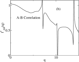
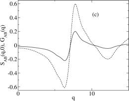
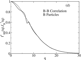
Figure 1: (a) Non-ergodicity parameter at $T_{c}$ for the A particles. Solid line: coherent correlator, A-A particles. Dashed line: incoherent correlator, A particles. (b) Non-ergodicity parameter at $T_{c}$: coherent correlator, A-B particles. (c) Dashed line: A-B partial structure factor, $S_{AB}(q)$. Solid line: $G_{AB}(q)=S_{AB}(q;t\rightarrow\infty)$ at $T_{c}$. (d) Non-ergodicity parameter at $T_{c}$ for the B particles. Solid line: coherent correlator, B-B particles. Dashed line: incoherent correlator, B particles.

The mode-coupling theory predicts an ergodicity breaking transition when $S_{\alpha\beta}(q,t\rightarrow\infty)\neq 0$ at some critical temperature $T_{c}$. To find the transition temperature we calculate $\mathbf{G}(q)=\lim_{t\rightarrow\infty}\mathbf{S}(q,t)$ as a function of temperature. We followed the procedure used in previous calculations of the non-ergodicity parameter BarratLatz ; Nauroth ; Barrat to calculate $\mathbf{G}(q)$. First, we took the Laplace transform of Eq. LABEL:coheq to get

$$\left[z+z\mathbf{M}(q,z)+q^{2}D_{0}\mathbf{S}^{-1}(q)\right]\mathbf{S}(q,z)=$$

$$\mathbf{S}(q)+\mathbf{M}(q,z)\mathbf{S}(q)$$

where $f(z)$ denotes the Laplace transform of $f(t)$, $f(z)=\int_{0}^{\infty}e^{-zt}f(t)$. To find the long time limit of $\mathbf{S}(q,t)$ we utilized the relationship $\lim_{t\rightarrow\infty}f(t)=\lim_{z\rightarrow 0}zf(z)$ and derived an equation for $\mathbf{G}(q)$. This equation was then solved using the following iterative procedure,

$$\mathbf{G}^{(i+1)}(q)=\left[q^{2}D_{0}\mathbf{1}+\mathbf{S}(q)\mathbf{M}^{(i)}(q)\right]^{-1}\mathbf{S}(q)\mathbf{M}^{(i)}(q)\mathbf{S}(q),$$ (18)

where $\mathbf{M}^{i}(q)$ is calculated from $\mathbf{G}^{i}(q)$. The non-ergodicity parameters are defined as $f_{\alpha\beta}^{c}(q)=G_{\alpha\beta}(q)/S_{\alpha\beta}(q)$. Using the same method, we found the non-ergodicity parameters for the incoherent intermediate scattering functions, $F_{\alpha}^{s}(q,t\rightarrow\infty)=f_{\alpha}^{s}(q)$. The iterative procedure for the non-ergodicity parameter for the self correlation functions is

$$\frac{f_{\alpha}^{s(i+1)}}{1-f_{\alpha}^{s(i+1)}}=\frac{M_{\alpha}^{s(i)}}{q^{2}D_{0}},$$ (19)

where $M_{\alpha}^{s(i)}$ depends on $f_{\alpha}^{s(i)}$ and the solution to Eq. (18), $G_{\alpha\beta}$.

The input to Eq. (18) are the partial structure factors for a temperature $T$. The iterative procedure was followed until it was found that either $\mathbf{G}(q)$ is zero for all $q$ or $\mathbf{G}(q)$ is nonzero and does not change anymore for all $q$. If $\mathbf{G}(q)$ is zero, then $T>T_{c}$ otherwise $T\leq T_{c}$. By trying different structure factors for different temperatures the transition temperature can be determined to arbitrary precision. This method is preferred to finding the transition temperature by calculating the full time dependence of $\mathbf{S}(q,t)$, since calculating $\mathbf{G}(q)$ is around 20 times faster and reduces the calculation of the non-ergodicity parameter to hours instead of days. Once $T_{c}$ was found, we calculated the non-ergodicity parameter by solving the mode-coupling equations for $\mathbf{S}(q,t)$ and $F_{\alpha}^{s}(q,t)$ at $T_{c}$. The non-ergodicity parameters found using the two methods agree.

The non-ergodicity parameters at $T_{c}$ are plotted in figure 1 for the AA, AB, and BB correlators (solid lines), and for the incoherent intermediate scattering functions for the A and B particles (dashed lines). The results are similar to what was obtained by Nauroth and Kob Nauroth . All the non-ergodicity parameters are nonzero for $q=0$, but approach zero for large $q$. The small features for $q<5.0$ for the AA non-ergodicity parameters are numerical and do not represent additional features in the non-ergodicity parameter. The division of $G_{AB}(q)$ by $S_{AB}(q)$ for the AB non-ergodicity parameter causes numerical problems when $S_{AB}(q)\approx 0$. This is seen as large spikes in $f^{c}_{AB}$. In the insert we show the input to Eq. (18), $S_{AB}(q)$, (dashed line) and the results of the calculation $G_{AB}(q)$ (solid line) at $T_{c}$. An extensive comparison of the mode-coupling theory predictions to the simulation results for the non-ergodicity parameters has already been conducted Nauroth , and we do not repeat it here.

We determined a transition temperature $T_{c}^{theory}=0.9515$, which is 3% higher than the ergodicity breaking temperature $T_{c}^{theory,NK}=0.922$ determined by Nauroth and Kob Nauroth . Foffi et al. Foffi showed that small differences in the structure factor can result in large differences in the critical packing fraction for a binary system of hard spheres. They found that the critical packing fraction was around 5% higher if the partial structure factors were determined from the results of Newtonian dynamics simulations instead of using the Percus-Yevick approximation, even though there was little difference in the partial structures factors.

The transition temperature predicted by the theory is around a factor of two larger than the commonly accepted mode-coupling temperature inferred from simulations KobAndersen ; Nauroth of the same system, $T_{c}^{sim}=0.435$. It should be emphasized that, in contrast to the transition predicted by the mode-coupling theory, only a crossover in the dynamics is observed in simulations KobAndersen ; SzamelFlenner ; FlennerSzamel2 . Furthermore, recently we argued that there is some arbitrariness regarding the mode-coupling temperature inferred from simulations FlennerSzamel2 . The mode-coupling temperature is usually obtained by fitting the simulation results for the characteristic decay time of the intermediate scattering function and the diffusion coefficient to a power law $a(T-T_{c})^{\gamma}$. The transition temperature obtained in this manner depends on the temperature range used in the fit. As argued in Ref. FlennerSzamel2 , around the commonly accepted value of the mode-coupling temperature, $T_{c}^{sim}=0.435$, the relaxation mechanism changes from high temperature diffusive motion to low temperature hopping-like motion.

V Incoherent Intermediate Scattering Functions

Table 1: The reduced temperatures and their corresponding temperature in the Brownian dynamics simulations and the mode-coupling theory calculations.

$\epsilon$	BD Temperature	MCT Temperature
0.0000	0.435	0.9515
0.0115	0.44	0.9624
0.0345	0.45	0.9843
0.0805	0.47	1.0281
0.1495	0.50	1.0937
0.2644	0.55	1.2030
0.3793	0.60	1.3124
0.8391	0.80	1.7499
1.0690	0.90	1.9686
1.2989	1.00	2.1873
2.4483	1.50	3.2810
3.5977	2.00	4.3747
5.8966	3.00	6.5621
10.494	5.00	10.937

We calculate the time dependence of the coherent and the incoherent intermediate scattering functions from the mode-coupling equations with the partial structure factors determined from the simulations as input. In this section we compare predictions of the mode-coupling theory with results of Brownian dynamics simulations at the same reduced temperature $\epsilon=(T-T_{c})/T_{c}$. In table 1 we list the reduced temperatures $\epsilon$, the corresponding temperatures for the Brownian dynamics simulations, and the temperatures which were used in the mode-coupling theory calculations.

Incoherent intermediate scattering functions for the A particles are shown in Fig. 2a and 2b calculated using the mode-coupling theory and obtained from the Brownian dynamics simulations, respectively. Both figures show the incoherent intermediate scattering function at $q=7.25$, which is around the first peak of $S_{AA}(q)$. The scattering function for the mode-coupling theory was calculated through a linear interpolation of nearby scattering functions which were calculated directly from the mode-coupling equations. The dotted line in Fig. 2a is the mode-coupling results at $T_{c}^{theory}=0.9515$. The dashed line in each figure shows the incoherent scattering function for non-interacting particles, Eq. (16). The mode-coupling theory correctly predicts the two step decay of the intermediate scattering functions, and the plateau observed in the log-linear plot of the scattering functions.

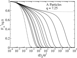
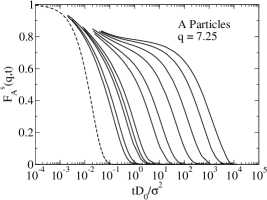
Figure 2: Incoherent intermediate scattering function for the A particles for $q=7.25$. (a) Predicted by the mode-coupling theory. (b) Calculated from the Brownian dynamics simulations. The scattering functions are shown for the same reduced temperatures $\epsilon=(T-T_{c})/T_{c}$. The reduced temperatures are 3.5977, 2.4483, 1.2989, 1.0690, 0.8391, 0.3793, 0.2644, 0.1494, 0.0805, 0.0345, 0.0115 listed from left to right. The dashed line in both figures correspond to the limit of non-interacting particles. The dotted line in figure (a) is the incoherent intermediate scattering function calculated at $T_{c}^{theory}$.

In Fig. 3a we compare the incoherent intermediate scattering functions for $\epsilon=3.5977$, 0.8391 0.0805, and 0.0115 for the A particles at $q=7.25$, and in Fig. 3b we show the comparison for the same reduced temperatures for the B particles at $q=5.75$. At the higher reduced temperatures there is very good agreement between the mode-coupling calculations and the Brownian dynamics simulations. For $0.0345<\epsilon<0.8391$ the characteristic decay time of the scattering functions calculated from the mode-coupling theory is less than that of the Brownian dynamics simulation. For reduced temperatures equal to and below 0.0345, the mode-coupling theory predicts a longer decay time for the self intermediate scattering functions for this value of $q$. However, the shape of the incoherent intermediate scattering functions are similar in the $\alpha$ relaxation region.

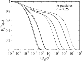
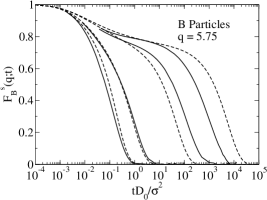
Figure 3: The incoherent intermediate scattering function for the A and B particles predicted by the mode-coupling theory (dashed lines) and calculated from the Brownian dynamics simulations (solid lines) for $\epsilon=3.598$, 0.839, 0.0805 and 0.0115 listed from left to right.

Kob, Nauroth, and Sciortino KobNauroth compared the self intermediate scattering functions obtained from Newtonian dynamics simulations and predicted by the mode-coupling theory. The input temperature in the mode-coupling theory was adjusted so that the relaxation time of $S_{AA}(q,t)/S_{AA}(q)$ was correctly reproduced for one wave vector around the first peak of $S_{AA}(q)$. The procedure followed by Kob et al. requires that the characteristic decay time is the same in the simulations and the mode-coupling theory calculations. Kob et al. observed that the shape of the scattering functions and its wave vector dependence is accurately described by the theory for reduced temperatures above 0.071. We discuss the wave vector dependence of the relaxation time in section VIII.

The mode-coupling theory predicts power law divergence of the characteristic decay time of the intermediate scattering functions. Specifically, we define the $\alpha$ relaxation time as the time when the incoherent intermediate scattering function decays to $e^{-1}$ of its initial value, $F_{\alpha}^{s}(q,\tau_{\alpha})=e^{-1}$. In Fig. (4) we show the $\alpha$ relaxation time for the A and B particles as a function of reduced temperature. We fit the $\alpha$ relaxation time to the function $a[(T-T_{c})/T_{c}]^{-\gamma}$. We fit the Brownian dynamics results to reduced temperatures from 0.8391 to 0.1495, which corresponds to the same reduced temperatures fit in an earlier work FlennerSzamel2 . We used this range of temperatures since this is the temperature range in which a power law fits the $\alpha$ relaxation time well for a transition temperature of 0.435. For the mode-coupling theory calculations, we fit the power law to reduced temperatures equal to and below 0.0345. The exponents in the power law fits are given in the figure.

The exponents from the mode-coupling calculations are close to but slightly larger than the exponents found from the simulations. Note that the exponent obtained from solving the mode-coupling equations for the single component hard sphere system Fuchs is the same as the exponents predicted by the mode coupling coupling theory for the binary Lennard-Jones system. The exponents determined from simulations are slightly different than the exponents reported in an earlier work FlennerSzamel2 , since we are fitting $\tau_{\alpha}D_{0}$ here and we fit $\tau_{\alpha}$ in the other work. We find, as other authors have also observed KobAndersen , that the exponents determined from the simulations are different for the A and the B particles. However, this difference is within the 3% uncertainty in the exponents. Note that the mode coupling theory predicts the same exponents for the A and B particles, and the same exponents for the $\alpha$ relaxation time and the self diffusion coefficient.

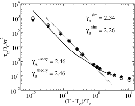
Figure 4: The $\alpha$ relaxation time calculated from the Brownian dynamics simulations (symbols) and predicted by the mode-coupling theory (solid and dashed lines) for the the A and B particles. The A particles are represented by the closed symbols and the solid line. The B particles are represented by the open symbols and the dashed line. The lines nearly overlap. The dotted lines are fits of the simulation data to the function $a[(T-T_{c})/T_{c}]^{-\gamma}$. The exponents to the power law fits are given in the figure along with the exponents to power law fits to the predictions of the mode-coupling theory.

Furthermore, the predictions of the mode-coupling theory follow the asymptotic power law behavior for reduced temperatures smaller than $\epsilon\approx 0.08$. This is in contrast with the results of simulations, which can only be fit to power laws in a restricted range $0.1495<\epsilon<0.8391$. On the other hand, it has been observed in experiments that the power law behavior of $\tau_{\alpha}$ is valid for reduced temperatures up to 0.5 Du .

VI Mean Square Displacement

To derive the mode-coupling theory predictions for the mean square displacement we use the small $q$ expansion of the incoherent intermediate scattering function Kaur ,

$$F_{\alpha}^{s}(q,t)=\sum_{n=0}^{\infty}(-1)^{n}\frac{q^{2n}}{(2n+1)!}\left<\delta r_{\alpha}^{2n}(t)\right>,$$ (20)

where $\left<\delta r_{\alpha}^{2n}(t)\right>=\left<|\vec{r}\,_{i}^{\alpha}(t)-\vec{r}\,_{i}^{\alpha}(0)|^{2n}\right>$. Inserting Eq. (20) into the equation for the incoherent intermediate scattering function, Eq. (13), and expanding $M_{\alpha}^{s}(q,t)$ in a Taylor series

$$M_{\alpha}^{s}(q,t)=\mathcal{M}_{\alpha}^{0}(t)+q^{2}\mathcal{M}_{\alpha}^{2}(t)+q^{4}\mathcal{M}_{\alpha}^{4}(t)+\dots$$ (21)

results in the equation of motion

$$\frac{\partial}{\partial t}\left<\delta r_{\alpha}^{2}(t)\right>=6D_{0}-\int_{0}^{t}\mbox{d}u\mathcal{M}_{\alpha}^{0}(t-u)\frac{\partial}{\partial u}\left<\delta r_{\alpha}^{2}(u)\right>$$ (22)

where

$$\mathcal{M}_{\alpha}^{0}(t) = \lim_{q\rightarrow 0}M_{\alpha}^{s}(q,t)$$ (23)

$$= \frac{D_{0}V}{6\pi^{2}N_{\alpha}}\int_{0}^{\infty}\mbox{d}k\>k^{4}\>F_{\alpha}^{s}(k,t)$$

$$\times\sum_{\delta\delta^{\prime}}C_{\alpha\delta}(k)S_{\delta\delta^{\prime}}(k,t)C_{\alpha\delta^{\prime}}(k).$$

This equation was solved using a variation of the procedure described in the appendix.

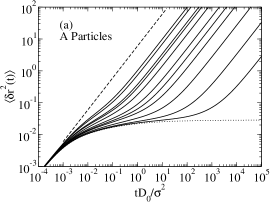
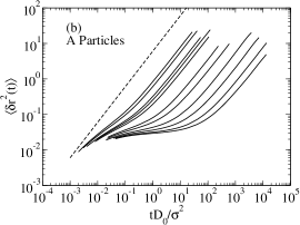
Figure 5: Mean square displacement for the A particles. (a) Predicted by the mode-coupling theory. (b) Calculated from the Brownian dynamics simulations. The solid lines correspond to the same reduced temperatures $\epsilon=(T-T_{c})/T_{c}$ in the mode-coupling theory calculations and the Brownian dynamics simulations. The reduced temperatures are 3.5977, 2.4483, 1.2989, 1.0690, 0.8391, 0.3793, 0.2644, 0.1494, 0.0805, 0.0345, 0.0115 listed from left to right. The dashed line corresponds to the limit of non-interacting particles and the dotted line in figure (a) is the mean square displacement calculated at $T_{c}^{theory}$.

We present the mode-coupling theory predictions and simulations results in Figs. 5a and 5b, respectively, for the A particles. The results for the B particles are similar. The solid lines correspond to the same reduced temperatures for the mode-coupling calculations and the Brownian dynamics simulations. The dotted line in Fig. 5a is the mean square displacement at $T_{c}^{theory}$. The dashed line in both figures corresponds to motion in the limit of non-interacting particles, i.e. a purely diffusive motion with a diffusion coefficient $D_{0}$. At all temperatures the short time motion is diffusive with a diffusion coefficient $D_{0}$. For the mode-coupling theory calculations, the short time diffusion coefficient is one, but the short time diffusion coefficient is temperature dependent in the Brownian dynamics simulations. Note, however, that the time axes are scaled to compensate for this difference.

The mode-coupling theory correctly predicts the existence of the plateau region in the log-log plot of the mean square displacement for temperature close to the transition temperature. The plateau represents a localization of the particles for several decades in time and is associated with the cage effect. According to the mode-coupling theory, above the transition temperature the long time motion is diffusive with a self diffusion coefficient $D>0$. Also, at and below the mode-coupling transition temperature, there is structural arrest and $D=0$.

In Fig. 6 we show the mean square displacements for reduced temperatures $\epsilon=3.5977$, 0.8391 0.0805, 0.0115 calculated using the mode-coupling theory (dashed lines) and obtained from the Brownian dynamics simulations (solid lines) for the A and B particles. The A particles are shown in the upper figure and the B particles are shown in the lower figure. The mean square displacement agrees reasonably well with the predictions of the mode-coupling theory for reduced temperatures equal to and above 0.0805 for both the A and B particles at all times. However, for reduced temperatures below $0.0805$, the mean square displacement is not accurately predicted by the mode-coupling theory.

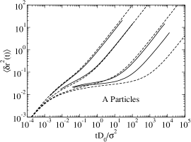
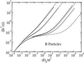
Figure 6: The mean square displacement for the A and B particles predicted by the mode-coupling theory (dashed lines) and calculated from the Brownian dynamics simulations (solid lines). The reduced temperatures are $\epsilon=3.5977$, 0.839, 0.0805 and 0.0115 listed from left to right.

For all reduced temperatures smaller than $\epsilon=0.8391$, there is an obvious plateau in the Brownian dynamics simulations and in the mode-coupling theory calculations. We define the height of the plateau region as the inflection point in the logarithm of the mean square displacement versus the logarithm of time. At small reduced temperatures the height of the plateau predicted by the theory agrees reasonably well with that obtained from simulations, Fig. 7. In particular, at $\epsilon=0.0115$, the plateau is predicted by the theory at a value of the mean square displacement of around 0.028 for the A particles and it occurs in the Brownian dynamics simulations at around 0.029. For the B particles at $\epsilon=0.0115$, the plateau is predicted by the theory to be around a value of 0.053 and it is around 0.043 in the simulations. However, the temperature dependence of the plateau according to the theory and in the simulations is very different. The theory predicts that the plateau height as a function of reduced temperature is essentially constant until around $\epsilon=0.8391$, and the plateau height increases slightly with increasing temperature. The plateau height calculated from the simulations increases with temperature faster than predicted by the theory. For reduced temperatures above 0.3793, it is difficult to calculate the inflection point for the Brownian dynamics simulations accurately. Note that in the temperature range in which the theory gives reasonably accurate predictions for the incoherent scattering function and the mean square displacement, the plateau height resulting from the theory is quite a bit smaller than that obtained from simulations. For example, for $\epsilon=0.3793$ the mean square displacement at the inflection point predicted by the theory is around 0.024 and 0.053 for the A and B particles, respectively, whereas in simulations it occurs around 0.040 and 0.12 for the A and B particles, respectively.

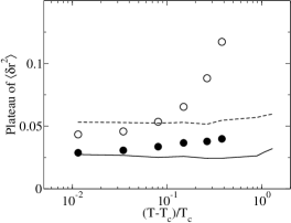
Figure 7: Comparison of the plateau value of the mean square displacement versus temperature. The symbols are the simulation results and the lines are the predictions of the mode-coupling theory. The A particles are represented by the closed symbols and the solid line, and the B particles are represented by the open symbols and the dashed line.

We obtain the self diffusion coefficient $D$ from the slope of the mean square displacement at long times, i.e. from $D=\lim_{t\rightarrow\infty}\left<\delta r_{\alpha}^{2}(t)\right>/(6t)$. Within the mode-coupling theory, we can also calculate $D$ from the equation

$$\frac{D}{D_{0}}=\frac{1}{1+\int_{0}^{\infty}\mbox{d}t\mathcal{M}_{\alpha}^{0}(t)}.$$ (24)

Both procedures agree to within one percent. The diffusion coefficients predicted by the theory and obtained from Brownian dynamics simulations are shown in Fig. 8 as a function of reduced temperature. The mode-coupling theory provides a good prediction for the diffusion coefficients for $\epsilon\geq 0.0805$, but the diffusion coefficients predicted by the theory are slightly larger than the ones found from simulations. At lower reduced temperatures the theory strongly underestimates the diffusion coefficients. In addition, the theory does not capture the increasing difference between the diffusion coefficients of the A and the B particles.

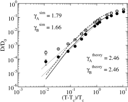
Figure 8: The diffusion coefficient determined from the Brownian dynamics simulation (symbols) and the mode-coupling theory (solid and dashed lines). The closed symbols and the solid line are the results for the A particles. The open symbols and the dashed line are the results for the B particles. The dotted line is a fit of the simulation data to the function $a[(T-T_{c})/T_{c}]^{\gamma}$. The exponents to the power law fits are given in the figure along with the exponents to power law fits to the predictions of the mode-coupling theory.

We fit $D/D_{0}$ to power laws of the form $a[(T-T_{c})/T_{c}]^{\gamma}$; the exponents are given in Fig. 8. For the mode-coupling theory fit we use reduced temperatures less than 0.0345 whereas for the Brownian dynamics simulations we fit the range $0.1495\leq\epsilon\leq 0.8391$. The exponents for the Brownian dynamics simulations are slightly different than what has been reported in an earlier work FlennerSzamel2 , since we are fitting $D/D_{0}$ here and $D$ there. The exponents predicted by the mode-coupling theory are considerably larger than those obtained from the fits to simulations’ results. Note that the exponents for the diffusion coefficient calculated from the theory is the same as the exponents found for the $\alpha$ relaxation time. Moreover, the exponents found from the mode-coupling calculations are the same for the A and the B particles.

The reduced temperatures in which it is possible to fit the mode-coupling results well with a power law is similar to what was found for the $\alpha$ relaxation time, i.e. that the power law provides a good fit up to a reduced temperature of around 0.08.

We would like to point out that power laws fit the predictions of the mode-coupling theory reasonably well for the same reduced temperatures in which we fit power laws to the results of the Brownian dynamics simulations. If we fit the predictions of the mode-coupling theory to power laws using the range $0.1495\leq\epsilon\leq 0.8391$, the resulting exponents are different from the true exponents (i.e. from the exponents describing the the true asymptotic power law behavior) but they differ by at most 12% from the exponents obtained from the Brownian dynamics simulations. This should be compared with the 48% difference between the true mode-coupling theory exponent and the exponent for the B particles obtained from the Brownian dynamics simulations using the range $0.1495\leq\epsilon\leq 0.8391$.

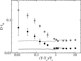
Figure 9: Product of the diffusion coefficient and the $\alpha$ relaxation time determined from the Brownian dynamics simulation (symbols) and the mode-coupling theory (solid and dashed lines). The closed symbols and the solid line are the results for the A particles. The open symbols and the dashed line are the results for the B particles. Note that for clarity we omitted the error bars for the lowest temperature point ($\epsilon=0.0115$) for the A particles; at the lowest temperature for the A particles $D\tau_{\alpha}=0.0585\pm 0.054$

Finally, in Fig. 9 we compare the temperature dependence of the product of the diffusion coefficient and the $\alpha$ relaxation time predicted by the mode-coupling theory and obtained from simulations. In the high temperature regime one usually expects that the Stokes-Einstein relation is valid and $D\tau_{\alpha}$ is temperature-independent. The decoupling of the diffusion and structural relaxation has been identified as one of the signatures of increasingly heterogeneous dynamics MEreview . The mode-coupling theory predicts an essentially temperature-independent $D\tau_{\alpha}$. In contrast, simulations show that the product of the diffusion coefficient and the $\alpha$ relaxation time starts increasing with temperature below approximately $\epsilon=1$. Note that this value of the reduced temperature corresponds to a temperature that is close to the so-called onset temperature identified for the Kob-Andersen model by Brumer and Reichman onset .

VII Non-Gaussian Parameter

At short and long times, the motion of the particles is Fickian and the self part of the van Hove correlation function is Gaussian. For intermediate times, the van Hove correlation function deviates from Gaussian. To examine the non-Gaussian nature of the van Hove correlation function, we calculated the non-Gaussian parameter

$$\alpha_{2}(t)=\frac{3}{5}\frac{\left<\delta r^{4}_{\alpha}(t)\right>}{\left<\delta r^{2}_{\alpha}(t)\right>^{2}}-1.$$ (25)

For the calculation of $\alpha_{2}(t)$, we first calculated the mean square displacement (see section VI) and then we calculated $\left<\delta r^{4}_{\alpha}(t)\right>$. The equation of motion for $\left<\delta r^{4}_{\alpha}(t)\right>$ is derived using the same method as the equation for $\left<\delta r^{2}_{\alpha}(t)\right>$. The resulting equation of motion is

$$\frac{\partial}{\partial t}\left<\delta r^{4}_{\alpha}(t)\right> = 20D_{0}\left<\delta r^{2}_{\alpha}(t)\right>$$

$$-\int_{0}^{t}\mbox{d}u\mathcal{M}_{\alpha}^{0}(t-u)\frac{\partial}{\partial u}\left<\delta r^{4}_{\alpha}(u)\right>$$

$$+10\int_{0}^{t}\mbox{d}u\mathcal{M}_{\alpha}^{2}(t-u)\frac{\partial}{\partial u}\left<\delta r^{2}_{\alpha}(u)\right>$$

where

$$\mathcal{M}_{\alpha}^{2}(t) = \frac{VD_{0}^{2}}{10\pi^{2}N_{\alpha}}$$ (27)

$$\times\int\mbox{d}k\ k^{4}\left[\frac{2}{3k}\frac{\partial}{\partial k}F_{\alpha}^{s}(k,t)+\frac{\partial^{2}}{\partial k^{2}}F_{\alpha}^{s}(k,t)\right]$$

$$\times\sum_{\delta\delta^{\prime}}C_{\alpha\delta}(k)S_{\delta\delta^{\prime}}(k,t)C_{\alpha\delta^{\prime}}(k).$$

In principle, it is also possible to calculate the non-Gaussian parameter by fitting $F_{\alpha}^{s}(q,t)$ in the small wave vector limit Kaur . We found that this procedure was difficult to follow using the structure factors calculated from simulations, and small numerical uncertainties in the small $q$ values of $F_{\alpha}^{s}$ can result in large changes in the non-Gaussian parameter. For short times, the integrals involving memory functions in Eqs. (22) and (LABEL:r4eq) are close to zero. Thus, for short times $\left<\delta r^{2}(t)\right>\approx 6D_{0}t$ and $\left<\delta r^{4}(t)\right>\approx 60D_{0}^{2}t^{2}$, therefore $\alpha_{2}(t)\approx 0$. At long times, the motion is once again Fickian, the self part of the van Hove correlation function is Gaussian and $\alpha_{2}(t)=0$. In our calculations, $\alpha_{2}(t)$ does not go to zero at long times, but rather to a value around $5\times 10^{-3}$. We believe that this result can be attributed to numerical errors; it does not imply that $\alpha_{2}(t)$ is nonzero for $t\rightarrow\infty$.

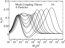
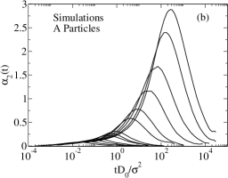
Figure 10: The non-Gaussian parameter for the A particles. (a) Predicted by the mode-coupling theory. (b) Calculated using the Brownian dynamics simulations. The reduced temperatures $\epsilon=(T-T_{c})/T_{c}$ are 3.5977, 2.4483, 1.2989, 1.0690, 0.8391, 0.3793, 0.2644, 0.1494, 0.0805, 0.0345, 0.0115. In figure (a), there is one peak for $\epsilon=3.5977$, and a wider single peak for 2.4483 (dashed lines). For all the other reduced temperatures there are two peaks, and the larger peak position of the second peak corresponds to a lower reduced temperature. In figure (b), the larger peak heights correspond to lower reduced temperatures.

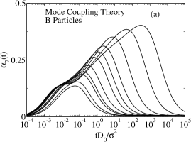
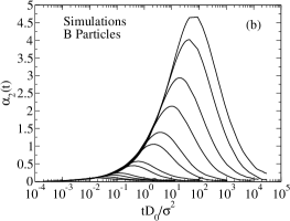
Figure 11: The non-Gaussian parameter for the B particles. (a) Predicted by the mode-coupling theory. (b) Calculated from the Brownian dynamics simulations. The reduced temperatures $\epsilon=(T-T_{c})/T_{c}$ are 3.5977, 2.4483, 1.2989, 1.0690, 0.8391, 0.3793, 0.2644, 0.1494, 0.0805, 0.0345, 0.0115 where the lower reduced temperatures correspond to larger peak heights.

We show the non-Gaussian parameters for the A particles in Fig. 10. The upper panel shows the predictions of the mode-coupling theory and the lower panel shows the results of the Brownian dynamics simulations. According to the mode-coupling calculations, there is one peak at high reduced temperatures, but for $\epsilon\leq 1.2989$ there are two peaks. Two peaks have been observed before in mode-coupling calculations of $\alpha_{2}(t)$ for other systems Kaur . The first peak is around the beginning of the plateau region of the mean square displacement and the initial decay of the scattering functions. The position of the first peak decreases for decreasing temperature, but is almost constant for $\epsilon\leq 0.8391$. The second peak is around the $\alpha$ relaxation time which corresponds to just after the plateau region of the mean square displacement. The position of the second peak increases with decreasing temperature and roughly follows the temperature dependence of the $\alpha$ relaxation time, Fig. 12a.

There is only one peak in $\alpha_{2}(t)$ according to the Brownian dynamics simulations, Fig. 10b. The position of this peak is greater than the $\alpha$ relaxation time at higher temperatures, but it increases slower with decreasing temperature than the $\alpha$ relaxation time starting at around $\epsilon=0.8391$.

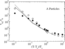
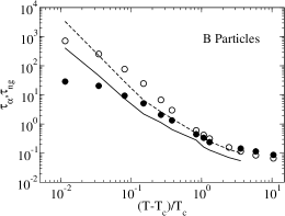
Figure 12: The peak position of the non-Gaussian parameter compared to the $\alpha$ relaxation time. The symbols are the simulation results and the lines are the predictions of the mode-coupling theory. The open symbols and dashed lines are the $\alpha$ relaxation time. The closed symbols and the solid lines are the peak positions of the non-Gaussian parameter.

The mode coupling theory predicts one peak at all temperature for the B particles. However, there is a prominent shoulder for $\epsilon\leq 1.2989$, the same reduced temperatures in which there are two peaks in the non-Gaussian parameter for the A particles. The position of the shoulder follows the same temperature dependence as the position of the first peak in the non-Gaussian parameter for the A particles. The peak position in $\alpha_{2}(t)$ predicted by the mode-coupling theory is less than the $\alpha$ relaxation time at all temperatures, and it increases with decreasing temperature at close to the same rate as the $\alpha$ relaxation time, Fig. 12b.

The non-Gaussian parameter for the B particles obtained from the Brownian dynamics simulation is shown in Fig. 11b. There is only one peak for all temperatures. The position of the peak is greater than the $\alpha$ relaxation time for higher temperatures, but the position increases slower with decreasing temperature than the $\alpha$ relaxation time and is much less than the $\alpha$ relaxation time at small reduced temperatures, Fig. 12b.

To summarize, the time dependence of the non-Gaussian parameter calculated using the mode-coupling theory is significantly different from what is obtained from the Brownian dynamics simulations. More importantly, the mode-coupling theory strongly underestimates the deviations from Gaussian (i.e. Fickian) diffusive motion: the heights of non-Gaussian parameters predicted by the theory are almost an order of magnitude smaller than those obtained from the Brownian dynamics simulations. We show in the next section that the simulations show even stronger non-Gaussian effects on somewhat longer time scales.

VIII Probability distributions of the logarithm of single particle displacements

In an earlier work FlennerSzamel2 , we showed that as the temperature $T_{c}^{sim}=0.435$ is approached, the motion of the particles changes from a high temperature diffusive-like behavior to a low temperature hopping-like motion. To this end, we investigated probability distributions of the logarithm of single particle displacements Reichman ; Puertas . The probability distribution of the logarithm of single particle displacements at a time t, $P\bm{(}\log_{10}(\delta r);t\bm{)}$, can be obtained from the self van Hove correlation function, $G_{s}(\delta r,t)=\left<\delta\left(|\vec{r}\,_{i}^{\alpha}(t)-\vec{r}\,_{i}^{\alpha}(0)|-\delta r\right)\right>$, by the following transformation $P\bm{(}\log_{10}(\delta r);t\bm{)}=\ln(10)4\pi\delta r^{3}G_{s}(\delta r,t)$. Note that if the motion of a tagged particle is diffusive at all times with a diffusion coefficient $D$, then the self van Hove correlation function $G_{s}(\delta r,t)=(1/(4\pi Dt)^{\frac{3}{2}})\exp(-\delta r^{2}/4Dt)$ and it can be shown that the shape of the probability distribution $P\bm{(}\log_{10}(\delta r);t\bm{)}$ is time-independent. In particular, the peak height of $P\bm{(}\log_{10}(\delta r);t\bm{)}$ does not depend time and is equal to $\ln(10)\sqrt{54/\pi}\ e^{-3/2}\approx 2.13$. Thus, deviations from this height represent deviations from Gaussian behavior of $G_{s}(\delta r,t)$.

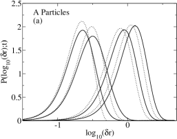
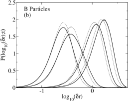
Figure 13: The probability distribution of the logarithm of single particle displacements predicted by the mode-coupling theory (dotted lines) compared to the probability distributions calculated from the Brownian dynamics simulations (solid lines) for $\epsilon=0.8391$. (a) A particles. (b) B particles. The times shown are 0.25, 1.0, 10, and 20 times the $\alpha$ relaxation time; note that we use the A-particles and the B-particles $\alpha$ relaxation time in (a) and (b), respectively.

We show a comparison of $P\bm{(}\log_{10}(\delta r);t\bm{)}$ in Fig. 13 for the A and B particles calculated from the simulations (solid lines) and from the mode-coupling theory (dotted lines) for the reduced temperature $\epsilon=0.8391$ for several different times: 0.25, 1.0, 5.0, and 10.0 $\tau_{\alpha}$. It should be noted that in Figs. 13 and 14 we use the A and the B particles $\alpha$ relaxation times in panels (a) and (b), respectively; moreover, we use the $\alpha$ relaxation times obtained from simulations for the simulation results and the $\alpha$ relaxation times predicted by the mode-coupling theory for the theoretical results. At this temperature the mode-coupling theory describes the probability distributions reasonably well.

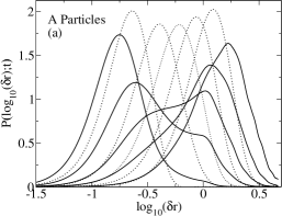
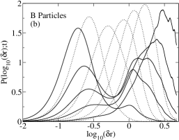
Figure 14: The probability distribution of the logarithm of single particle displacements predicted by the mode-coupling theory (dotted lines) compared to the probability distributions calculated from the Brownian dynamics simulations (solid lines) for $\epsilon=0.0115$. (a) A particles. (b) B particles. The times shown are 0.1, 1, 2.5, 5, and 10 times the $\alpha$ relaxation time; note that we use the A-particles and the B-particles $\alpha$ relaxation time in (a) and (b), respectively.

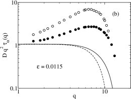
Figure 15: The product $Dq^{2}\tau_{\alpha}(q)$ for $\epsilon=0.8391$ and 0.0115. The symbols are the results of the Brownian dynamics simulations and the lines are the predictions of the mode-coupling theory. The A particles are represented by the closed symbols and the solid lines, and the B particles are represented by the open symbols and the dashed lines.

In Fig. 14 we show a comparison of $P\bm{(}\log_{10}(\delta r);t\bm{)}$ for the A and B particles calculated from the simulations (solid lines) and from the mode-coupling theory (dotted lines) for several different times at a reduced temperature of $\epsilon=0.0115$ (recall that, as in Fig. 13, we use the A and the B particles $\alpha$ relaxation times in panels (a) and (b), respectively; moreover we use the $\alpha$ relaxation times obtained from simulations for the simulation results and the $\alpha$ relaxation times predicted by the mode-coupling theory for the theoretical results). This is the lowest reduced temperature in which we can directly compare the predictions of the mode-coupling theory to the simulation results. There is a dramatic difference in the shape of the curves over the time interval shown in the figure. At intermediate times bimodal distributions are obtained from Brownian dynamics simulations whereas the mode-coupling theory predicts unimodal distributions at all times. The bimodal distributions suggests that a portion of the particles are undergoing hopping-like motion with a large distribution of hopping rates. This hopping-like motion is not predicted by the mode-coupling theory.

In an earlier work FlennerSzamel2 , we observed in the simulations that the time in which both peaks are about equal height is longer than the time indicated by the peak position of the non-Gaussian parameter $\alpha_{2}(t)$. We defined a new parameter $\gamma(t)=\frac{1}{3}\left<\delta r^{2}\right>\left<1/\delta r^{2}\right>-1$ whose peak position occurs at the same time as when the two peaks in $P\bm{(}\log_{10}(\delta r);t\bm{)}$ are approximately the same height for temperatures in which there are two peaks. It was found that the peak position of $\gamma(t)$ has the same temperature dependence as the $\alpha$ relaxation time.

At temperatures in which we see evidence of the hopping-like motion when we examine the probability distribution $P\bm{(}\log_{10}(\delta r);t\bm{)}$, the wave vector dependent $\alpha$ relaxation time is qualitatively different in the simulation than predicted by mode-coupling theory.

In Fig. 15 we show $Dq^{2}\tau_{\alpha}(q)$, where $\tau_{\alpha}(q)$ is the wave vector dependent $\alpha$ relaxation time defined as the time when $F_{\alpha}^{s}\bm{(}q,\tau_{\alpha}(q)\bm{)}=e^{-1}$. The lines are the predictions of the mode-coupling theory and the circles are the results of the Brownian dynamics simulations. For small wave vectors, the product $Dq^{2}\tau_{\alpha}(q)$ is one. For the reduced temperature of $\epsilon=0.8391$, Fig. 15a, $\tau_{\alpha}(q)^{-1}=Dq^{2}$ until $q\approx 5$. At larger wave vectors there is a crossover from the small wave vector relationship to the large wave vector limit $\tau_{\alpha}(q)^{-1}=D_{0}q^{2}$ (this large wave vector limit follows from the fact that memory functions vanish in the large wave vector limit).

In contrast, for lower reduced temperatures, there is a qualitative difference between the wave vector dependent $\alpha$ relaxation time predicted by the theory and calculated from the Brownian dynamics simulations. In Fig. 15b we show the product $Dq^{2}\tau_{\alpha}(q)$ for the reduced temperature $\epsilon=0.0115$. At small wave vectors the simulation results approach the asymptotic behavior $\tau_{\alpha}(q)^{-1}=Dq^{2}$. At intermediate wave vectors, $1.5\leq q\leq 7.5$, the values of $Dq^{2}\tau_{\alpha}(q)$ calculated from the simulation increase with a peak somewhere between $6.5<q<7.5$. At large wave vectors, the $\alpha$ relaxation time reaches its limiting behavior $\tau_{\alpha}(q)^{-1}=D_{0}q^{2}$. On the other hand, the mode coupling theory predicts a monotonically decaying $Dq^{2}\tau_{\alpha}(q)$ with essentially the same behavior at low and high reduced temperatures, Fig.15.

We should point out that the increase of $Dq^{2}\tau_{\alpha}(q)$ with wave vector for intermediate wave vectors was previously found in the Kob-Andersen system by Berthier Berthier . Also, the increase of $Dq^{2}\tau_{\alpha}(q)$ has been predicted within the theoretical approach of Schweizer and Saltzman Ken . Finally, Berthier, Chandler and Garrahan found a similar behavior in one-dimensional facilitated kinetic Ising models BCG . Here we emphasize that this behavior correlates with strong deviations from Fickian diffusion visible in the probability distribution $P\bm{(}\log_{10}(\delta r);t\bm{)}$.

IX Conclusions

We have conducted an extensive comparison of the predictions of the mode-coupling theory to Brownian dynamics simulations. As has been previously observed, qualitatively, predictions of the mode-coupling theory agree well with simulations. Namely, the mode-coupling theory accurately predicts the two step relaxation observed in the scattering functions, the existence of the plateau region observed in the mean square displacement, and the power law behavior of the self diffusion coefficient and the $\alpha$ relaxation time.

The mode-coupling theory overestimates the feedback mechanism in the memory functions, resulting in a transition temperature $T_{c}^{theory}=0.9515$ much greater than the temperature $T_{c}^{sim}=0.435$ inferred from simulations. The transition temperature found in simulations is determined by fitting the diffusion coefficient and the $\alpha$ relaxation time to power laws. It should be noted that this temperature is sensitive to the range of temperatures used in the power law fits FlennerSzamel2 . While the transition temperatures are vastly different, we find that the mode-coupling theory gives good quantitative results of many time dependent quantities if they are compared at the same reduced temperature $\epsilon=(T-T_{c})/T_{c}$.

The self intermediate scattering functions and the mean square displacement resulting from simulations are well described by the mode-coupling theory for reduced temperatures greater than 0.08. For temperatures close to $T_{c}$ the mode-coupling theory predicts divergence of the self intermediate scattering function’s relaxation time and vanishing of the self diffusion coefficient. There is no divergence of the relaxation time or vanishing of the self diffusion coefficient in the Brownian dynamics simulations.

The non-Gaussian parameter calculated from the simulations are quite different than the non-Gaussian parameter predicted by the mode-coupling theory. The mode-coupling theory predicts two peaks in $\alpha_{2}(t)$ for reduced temperatures $\epsilon\leq 1.2989$ for the A particles, and a shoulder at short times and a peak at longer times for the B particles. There is only one peak in the non-Gaussian parameter calculated from the simulation for all temperatures for both the A and B particles. Furthermore, the position of the second peak for the A particles and the only peak for the B particles predicted by the mode-coupling theory has a different temperature dependence than the position of the peak observed in the Brownian dynamics simulations. The mode-coupling theory predicts that the position of the second peak roughly follows the $\alpha$ relaxation time close to $T_{c}$, while the position of the peak for the Brownian dynamics simulations increases slower with decreasing temperature than the $\alpha$ relaxation time. Finally, the theory underestimates the height of the non-Gaussian parameter peak by almost an order of magnitude.

We calculated the probability of the logarithm of single particle displacements $P\bm{(}\log_{10}(\delta r);t\bm{)}$ which is sensitive to hopping-like motion. At high reduced temperatures, there is no hopping-like motion evident in the Brownian dynamics simulations and $P\bm{(}\log_{10}(\delta r);t\bm{)}$ is accurately described by the mode-coupling theory. For low reduced temperatures, there is little agreement between the mode-coupling theory and the simulations. At the lowest reduced temperature studied in this work, $\epsilon=0.0115$, the hopping-like motion is very evident in the Brownian dynamics simulations, but is not predicted by the mode-coupling theory. We believe that this hopping-like motion is responsible for the absence of the divergence of the relaxation time or vanishing of the self diffusion coefficient in the simulations.

For low reduced temperatures, the mode-coupling theory does not predict the proper wave vector dependence of the $\alpha$ relaxation time. The theory predicts that at all temperatures the product $Dq^{2}\tau(q)$ is one for small wave vectors and it decreases monotonically with increasing wave vector. In contrast, at low temperatures Brownian dynamics simulations show a peak in the product $Dq^{2}\tau(q)$.

To summarize, we found that close but not too close to the transition temperature the mode-coupling theory does predict most time-dependent quantities reasonably well. At very small reduced temperatures there is a hopping-like motion present in the simulations which is not accounted for by the standard version of the mode-coupling theory. Signatures of the hopping-like motion include the two-peak structure of the probability of the logarithm of particle displacements and non-trivial wave vector dependence of the $\alpha$ relaxation time.

Appendix A Numerical Routines

In this section we will outline the numerical routines that were used to solve many of the equations given in this paper. Since the time dependent quantities were solved over many decades in time, it is not possible to solve these equations using normal Gaussian quadrature, and special algorithms must be implemented. While these techniques have been outlined in the literature previously FuchsMCT ; Miyazaki , they have not been described in detail. In this appendix we will describe numerical routines used to calculate integrals of the form

$$\int\mbox{d}\vec{k}\ F(|\vec{q}-\vec{k}|)G(k)$$ (28)

when F(k) and G(k) are only known on a grid of equally spaced wave vectors and and how to solve equations of the form

$$\dot{F}_{q}(t)=aF_{q}(t)+\int_{0}^{t}\mbox{d}u\ M_{q}(F_{q},t-u)\dot{F}_{q}(u)$$ (29)

for many decades in time. The dot denotes a derivative with respect to time. It is important to note that the function $M_{q}$ not only depends on time $t$, but also on the functions $F_{q}(t)$.

The integrals of the memory function in the mode-coupling theory are all of the form given by Eq. 28. To calculate the integral, the functions are generally only known on a grid of equally spaced wave vectors. Furthermore the calculation of these integrals are the most computationally expensive part of the program, and extrapolation between grid points can increase the calculation time significantly. The first step is to introduce the change of variables $\vec{p}=\vec{k}-\vec{q}/2$, then convert to spherical polar coordinates. This allows integration over one angular variable and the integral becomes

$$2\pi\int p^{2}\sin\phi\ \mbox{d}p\ \mbox{d}\phi\ F\left(\left|\vec{p}-\frac{\vec{q}}{2}\right|\right)G\left(\left|\vec{p}+\frac{\vec{q}}{2}\right|\right).$$ (30)

Then make another change of variables to

$$x = \left|\vec{p}+\frac{\vec{q}}{2}\right|=\sqrt{p^{2}+q^{2}/4+pq\cos\phi}$$ (31)

$$y = \left|\vec{p}-\frac{\vec{q}}{2}\right|=\sqrt{p^{2}+q^{2}/4-pq\cos\phi}$$ (32)

which results in the integral

$$\frac{2\pi}{q}\int_{0}^{\infty}x\mbox{d}x\int_{\left|x-q\right|}^{x+q}y\mbox{d}yF(y)G(x)$$ (33)

which can easily be calculated numerically using any number of quadrature techniques. There is one technical issue in using Eq. 33. As $q\rightarrow 0$ the integral over $y$ goes to zero, but the integral itself does not go to zero, see e.g. equation 23. While the effect is negligible for larger wave vectors, for small $q$ it is better to expand Eq. 28 in a Taylor series around $q=0$. We found that this had to be done to obtain accurate small $q$ values of varies quantities, e.g. the non-ergodicity parameter. In this work the Taylor series approximation was always used to calculate the integrals of the memory functions for the two smallest wave vectors.

Most of the equations solved in this paper has the form given by Eq. 29 and they must be solved for many decades in time. The basic algorithm is as follows. First an arbitrary time interval $\Delta t$ is broken into $4N$ equal segments of size $\delta t=\Delta t/4N$. It is assumed that the value of $F_{q}(t)$ for the first $2N$ segments is known. For each future time an equation of the form

$$F_{q}(t)=aH(F_{q},t)+b.$$ (34)

is solved. When $F_{q}(t_{i})$ has been calculated for all $4N$ times the time interval $\Delta t^{\prime}=2\Delta t$ is doubled. The new time integral in divided into $4N$ equal segments of size $\delta t^{\prime}=2\delta t$. Since $F(t)$ has been calculated up to $\Delta t^{\prime}/2$, a mapping of $\{F_{q}(t_{i})\}\rightarrow\{F_{q}(t_{j})\}$ can be defined where $t_{i}=i\delta t$ and $t_{j}=j\delta t^{\prime}$ and thus we know $F_{q}(t)$ for the first $2N$ segments of the new time interval, and the procedure is repeated.

First we will describe how to convert Eq. 29 into an equation of the form 34. Break the integral in Eq. 29 into two integrals, then integrate the integral starting at $t=0$ by parts to get

$$\int_{0}^{t}\mbox{d}u\ M_{q}(t-u)\dot{F}_{q}(u) = M_{q}(t-t_{2})F_{q}(t_{2})-M_{q}(t)F_{q}(0)$$ (35)

$$-\int_{0}^{t_{2}}\mbox{d}u\dot{M}_{q}(t-u)F_{q}(u)$$

$$+\int_{t_{2}}^{t}\mbox{d}uM_{q}(t-u)\dot{F}_{q}(u)$$

Next make a change of variables in the second integral in Eq. 35 to $\tau=t-u$ and break both integrals in Eq. 35 into integrals of length $\Delta t/2$. This results in the following exact form of the integral in Eq. 35,

$$M_{q}(t-t_{2})F_{q}(t_{2}) - M_{q}(t)F_{q}(0)$$

$$- \sum_{j=1}^{n_{1}}\int_{t_{j-1}}^{t_{j}}\mbox{d}u\dot{M}_{q}(t-u)F_{q}(u)$$

$$- \sum_{j=1}^{n2}\int_{t_{j-1}}^{t_{j}}\mbox{d}uM_{q}(u)\dot{F}_{q}(t-u).$$

Use the approximation that

$$\int_{t_{j-1}}^{t_{j}}\mbox{d}u\dot{A}(u)B(u) \approx \{A(t_{j})-A(t_{j-1})\}\frac{1}{\delta t}\int_{t_{j-1}}^{t_{j}}\mbox{d}uB(u)$$ (37)

$$\approx \{A(t_{j})-A(t_{j-1})\}\mathcal{I}\left[B(t_{j})\right]$$

where $\mathcal{I}\left[B(t_{j})\right]=(1/2)[B(t_{j-1})+B(t_{j})]$. We approximate $\dot{F}_{q}(t_{i})$ by

$$\dot{F}_{q}(t)\approx\frac{1}{2\delta t}F_{q}(t_{i-2})-\frac{2}{\delta t}F_{q}(t_{i-1})+\frac{3}{2\delta t}F_{q}(t_{i}),$$ (38)

but other approximations for the derivative can be used. Put all this together to get the equation

$$C_{1}F_{q}(t_{i})=C_{2}M_{q}(t_{i})+C_{3}$$ (39)

where

$$C_{1} = \frac{3}{2\delta t}-\mathcal{I}\left[M_{q}(t_{1})\right]-a$$

$$C_{2} = \mathcal{I}\left[F_{q}(t_{1})\right]-F_{q}(0)$$

$$C_{3} = \frac{2}{\delta t}F_{q}(t_{i-1})-\frac{1}{2\delta t}F_{q}(t_{i-1})$$

$$+M_{q}(t_{i-i2})F_{q}(t_{i2})-M_{q}(t_{i-1})$$

$$-F_{q}(t_{i-1})\mathcal{I}\left[M_{q}(t_{i2})\right]$$

$$-\sum_{j=2}^{i2}\left\{M_{q}(t_{i-j})-M_{q}(t_{i-j+1})\right\}\mathcal{I}\left[F_{q}(t_{j})\right]$$

$$-\sum_{j=2}^{i-i2}\left\{F_{q}(t_{i-j})-F_{q}(t_{i-j+1})\right\}\mathcal{I}\left[M_{q}(t_{j})\right]$$

which can be easily recast into the form of Eq. 34. Recall that $M_{q}(t_{i})$ depends on $F_{q}(t_{i})$. Equation 34 can be solved using any number of techniques used to find a fixed point of a set of equations. There is one equation of the form 34 for every $q$ vector, and $M_{q}(t_{i})$ depends on each $F_{q}(t_{i})$.

It remains to describe the mapping from $\Delta t$ to $\Delta t^{\prime}=2\Delta t$. For $1\leq j\leq 2N$,

$$F_{q}(t_{2i}) \rightarrow F_{q}(t_{j})$$ (41)

$$M_{q}(t_{2i}) \rightarrow M_{q}(t_{j}).$$ (42)

For $1\leq j\leq N$,

$$0.5\left\{\mathcal{I}\left[F_{q}(t_{2i})\right]+\mathcal{I}\left[F_{q}(t_{2i-1})\right]\right\} \rightarrow \mathcal{I}\left[F_{q}(t_{j})\right]$$

$$0.5\left\{\mathcal{I}\left[M_{q}(t_{2i})\right]+\mathcal{I}\left[M_{q}(t_{2i-1})\right]\right\} \rightarrow \mathcal{I}\left[M_{q}(t_{j})\right]$$

For $N+1\leq j\leq 2N$

$$\frac{1}{6}\left\{F_{q}(t_{2i})+4F_{q}(t_{2i-1})+F_{q}(t_{2i-2})\right\} \rightarrow \mathcal{I}\left[F_{q}(t_{j})\right]$$

$$\frac{1}{6}\left\{M_{q}(t_{2i})+4M_{q}(t_{2i-1})+M_{q}(t_{2i-2})\right\} \rightarrow \mathcal{I}\left[M_{q}(t_{j})\right].$$

Now there are values for $F,M,\mathcal{I}[F],\mathcal{I}[M]$ from $0\leq t\leq\Delta t^{\prime}/2$ and they can be calculated for $\Delta t^{\prime}/2<t\leq\Delta t^{\prime}$.

References

- (1) W. Götze, in Liquids, Freezing and Glass Transition, J.P. Hansen, D. Levesque, and J. Zinn-Justin, eds. (North-Holland, Amsterdam, 1991)).
- (2) S. P. Das, Rev. Mod. Phys. 76, 785 (2004).
- (3) P. Lunkenheimer, A. Pimenov and A. Loidl, Phys. Rev. Lett. 78, 2995 (1997).
- (4) J.L. Barrat, W. Götze and A. Latz, J. Phys.:Condens. Matter 1, 7163 (1989).
- (5) W. Kob and H.C. Andersen, Phys. Rev. Lett. 73, 1376 91994); Phys. Rev. E 51, 4626 (1995); Phys. Rev. E 52, 4134 (1995).
- (6) T. Franosch, M. Fuchs, W. Götze, M. R. Mayr, and A. P. Singh, Phys. Rev. E 55, 7153 (1997).
- (7) M. Fuchs, W. Götze and M.R. Mayr, Phys. Rev. E 58, 3384 (1998).
- (8) M. Nauroth and W. Kob, Phys. Rev. E 55, 657 (1997).
- (9) W. Kob, M. Nauroth and F. Sciortino, J. Non-Cryst. Solids 307-310, 181 (2002).
- (10) G. Foffi, W. Götze, F. Sciortino, P. Tartaglia, and Th. Voigtmann, Phys. Rev. E 69, 011505 (2004).
- (11) Th. Voigtmann, A.M. Puertas and M. Fuchs, Phys. Rev. E 70, 061506 (2004).
- (12) The alternative used in other stochastic dynamics simulations is to explicitly modify the noise in such a way that the center of mass does not move (W. Kob, private communication).
- (13) G. Nägele, Phys. Rep. 272, 215 (1996).
- (14) G. Nägele, J. Bergenholtz and J.K.G. Dhont, J. Chem. Phys. 110, 7037 (1999); G. Nägele and J.K.G. Dhont, J. Chem. Phys. 108, 9566 (1998).
- (15) M. Fuchs, W. Götze, I. Hofacker, and A. Latz, J. Phys.: Condens. Mat. 3, 5047 (1991).
- (16) K. Miyazaki, B, Bagchi and Yethiraj, cond-mat/0405326v1. Note that the published version of this manuscript (J. Chem. Phys. 121, 8120 (2004)) does not contain the detailed description of the numerical algorithm.
- (17) J.L. Barrat and A. Latz, J. Phys.: Condens. Mat. 2, 4289 (1990).
- (18) G. Szamel and E. Flenner, Europhys. Lett. 67, 779 (2004).
- (19) E. Flenner and G. Szamel, submitted to Phys. Rev. E; cond-mat/0505173.
- (20) W.M. Du, G. Li, H.Z. Cummins, M. Fuchs, J. Toulouse and L.A. Knauss, Phys. Rev. E 49, 2192 (1994).
- (21) M. Ediger, Annu. Rev. Phys. Chem. 51, 99 (2000).
- (22) Y. Brumer and D.R. Reichman, Phys. Rev. E 69, 041202 (2004).
- (23) C. Kaur and S.P. Das, Phys. Rev. E 67, 051505 (2003); Phys. Rev. Lett. 89, 085701 (2002).
- (24) D.R. Reichman, E. Rabani and P.L. Geissler, cond-mat/0406136.
- (25) A.M. Puertas, M. Fuchs and M.E. Cates, J. Chem. Phys. 121 (6), 2813 (2004).
- (26) L. Berthier, Phys. Rev. E 69, 020201(R) (2004).
- (27) K.S. Schweizer and E.J. Saltzman, J. Phys. Chem. B 108, 19729 (2004).
- (28) L. Berthier, D. Chandler, and J.P. Garrahan, Europhys. Lett. 69, 320 (2005).