Spin and orbital valence bond solids in a one-dimensional spin-orbital system: Schwinger boson mean field theory

Abstract

A generalized one-dimensional $SU(2)\times SU(2)$ spin-orbital model is studied by Schwinger boson mean-field theory (SBMFT). We explore mainly the dimer phases and clarify how to capture properly the low temperature properties of such a system by SBMFT. The phase diagrams are exemplified. The three dimer phases, orbital valence bond solid (OVB) state, spin valence bond solid (SVB) state and spin-orbital valence bond solid (SOVB) state, are found to be favored in respectively proper parameter regions, and they can be characterized by the static spin and pseudospin susceptibilities calculated in SBMFT scheme. The result reveals that the spin-orbit coupling of $SU(2)\times SU(2)$ type serves as both the spin-Peierls and orbital-Peierles mechanisms that responsible for the spin-singlet and orbital-singlet formations respectively.

I Introduction

Looking for exotic states in transition-metal oxides is a fascinating problem. Spin-orbital models arose from the consideration of orbital degrees of freedom of $d$- or $f$-electron in transition metals.TN ; KK ; R When Hund’s coupling, orbital anisotropy, Jahn-Teller effect, etc. are ignored, a $SU(2)\times SU(2)$ spin-orbital model is recurrently proposed and studied in connection with real materials, such as C₆₀ material,AA spin-gap materials Na₂Ti₂Sb₂O and NaV₂O₅,PSK ; Fujii and cubic vanadates LaVO₃ and YVO₃.KHO In this paper, we employ the Schwinger boson mean-field theory (SBMFT) to study the low temperature properties of the generalized one-dimensional ($1D$) $SU(2)\times SU(2)$ spin-orbital model and reveal that the dimer phases in fact consist of three kinds of valence bond phases: orbital valence bond solid (OVB) state, spin valence bond solid (SVB) state and spin-orbital valence bond solid (SOVB) state. All of the three phases are gapped, but they can be well characterized by the spin and pseudospin susceptibilities, and thus are distinguishable experimentally. As we will reveal, the $SU(2)\times SU(2)$ type of spin-orbit coupling is responsible for both the spin-Peierls and orbital-Peierls phenomena occurring in this $1D$ model.

This paper is organized as follows. In Section II, we give a detailed Schwinger boson mean-field scheme on the spin-orbital model. Then in Section III, we study the phase diagrams for two cases: (i) $S=1$ and $T=1/2$; (ii) $S=1/2$ and $T=1/2$. The phase diagram for the former is novel while the one for the latter is a supplementary for previous works.PSK ; I ; ZO In Section IV, we deduce the spin and pseudospin susceptibilities. At last, a brief conclusion is given in Section V.

II Model Hamiltonian and Schwinger boson mean-field theory

The one-dimensional spin-orbital Hamiltonian with the $SU(2)\times SU(2)$ symmetry reads

$$H=\sum\limits_{m}\left(\mathbf{S}_{m}\cdot\mathbf{S}_{m+1}+x\right)\left(\mathbf{T}_{m}\cdot\mathbf{T}_{m+1}+y\right),$$ (1)

where $\mathbf{S}$ and $\mathbf{T}$ are two sets of spin operators which satisfy the $SU(2)$ algebra with eigenvalues $S$ and $T$, respectively, and $x$ and $y$ are two constant parameters. It can also be viewed as a generalized spin ladder system with four-operator interactions. There are two special points in this model. The first is the dimer point $D$: $\left(x,y\right)=\left(S(S+1),T(T+1)\right)$, whose ground state is perfectly dimerized and can be recognized as a two-fold degenerate dimerized valence bond solid.K Another point is the FM point $F$: $\left(x,y\right)=\left(-S^{2},-T^{2}\right)$, whose ground state possesses the maximal values for both $\mathbf{S}_{total}=\sum\limits_{m}\mathbf{S}_{m}$ and $\mathbf{T}_{total}=\sum\limits_{m}\mathbf{T}_{m}$, and is, we will see in the phase diagrams later, the critical point of three uniform phases. The model for $S=1/2$ and $T=1/2$ was studied both analytically and numerically, and the phase diagrams were proposed by several authors.PSK ; I ; ZO Except for the phases with conventional spin or orbital ferromagnetic (FM) or antiferromagnetic (AFM) orders, the mixed spin-orbital valence bond state, which exhibits no long-range correlation and no gap near the $SU(4)$ symmetric point $S$: $\left(x,y\right)=\left(1/4,1/4\right)$,L appears in a large regime in the phase diagram. The model for $S=1$ and $T=1/2$ around the point $O$: $\left(x,y\right)=\left(1,1/4\right)$ was revealed to exhibit the OVB state.SXZ ; SK ; U

In this paper we will employ SBMFT to study the phase diagram, and focus on exploring the dimer phases. SBMFT had been introduced to the field of strongly correlated systems for a long time, and shows its merit in describing the spin systems at low temperatures. It can produce spin liquid phase and spin gap close to the ground state as well as the phases with long-range correlation.A ; AA1 ; S ; Zhang01prl In Schwinger boson representation, one can introduce two boson operators $a$ and $b$ to represent a spin operator $\mathbf{S}_{m}$:

$$S_{m}^{+}=a_{m}^{\dagger}b_{m},S_{m}^{-}=b_{m}^{\dagger}a_{m},S_{m}^{z}=\frac{1}{2}\left(a_{m}^{\dagger}a_{m}-b_{m}^{\dagger}b_{m}\right)$$ (2)

with the local constraint

$$a_{m}^{\dagger}a_{m}+b_{m}^{\dagger}b_{m}=2S.$$ (3)

In this way one can introduce two types of bond operators,

$$F_{mn} =\frac{1}{2}\left(a_{m}^{\dagger}a_{n}+b_{m}^{\dagger}b_{n}\right),$$ (4a)

$$A_{mn} =\frac{1}{2}\left(a_{m}b_{n}-b_{m}a_{n}\right),$$ (4b)

to mimic the ferromagnetic (FM) and antiferromagnetic (AFM) channels of the spin $$S \Delta_{F}=\left\langle F_{mn}\right\rangle \Delta_{A}=\left\langle A_{mn}\right\rangle \left\langle...\right\rangle T \Theta_{F} \Theta_{A}$$ Heisenberg interactions. The low energy physics can be well captured by the mean fields, or , where stands for the thermodynamic average. Likewise, the mean fields for the pseudospin  are denoted by and for the FM and AFM channels, respectively.

As revealed by Ceccatto et al.,C retaining both the FM and the AFM channels will lead to

$$\mathbf{S}_{m}\cdot\mathbf{S}_{n}=\text{:}F_{mn}^{\dagger}F_{mn}\text{:}-A_{mn}^{\dagger}A_{mn}$$ (5)

where :  : denotes normal order. In the mean field scheme, the bond operators are decomposed as

$$\{\begin{array}[]{c}\text{:}F_{mn}^{\dagger}F_{mn}\text{:}\rightarrow\Delta_{F}(F_{mn}+F_{mn}^{\dagger})-\Delta_{F}^{2},\\ A_{mn}^{\dagger}A_{mn}\rightarrow\Delta_{A}(A_{mn}+A_{mn}^{\dagger})-\Delta_{A}^{2},\end{array}$$ (6)

where the higher-order terms, $\left(F_{mn}^{\dagger}-\Delta_{F}\right)\left(F_{mn}-\Delta_{F}\right)$ and $\left(A_{mn}^{\dagger}-\Delta_{A}\right)\left(A_{mn}-\Delta_{A}\right)$, are ignored. We shall avoid applying the identity,

$$\text{:}F_{mn}^{\dagger}F_{mn}\text{:}+A_{mn}^{\dagger}A_{mn}=S^{2},$$ (7)

which holds due to the constraint Eq. (3) and implies

$$\mathbf{S}_{m}\cdot\mathbf{S}_{n}=\{\begin{array}[]{c}2\text{:}F_{mn}^{\dagger}F_{mn}\text{:}-S^{2}\text{;\ for FM,}\\ -2A_{mn}^{\dagger}A_{mn}+S^{2}\text{; for AFM.}\end{array}$$ (8)

The identity, Eq. (7), is largely violated when the constraint is imposed only on average. And this is also true even when the Gaussian-fluctuation corrections are considered.T

To show how Eq. (5) works, we present a two-site example, $H=J\mathbf{S}_{1}\cdot\mathbf{S}_{2}$, which can be solved analytically. After solving it by SBMFT, one can find, in the FM ($J<0$) case, Eq. (5) gives ground energy $f_{0}=JS^{2}$ with $\Delta_{F}=S$ and $\Delta_{A}=0$, and Eq. (8) gives the same ground energy with $\Delta_{F}=S$. They both are in agreement with the exact solution. In the AFM ($J>0$) case, Eq. (5) gives $f_{0}=-JS(S+1)$ with $\Delta_{A}=\sqrt{S(S+1)}$ and $\Delta_{F}=0$, while Eq. (8) gives $f_{0}=-JS(S+2)$ with $\Delta_{A}=\sqrt{S(S+1)}$. The former is just the exact energy; the latter approaches the exact value only in the limit $S\rightarrow\infty$. Thus Eq. (8) overestimates the ground energy in AFM channel. We have also found that Eq. (5), instead of Eq. (8), can produce the exact energy of the dimer point in the spin-orbital model of Eq. (1). Thus for a small $S$, the mean field scheme in Eq. (5) is better than that in Eq. (8). In practice, when solving the mean field equations, we found that only one of the FM and AFM channels can survive on a bond meanwhile for $1D$ and $2D$ unfrustrated systems.

To perform the mean field calculation, we decompose Eq. (1) into the spin $S$ and the pseudospin $T$ chains,

$$H \approx\sum\limits_{m}[J_{S}(m)\mathbf{S}_{m}\cdot\mathbf{S}_{m+1}+J_{T}(m)\mathbf{T}_{m}\cdot\mathbf{T}_{m+1}]$$

$$+\sum\limits_{m}\left[yJ_{T}(m)+xJ_{S}(m)+J_{S}(m)J_{T}(m)\right]$$ (9)

where the effective couplings

$$J_{T}(m) =\left\langle\mathbf{S}_{m}\cdot\mathbf{S}_{m+1}+x\right\rangle,$$ (10a)

$$J_{S}(m) =\left\langle\mathbf{T}_{m}\cdot\mathbf{T}_{m+1}+y\right\rangle.$$ (10b)

The two chains are coupled by the effective couplings, which will be determined self-consistently. And Eq. (5) ensures a reasonable estimation of the strength of the effective couplings, Eq. (10), for both of the FM and AFM channels. One should notice, for $$S=T=1/2 S T SU(4) (x,y)=(1/4,1/4) S T$$, the mixed channel of and must be considered around the point ,PSK ; L ; I ; SS which is not the focus of this paper. In the following we apply the bond operators in Eq. (5) for both spin and pseudospin in Eq. (9).

There are four combinations of uniform FM and AFM phases: (1) $S$-FM $(J_{S}=y+\Theta_{F}^{2}<0)$, $T$-FM $(J_{T}=x+\Delta_{F}^{2}<0)$; (2) $S$-FM $(J_{T}=y-\Theta_{A}^{2}<0)$, $T$-AFM $(J_{S}=x+\Delta_{F}^{2}>0)$; (3) $S$-AFM $(J_{T}=y+\Theta_{F}^{2}>0)$, $T$-FM$\ (J_{T}=x-\Delta_{A}^{2}<0)$; (4) $S$-AFM $(J_{T}=y-\Theta_{A}^{2}>0)$, $T$-AFM $(J_{S}=x-\Delta_{A}^{2}>0)$. The inequalities in the parentheses should be fulfilled when the mean fields are solved. The four phases correspond to four separate regions in $(x,y)$ plane. We omit details for these uniform phases. Let us focus on more interesting cases. It was pointed out by Shen et al. that OVB state should be a preferred ground state around the point $O$: $(x,y)=(1,1/4)$ for $S=1$ and $T=1/2$.SXZ This dimerization effect is also confirmed by the TMRG calculation of orbital-orbital correlation function,SK and is also thought to be responsible for the observation on the neutron scattering experiment of YVO₃.U In fact, the generalized model of Eq. (1) provides two other valence bond solid states, the spin valence bond solid (SVB) and spin-orbital valence bond solid (SOVB). The three kinds of dimer phases have not been studied and distinguished within an unified framework in the previous works. To approach the dimer phases, we has two schemes as depicted in Fig. 1(a) and (b). It turns out that the scheme (b) is only appropriate for exploring the SOVB phase and does not produce the OVB and SVB phases. So we shall focus on the scheme (a).

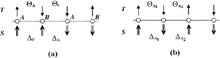
Figure 1: Two schemes to approach the dimer phases. The single and double arrow lines represent T and S, respectively. Two parallel arrows represent FM channel, and two antiparallel arrows represent AFM channel.

One can find, for the scheme (a), the spin $S$ chain and the pseudospin $T$ chain are the same object mathematically: dimerized chain with alternating FM and AFM bonds. For the spin $S$ part, we can divide it into two sublattices $A$ and $B$ by assuming that the translational invariance is broken simultaneously. In fact, the period length of the chain is doubled due to the spin-Peierles phenomenon. We use two sets of Schwinger bosons $\left(a,b\right)$ and $\left(c,d\right)$ to represent spins on the sublattices $A$ and $B$ respectively and choose the unit cell to be composed of two lattice sites with one for sublattice $A$ and another for sublattice $B$. Then the Fourier transformations read

$$\binom{a_{j}}{b_{j}} =\frac{1}{\sqrt{N}}\sum_{k}e^{ikR_{j}}\binom{a_{k}}{b_{k}},$$ (11a)

$$\binom{c_{j+\delta}}{d_{j+\delta}} =\frac{1}{\sqrt{N}}\sum_{k}e^{ik\left(R_{j}+\delta\right)}\binom{c_{k}}{d_{k}},$$ (11b)

$$R_{j} =j,\ \delta=\frac{1}{2}.$$ (11c)

Supposed nonzero real mean fields are

$$\Delta_{A} =\left\langle\frac{1}{2}\left(a_{j}d_{j+\delta}-b_{j}c_{j+\delta}\right)\right\rangle,$$ (12a)

$$\Delta_{F} =\left\langle\frac{1}{2}\left(a_{j}^{{\dagger}}c_{j-\delta}+b_{j}^{{\dagger}}d_{j-\delta}\right)\right\rangle.$$ (12b)

The Lagrangian multipliers, $$\lambda_{j,S}^{(A)} \lambda_{j,S}^{(B)} S$$ and , are imposed to realize the constraints on the spin by adding the term in the total Hamiltonian,

$$\sum_{j}\lambda_{j,S}^{(A)}\left(a_{j}^{{\dagger}}a_{j}+b_{j}^{{\dagger}}b_{j}-2S\right)$$

$$+\sum_{j}\lambda_{j,S}^{(B)}\left(c_{j+\delta}^{{\dagger}}c_{j+\delta}+d_{j+\delta}^{{\dagger}}d_{j+\delta}-2S\right).$$ (13)

For a mean field approach we take $\lambda_{j,S}^{(A)}=\lambda_{j,S}^{(B)}=\lambda_{S}.$ After the Fourier transform, we introduce the Nambu spinor in the momentum space, $\phi_{k}^{\dagger}=\left(a_{k}^{\dagger},b_{-k},c_{k}^{\dagger},d_{-k},a_{-k},b_{k}^{\dagger},c_{-k},d_{k}^{\dagger}\right).$ One can arrive at the mean-field Hamiltonian for the spin $S$ chain in compact form,

$$H^{S}=\frac{1}{2}\sum_{k}\phi_{k}^{\dagger}M^{S}\phi_{k}+\varepsilon_{0}^{S},$$ (14)

where

$$\varepsilon_{0}^{S}=N\left[\left(\Theta_{F}^{2}+y\right)\Delta_{A}^{2}+\left(\Theta_{A}^{2}-y\right)\Delta_{F}^{2}\right]-2N\lambda_{S}(2S+1),$$ (15)

and the matrix $M^{S}$ is constructed by the Kronecker products of the Pauli matrices,

$$M^{S} =\lambda_{S}\sigma_{0}\otimes\sigma_{0}\otimes\sigma_{0}$$

$$+j_{A,S}\cos\frac{k}{2}\ \sigma_{0}\otimes\sigma_{y}\otimes\sigma_{y}+j_{A,S}\sin\frac{k}{2}\ \sigma_{0}\otimes\sigma_{x}\otimes\sigma_{y}$$

$$-j_{F,S}\cos\frac{k}{2}\ \sigma_{0}\otimes\sigma_{x}\otimes\sigma_{z}+j_{F,S}\sin\frac{k}{2}\ \sigma_{0}\otimes\sigma_{y}\otimes\sigma_{z}$$ (16)

with $j_{A,S}=\left(\Theta_{F}^{2}+y\right)\Delta_{A}/2,\ j_{F,S}=\left(\Theta_{A}^{2}-y\right)\Delta_{F}/2,\ j_{A,T}=\left(\Delta_{F}^{2}+x\right)\Theta_{A}/2,\$and $j_{F,T}=\left(\Delta_{A}^{2}-x\right)\Theta_{F}/2$. Then we can read out the spectra from the poles of the bosonic Matsubara Green’s function ($8\times 8$ matrix),

$$G^{S}\left(k,i\omega_{n}\right)=\left(i\omega_{n}\sigma_{z}\otimes\sigma_{0}\otimes\sigma_{z}-M^{S}\right)^{-1}$$ (17)

where $\omega_{n}=n\pi/\beta$ ($n$ is an integer and $\beta$ is the inverse temperature). Similarly we repeat the mean field calculation on the pseudospin $T$ chain. Both the spin and the pseudospin chains have two spectra, which read

$$\omega_{\alpha,\nu}\left(k\right)=\sqrt{\lambda_{\alpha}^{2}-j_{A,\alpha}^{2}+j_{F,\alpha}^{2}+2\nu j_{F,\alpha}\Omega_{\alpha}\left(k\right)},$$ (18)

where $\alpha=(S,T)$, $\nu=\mp$, and $\Omega_{\alpha}\left(k\right)=\sqrt{\lambda_{\alpha}^{2}-j_{A,\alpha}^{2}\cos^{2}k}$. The lower quasiparticle spectrum $\omega_{\alpha,-}\left(k\right)$ is found to be gapped at $k=\pm\pi/2$, which is related to the physical gap by the peak of the imaginary part of the dynamic spin susceptibility.A And the gap is also true for half integer spin (or pseudospin).SXZ ; MYK By optimizing the total free energy

$$F=\varepsilon_{0}-\frac{1}{\beta}\sum\limits_{k,\alpha,\nu}\ln\left[n_{B}\left(\omega_{\alpha,\nu}\left(k\right)\right)\left\{n_{B}\left(\omega_{\alpha,\nu}\left(k\right)\right)+1\right\}\right],$$ (19)

where $n_{B}(\omega)$ is the Bose-Eienstein distribution and

$$\varepsilon_{0} =N[3\left(\Theta_{A}^{2}\Delta_{F}^{2}+\Theta_{F}^{2}\Delta_{A}^{2}\right)+2xy+\left(\Delta_{A}^{2}-\Delta_{F}^{2}\right)y$$

$$+\left(\Theta_{A}^{2}-\Theta_{F}^{2}\right)x-2\lambda_{S}(2S+1)-2\lambda_{T}(2T+1)],$$ (20)

a set of the mean field equations are established,

$$W\left(\widetilde{j}_{A,S},\widetilde{j}_{F,S}\right) =2S+1,$$ (21a)

$$W\left(\widetilde{j}_{A,T},\widetilde{j}_{F,T}\right) =2T+1,$$ (21b)

$$X\left(\widetilde{j}_{A,S},\widetilde{j}_{F,S}\right) =\Delta_{A},$$ (21c)

$$X\left(\widetilde{j}_{A,T},\widetilde{j}_{F,T}\right) =\Theta_{A},$$ (21d)

$$Y\left(\widetilde{j}_{A,S},\widetilde{j}_{F,S}\right) =\Delta_{F},$$ (21e)

$$Y\left(\widetilde{j}_{A,T},\widetilde{j}_{F,T}\right) =\Theta_{F},$$ (21f)

$$\frac{\left(\Theta_{F}^{2}+y\right)\Delta_{A}}{\widetilde{j}_{A,S}} =\frac{\left(\Theta_{A}^{2}-y\right)\Delta_{F}}{\widetilde{j}_{F,S}}=2\lambda_{S},$$ (21g)

$$\frac{\left(\Delta_{F}^{2}+x\right)\Theta_{A}}{\widetilde{j}_{A,T}} =\frac{\left(\Delta_{A}^{2}-x\right)\Theta_{F}}{\widetilde{j}_{F,T}}=2\lambda_{T},$$ (21h)

where we have defined integrals (the symbols with wave decoration means dimensionless quantities, $$\widetilde{j}_{A,\alpha}=j_{A,\alpha}/\lambda_{\alpha},\widetilde{j}_{F,\alpha}=j_{F,\alpha}/\lambda_{\alpha},\widetilde{\Omega}_{\alpha}=\Omega_{\alpha}/\lambda_{\alpha} \frac{1}{N} \sum_{k}\rightarrow\int\frac{dk}{2\pi}$$, and we have substituted the sum with integral: ),

$$W(\widetilde{j}_{A,\alpha},\widetilde{j}_{F,\alpha}) =\int\frac{dk}{2\pi}\sum_{\nu=\mp}\left(1+\frac{\nu\widetilde{j}_{F,\alpha}}{\widetilde{\Omega}_{\alpha}}\right)\frac{\coth\frac{\beta\omega_{\alpha,\nu}}{2}}{2\widetilde{\omega}_{\alpha,\nu}},$$ (22a)

$$X(\widetilde{j}_{A,\alpha},\widetilde{j}_{F,\alpha}) =\int\frac{dk}{2\pi}\sum_{\nu=\mp}\left(1+\frac{\nu\widetilde{j}_{F,\alpha}\cos^{2}k}{\widetilde{\Omega}_{\alpha}}\right)\frac{\coth\frac{\beta\omega_{\alpha,\nu}}{2}}{4\widetilde{\omega}_{\alpha,\nu}},$$ (22b)

$$Y(\widetilde{j}_{A,\alpha},\widetilde{j}_{F,\alpha}) =-\int\frac{dk}{2\pi}\sum_{\nu=\mp}\left(\widetilde{j}_{F,\alpha}+\nu\widetilde{\Omega}_{\alpha}\right)\frac{\coth\frac{\beta\omega_{\alpha,\nu}}{2}}{4\widetilde{\omega}_{\alpha,\nu}}.$$ (22c)

III Phase diagram

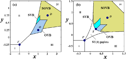
Figure 2: (Color online) Phase diagrams for: (a) $S=1,T=1/2$; (b) $S=1/2,T=1/2$. The uniform phases are: I for S-FM and T-FM; II for S-AFM and T-FM; III for S-FM and T-AFM; IV for S-AFM and T-AFM. The SU(4) gapless region is quoted from Ref. I The special points are: $F$ - the FM point; $D$ - the dimer point, $S$ - the SU(4) symmetric point, and $O$ - the representative point of OVB phase. Please see details in the text.

For the transition-metal oxides, the pseudospin is usually one half, i. e. $T=1/2$, reflecting two choices of unfrozen $e_{g}$ or $t_{2g}$ orbitals.TN ; KHO Spin-gap materials, Na₂Ti₂Sb₂O and NaV₂O₅, are related to the $S=1/2$ case in the model of Eq. (1),PSK ; Fujii while cubic vanadates, LaVO₃ and YVO₃, are related to $S=1$ case due to large Hund’s coupling.KHO ; MFM

The phase diagrams are obtained by solving the mean field equations numerically at zero temperature. Fig. 2(a) shows the case for $S=1$ and $T=1/2$. We found three dimer phases: (1) the OVB phase with $\Theta_{A}=\sqrt{3}/2,\Theta_{F}=0,\Delta_{A}\neq 0$ and $\Delta_{F}\neq 0$; (2) the SVB phase with $\Theta_{A}\neq 0,\Theta_{F}\neq 0,\Delta_{A}=\sqrt{2}$ and $\Delta_{F}=0$; (3) the SOVB phase with $\Theta_{A}=\sqrt{3}/2,\Theta_{F}=0,\Delta_{A}=\sqrt{2}$ and $\Delta_{F}=0$. As expected, the point $O$: $(x,y)=(1,1/4)$ lies in the OVB phase region. At the mean field level, the dimer phases are captured by the staggered non-zero AFM mean fields $\Theta_{A}$ and/or $\Delta_{A}$, which provide a perfect dimer picture of spin and/or pseudospin in the whole phase regions. The reason for this maybe lies in two: the mean field treatment omits part of quantum fluctuations; the dimerization effect is very strong in such a system at least at zero temperature. In fact, TMRG has confirmed the orbital dimerization at the point $O$: $\left(x,y\right)=\left(1,1/4\right)$ since the correlation function $\left\langle\mathbf{T}_{m}\cdot\mathbf{T}_{m+1}\right\rangle$ extrapolates to $-3/8$ per bond at zero temperature, although this point is not exactly soluble.SK And the OVB phase is quite robust even when the anisotropy, Hund’s coupling, and atomic spin-orbit interaction are taken into account for cubic vanadates and relevant systems.SXZ ; HKO We also guess these dimer phases may survive in two dimensions, although no rigorous soluble point can be referred to. A dimerized OVB configuration in two dimensions has been proposed and checked by the spin-wave theory in Ref. SXZ , which indeed exhibits lower energy than the uniform phases. However it is an interesting problem whether SOVB can survive in two dimensions.

Fig. 2(b) shows the case for $S=1/2$ and $T=1/2$. In Fig. 2(b), the $SU(4)$ gapless region is quoted from Ref. I . We found the SVB and OVB phases still occupy two areas that are sandwiched between the SOVB and $SU(4)$ gapless region. The three dimer phases with corresponding mean fields are: (1) the OVB phase with $\Theta_{A}=\sqrt{3}/2,\Theta_{F}=0,\Delta_{A}\neq 0$ and $\Delta_{F}\neq 0$; (2) the SVB phase with $\Theta_{A}\neq 0,\Theta_{F}\neq 0,\Delta_{A}=\sqrt{3}/2$ and $\Delta_{F}=0$; (3) the SOVB phase with $\Theta_{A}=\sqrt{3}/2,\Theta_{F}=0,\Delta_{A}=\sqrt{3}/2$ and $\Delta_{F}=0$. Previous works ignored the SVB and OVB phases.PSK ; I And there is a $S$-AFM and $T$-AFM phase region from the point of view of SBMFT.

The result here in fact suggests that the spin-orbit coupling of $SU(2)\times SU(2)$ type plays the roles of the intrinsic spin-Peierls and orbital-Peierls mechanisms. The SVB formation in this $1D$ model is an example that expresses the concept of orbitally driven Peierls state.Khomskii But notice we did not consider the lattice distortion here. For spin $S=1$, the SVB phase is harder to realize since the region shrinks.

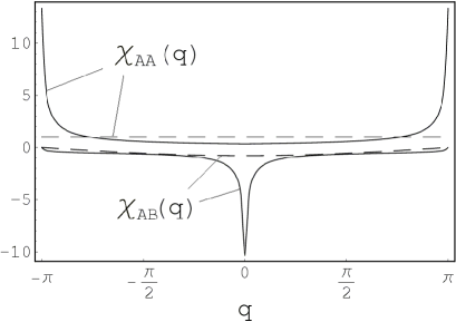
Figure 3: Static spin susceptibilities for $S=1$ and $T=1/2$ at the OVB point $O$: $(x,y)=(1,1/4)$ (solid line) and the dimer point $D$: $(2,3/4)$ (dashed line).

IV Susceptibility

The spin structures of the dimer phases are detectable by spin susceptibility. Let us consider the spin susceptibility (the psedospin case is handled in the same way). We can define the spin density waves on sublattices $A$ and $B$ (due to the rotational symmetry, we only consider $z$ component of the spin),

$$S_{A}^{z}\left(q\right) =\frac{1}{\sqrt{N}}\sum e^{-iqR_{j}}S_{A,j}^{z},$$ (23a)

$$S_{B}^{z}\left(q\right) =\frac{1}{\sqrt{N}}\sum e^{-iq\left(R_{j}+\delta\right)}S_{B,j+\delta}^{z}.$$ (23b)

The spin susceptibility contains contributions from both the intra-sublattice and inter-sublattice fluctuations,

$$\chi\left(q\right) =\frac{1}{N}\sum_{m,n\in A,B}\left\langle S_{m}^{z}S_{n}^{z}\right\rangle e^{iq(R_{m}-R_{n})}$$

$$=\chi_{AA}\left(q\right)+\chi_{AB}\left(q\right)+\chi_{BA}\left(q\right)+\chi_{BB}\left(q\right).$$ (24)

In Matsubara formalism, the intra-sublattice and inter-sublattice contributions read

$$\chi_{AA}\left(q,\tau\right) =\left\langle S_{A}^{z}\left(q,\tau\right)S_{A}^{z}(-q,0)\right\rangle$$

$$=\frac{1}{4}\int_{-\pi}^{\pi}\frac{dk}{2\pi}[2G_{55}^{S}\left(-k,\tau\right)G_{11}^{S}\left(k+q,\tau\right)$$

$$\qquad\qquad-G_{56}^{S}\left(-k,\tau\right)G_{12}^{S}\left(k+q,\tau\right)$$

$$\qquad\qquad-G_{21}^{S}\left(-k,\tau\right)G_{65}^{S}\left(k+q,\tau\right)],$$ (25a)

$$\chi_{AB}\left(q,\tau\right) =\left\langle S_{A}^{z}\left(q,\tau\right)S_{B}^{z}(-q,0)\right\rangle$$

$$=\frac{1}{4}\int_{-\pi}^{\pi}\frac{dk}{2\pi}[2G_{57}^{S}\left(-k,\tau\right)G_{13}^{S}\left(k+q,\tau\right)$$

$$\qquad\qquad-G_{58}^{S}\left(-k,\tau\right)G_{14}^{S}\left(k+q,\tau\right)$$

$$\qquad\qquad-G_{23}^{S}\left(-k,\tau\right)G_{67}^{S}\left(k+q,\tau\right)],$$ (25b)

respectively, where the Green’s function in imaginary time $$\tau$$ is related to Eq. (17) by

$$G^{S}\left(k,\tau\right)=\frac{1}{\beta}\sum_{n}e^{-i\omega_{n}\tau}G^{S}\left(k,i\omega_{n}\right).$$ (26)

The numerical solutions of the static spin susceptibilities, $\chi_{AA}\left(q,\tau=0^{+}\right)$ and $\chi_{AB}\left(q,\tau=0^{+}\right)$, for $S=1$ and $T=1/2$ at the OVB point $O$: $(x,y)=(1,1/4)$ and the dimer point $D$: $(2,3/4)$ are shown in Fig. 3. At the OVB point $O$, the static spin susceptibilities exhibit finite sharp peaks at $q=\pi$ for $\chi_{AA}\left(q,\tau\right)$ and $q=0$ for $\chi_{AB}\left(q,\tau\right)$ reflecting the strong AFM fluctuation among sites in sublattice $A$ (or $B$) and FM fluctuation between sites in sublattice $A$ and sites in sublattice $B$. The finite peaks also indicate no long-range order exists at zero temperature. While there is no sharp peak at the dimer point $D$, since the formation of spin singlets leads to dispersionless spin spectra, $\omega_{S,-}\left(k\right)=\omega_{S,+}\left(k\right)=\sqrt{\lambda_{S}^{2}-j_{A,S}^{2}}$. The spin susceptibilities at the OVB point $O$ and the dimer point $D$ characterize the whole OVB region and SOVB region respectively. As we go from OVB phase to SVB phase, the spin and pseudospin change their roles. In SOVB phase, the sharp peaks will disappear for both spin and pseudospin. Thus the three dimer phases are well characterized by the spin and pseudospin susceptibilities and distinguishable experimentally. A recent neutron scattering experiment of YVO₃ has provided a tentative proof of the OVB.U

V Conclusion

In conclusion, we have employed SBMFT to study the valence bond states as well as uniform FM and AFM states in the $1D$ $SU(2)\times SU(2)$ spin-orbital model. The phase diagrams are constructed by comparing the ground energies of the proposed possible states. In the valence bond states the translational invariance is broken in space, FM and AFM parameters compete with each other and are determined self-consistently. Specifically, two sublattices are introduced to approach the three dimerized SVB, OVB and SOVB phases by SBMFT. We clarified how to capture properly the low temperature properties of such a system by SBMFT. The main result of the paper is that the SVB and OVB have lower energy than the SOVB in some regions. These consequences reveal that the $SU(2)\times SU(2)$ type spin-orbit coupling can provide both spin-Peierls and orbital-Peierls mechanisms. The results still should be compared with other phases including those with translational invariance. Static spin and pseudospin susceptibilities had been calculated in the present theory and are available to distinguish spin-singlet and orbital-singlet formations in real materials.

This work was supported by the Research Grant Council of Hong Kong (No.: HKU/7109/02P and 7038/04P)

References

• (1) Y. Tokura and N. Nagaosa, Science 288, 462 (2000).
• (2) I. Kugel and D. I. Khomskii, Sov. Phys. JETP lett. 37, 725 (1973); Sov. Phys. Usp. 25, 231 (1982).
• (3) T. M. Rice, Spectroscopy of Mott Insulators and Correlated Metals, edited by A. Fujimori and Y. Tokura (Springer, Berlin, 1995).
• (4) D. P. Arovas and A. Auerbach, Phys. Rev. B 52, 10114 (1995).
• (5) S. K. Pati, R. R. P. Singh and D. I. Khomskii, Phys. Rev. Lett. 81, 5406 (1998).
• (6) Y. Fujii, H. Nakao, T. Yosihama, M. Nishi, K. Nakajima, K. Kakurai, M. Isobe, Y. Ueda and H. Sawa, J. Phys. Soc. Jpn. 66, 326 (1997).
• (7) G. Khaliullin, P. Horsch and A. M. Oles, Phys. Rev. Lett. 86, 3879 (2001).
• (8) C. Itoi, S. Qin and I. Affleck, Phys. Rev. B 61, 6747 (2000).
• (9) W. Zheng and J. Oitmaa, Phys. Rev. B 64, 014410 (2001).
• (10) A. K. Kolezhuk and H. -J. Mikeska, Phys. Rev. Lett. 80, 2709 (1998); K. Itoh, J. Phys. Soc. Jpn. 68, 322 (1999).
• (11) Y. Q. Li, M. Ma, D. N. Shi and F. C. Zhang, Phys. Rev. Lett. 81, 3527 (1998).
• (12) S. Q. Shen, X. C. Xie and F. C. Zhang, Phys. Rev. Lett. 88, 27201 (2002).
• (13) J. Sirker and G. Khaliullin, Phys. Rev. B 67, 100408 (2003).
• (14) C. Ulrich, G. Khaliullin, J. Sirker, M. Reehuis, M. Ohl, S. Miyaska, Y. Tokura and B. Keimer, Phys. Rev. Lett. 91, 257202 (2003).
• (15) A. Auerbach, Interacting Electrons and Quantum Magnetism (Springer-Verlag, New York, 1994).
• (16) A. Auerbach and D. Arovas, Phys. Rev. Lett. 61, 617 (1988); Phys. Rev. B. 38, 316 (1988).
• (17) S. Sarker, C. Jayaprakash, H. R. Krishnamurthy and M. Ma, Phys. Rev. B. 40, 5028 (1989).
• (18) G. M. Zhang and S. Q. Shen, Phys. Rev. Lett. 87, 157201(2001); S. Q. Shen and G. M. Zhang, Europhys. Lett. 57, 274 (2002).
• (19) H. A. Ceccatto, C. J. Gazza and A. E. Trumper, Phys. Rev. B 47, 12329 (1993).
• (20) A. E. Trumper, L. O. Manuel, C. J. Gazza and H. A. Ceccatto, Phys. Rev. Lett. 78, 2216 (1997).
• (21) S. Q. Shen, Phys. Rev. B 66, 214516 (2002); P. Li and S. Q. Shen, N. J. Phys. 6, 160 (2004).
• (22) H. Manaka, I. Yamada, T. Kikuchi, K. Morishita and K. Iio, J. Phys. Soc. Jpn. 70, 2509 (2001).
• (23) T. Mizokawa and A. Fujimori, Phys. Rev. B 54, 5368 (1996); F. Mila, R. Shiina, F. C. Zhang, A. Joshi, M. Ma, V. Anisimov and T. M. Rice, Phys. Rev. Lett. 85, 1714 (2000).
• (24) P. Horsch, G. Khaliullin and A. M. Oles, Phys. Rev. Lett. 91, 257203 (2003).
• (25) D. I. Khomskii and T. Mizokawa, Phys. Rev. Lett. 94, 156402 (2005).