Quantum simulation of manybody effects in steady-state nonequilibrium: electron-phonon coupled quantum dots

Abstract

We develop a mapping of quantum steady-state nonequilibrium to an effective equilibrium and solve the problem using a quantum simulation technique. A systematic implementation of the nonequilibrium boundary condition in steady-state is made in the electronic transport on quantum dot structures. This formulation of quantum manybody problem in nonequilibrium enables the use of existing numerical quantum manybody techniques. The algorithm coherently demonstrates various transport behaviors from phonon-dephasing to $I-V$ staircase and phonon-assisted tunneling.

Electronic transport in nanoscale devices has recently attracted much attention for its tremendous impact in modern electronics. In nanoscale devices, fundamental understanding of quantum physics holds the key to a breakthrough in the field. One of the central issues is to understand the increasing interplay of quantum manybody effect and the high-bias nonequilibrium.

Despite the intense research in the nanoscale transport, most of the theoretical tools are based on the Green function technique datta_book ; wingreen ; rammer ; datta_prb , and powerful numerical equilibrium techniques, which have been essential in quantum manybody theories, have not been useful due to the lack of nonequilibrium formulation. Application of such well-established numerical techniques, such as quantum Monte Carlo (QMC) method bss , to nonequilibrium with full quantum manybody effects will provide a breakthrough in the field. The goal of this work is to formulate a general scheme of combining the nonequilibrium theory with numerical quantum manybody techniques via a mapping of a nonequilibrium system to an effective equilibrium. This method applied in electron-phonon coupled quantum dot systems demonstrates various transport behavior such as the phonon dephasing, phonon-assisted tunneling, $I-V$ staircase in a single framework. The formulation shown is applicable to other numerical techniques, such as nemerical renormalization group, exact diagonalization, etc.

Conventional diagrammatic theory is founded in adiabatic turn-on of interaction. Here we begin from a very different point that a steady-state nonequilibrium possesses the time-invariance, where the transient states are damped out. With this observation, Hershfield hershfield has shown the existance of an effective Hamiltonian which builds the nonequilibrium ensemble in steady-state. The ensemble can be represented in terms of a modified partition function $Z_{\rm noneq}$ for nonequilibrium as

$$Z_{\rm noneq}={\rm Tr}e^{-\beta(\hat{H}-\hat{Y})}\quad\mbox{with}\quad\beta=1/T,$$ (1)

where $\hat{H}$ is the usual Hamiltonian operator for the whole system including the source (left, $L$), drain (right, $R$) reservoirs and quantum dot (QD) (see FIG. 1 (a)). The additional operator $\hat{Y}$ accounts for the boundary condition of chemical potential difference in the two reservoirs, given by the bias $\Phi$. Once the bias operator $\hat{Y}$ is constructed, one can apply the usual equilibrium QMC technique bss to $\hat{H}_{\rm noneq}=\hat{H}-\hat{Y}$ as if $\hat{H}_{\rm noneq}$ describes an equilibrium. To obtain $I-V$ characteristics, for instance, one simply needs to evaluate the expectation value of the current operator $\hat{I}$,

$$I=\frac{{\rm Tr}\,\,\hat{I}e^{-\beta(\hat{H}-\hat{Y})}}{{\rm Tr}\,\,e^{-\beta(\hat{H}-\hat{Y})}}=\frac{ie}{h}\sum_{k\sigma}\frac{t_{Lk}}{\sqrt{\Omega}}\left[\langle c^{\dagger}_{Lk\sigma}d_{\sigma}\rangle-\langle d^{\dagger}_{\sigma}c_{Lk\sigma}\rangle\right],$$ (2)

where $c^{\dagger}_{Lk\sigma}$ ($c_{Lk\sigma}$) is the electron creation (annihilation) operator of spin $\sigma$, the $k$-th continuum state in the $L$-reservoir, $d^{\dagger}_{\sigma}$ ($d_{\sigma}$) the operator for QD state, and $t_{L}$ the hopping integral (with the volume factor $\Omega$) between the QD and the $L$-reservoir (see FIG. 1(a)).

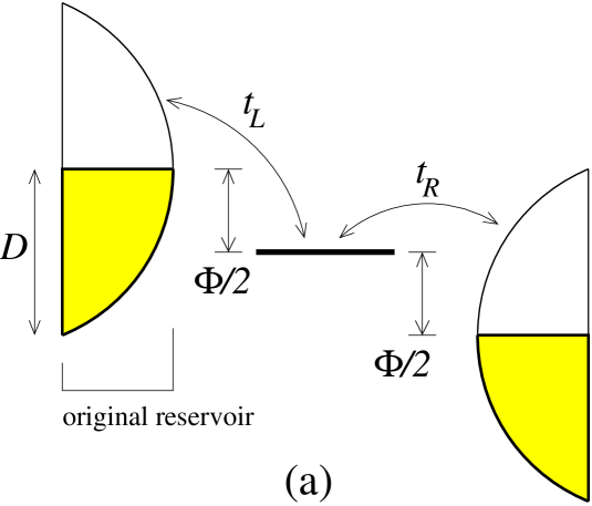
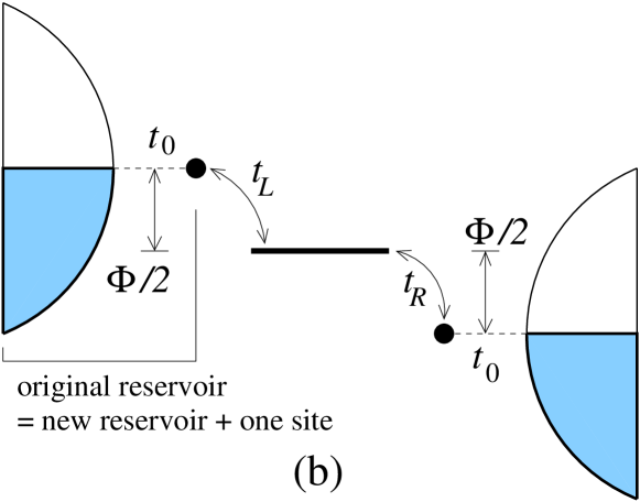
Figure 1: (a) Schematic diagram of a quantum transport device. The source and drain reservoirs are biased by a chemical potential difference $\Phi$. The quantum dot (QD) level is set in the middle for simplicity. (b) Each reservoir is mapped to a single site and a new reservoir. The three discrete sites for the QD and $L$- and $R$-sites are treated in fully quantum mechanical manner.

The central challenge is to construct the bias operator $\hat{Y}$. Once a nonequilibrium ensemble is established via $e^{-\beta(\hat{H}-\hat{Y})}$, the subsequent motion is governed by the time evolution operator $e^{-i\hat{H}t}$. Therefore the bias operator $\hat{Y}$ must satisfy the commutation relation $[\hat{H},\hat{Y}]=0$. Hershfield hershfield has shown that $\hat{Y}$ can be written in terms of the scattering state operator $\psi^{\dagger}_{\alpha k\sigma}$ ($\alpha=L,R$) as localized

$$\hat{Y}=-\frac{\Phi}{2}\sum_{k\sigma}\left(\psi^{\dagger}_{Lk\sigma}\psi_{Lk\sigma}-\psi^{\dagger}_{Rk\sigma}\psi_{Rk\sigma}\right).$$ (3)

The scattering state creation operator $\psi^{\dagger}_{\alpha k\sigma}$ satisfies the Lippman-Schwinger equation in the operator form,

$$[\hat{H},\psi^{\dagger}_{\alpha k\sigma}]=\epsilon_{\alpha k}\psi^{\dagger}_{\alpha k\sigma}+i\eta(\psi^{\dagger}_{\alpha k\sigma}-c^{\dagger}_{\alpha k\sigma}),$$ (4)

with $\epsilon_{\alpha k}$ the asymptotic continuum energy and $\eta$ an infinitesimal convergence factor.

There are two main issues to implement the above nonequilibrium ensemble. First, to systematically construct $\hat{Y}$, the scattering state is expanded in terms of interaction as $\psi^{\dagger}_{\alpha k\sigma}=\sum_{n}\psi^{\dagger}_{\alpha k\sigma,n}$ hershfield satisfying

$$[\hat{V},\psi^{\dagger}_{\alpha k\sigma,n-1}]=(\epsilon_{\alpha k}+i\eta)\psi^{\dagger}_{\alpha k\sigma,n}-[\hat{H}_{0},\psi^{\dagger}_{\alpha k\sigma,n}],$$ (5)

where the total Hamiltonian $\hat{H}=\hat{H}_{0}+\hat{V}$. $\hat{H}_{0}$ is the non-interacting and $\hat{V}$ the interacting part of the Hamiltonian. The second and more serious issue is the non-locality of the operator $\hat{Y}$. Since the one-particle eigenstate of the total Hamiltonian is delocalized in space, the bi-products $\psi^{\dagger}_{\alpha k\sigma}\psi_{\alpha k\sigma}$ in $\hat{Y}$ produce non-local terms even if the model Hamiltonian $\hat{H}$ is given with local interactions. Despite the great potential of Hershfield’s paper hershfield , only limited developments schiller ; bokes have been made so far due to such difficulties.

To make the following discussions concrete, let us consider an example: electron-phonon (el-ph) coupled QD connected to two $L$, $R$-reservoirs. Spinless Hamiltonian for the system reads $\hat{H}=\hat{H}_{0}+\hat{V}=\hat{H}^{el}_{0}+\hat{H}^{ph}_{0}+\hat{V}$,

$$\hat{H}^{el}_{0} = \sum_{\alpha k}\epsilon_{\alpha k}c^{\dagger}_{\alpha k}c_{\alpha k}+\epsilon_{d}d^{\dagger}d+\sum_{\alpha k}\frac{t_{\alpha k}}{\sqrt{\Omega}}\left(d^{\dagger}c_{\alpha k}+h.c.\right)$$

$$\hat{H}^{ph}_{0} = \frac{1}{2}\left(p^{2}+\omega_{ph}^{2}\varphi^{2}\right),\hat{V}=\alpha\varphi(d^{\dagger}d-\langle d^{\dagger}d\rangle),$$ (6)

where $\varphi$ is phonon amplitude, $p$ its conjugate momentum, $\omega_{ph}$ phonon frequency, and $\alpha(\equiv g\sqrt{2\omega_{ph}})$ the el-ph coupling constant. As shown in FIG. 1(a), we model the continuum states to be shifted with the bias, i.e., $\epsilon_{Lk}=\epsilon_{k}+\Phi/2$ and $\epsilon_{Rk}=\epsilon_{k}-\Phi/2$. We set the particle-hole symmetric QD level ($\epsilon_{d}=0$) for simplicity.

Here we propose that we capture important manybody effects by isolating the leading order non-local interactions as follows. We make two observations in $\hat{H}-\hat{Y}$. First, the QD level is modulated by phonons as $\epsilon_{d}(\varphi)=\epsilon_{d}+\alpha\varphi$. The fluctuation of the QD level results in dephasing of the current. Second, the hopping out of the QD to the continuum is effectively modified as $\epsilon_{d}(\varphi)$ is driven in and out of resonance with respect to the reservoir chemical potentials. As will be discussed later, fluctuations in the hopping integral result in phonon satellites in current. With these observations, we isolate the first path of hopping from the QD by rewriting the each continuum as a fictitious site and a new continuum, as depicted in FIG. 1(b). We then treat the coupling between the three sites fully quantum mechanically and make mean-field approximations to terms involving the continuum states. This procedure can be systematically improved by inserting additional fictitious reservoir sites to a better non-local approximation.

We have used a semi-circular density of state (DOS) for the continua, $N(\epsilon_{\alpha})=2\sqrt{D^{2}-\epsilon_{\alpha}^{2}}/\pi D^{2}$, with the Fermi energy $\epsilon_{F}=D$. The semi-circular DOS is particularly useful since, with the intra-reservoir hopping $t_{0}=D/2$ (see FIG. 1), the resulting new DOS is identical to the original DOS. In the non-interacting limit ($\hat{V}=0$), the scattering state can be readily obtained by expanding $\psi^{\dagger}_{\alpha k}$ in terms of the basis states in Eq. (4) as

$$\psi^{\dagger}_{Lk,0}=c^{\dagger}_{Lk}+\frac{t_{0}}{\sqrt{\Omega}}\sum_{\beta}g^{0}_{L,\beta}(\epsilon_{Lk})c^{\dagger}_{\beta},$$ (7)

where $\beta=Lk^{\prime},L,d,R,Rk^{\prime}$ with $L,R$ denoting the fictitious reservoir sites, and $Lk^{\prime},Rk^{\prime}$ new continuum states. $c^{\dagger}_{d}$ is the same as $d^{\dagger}$. $g^{0}_{L\beta}(\epsilon)$ are retarded Green functions propagating from state $L$ to $\beta$. $\psi^{\dagger}_{Rk,0}$ are similarly obtained. From Eq. (2), one can recover the Landauer-Büttiker formula in the non-interacting limit.

We expand the scattering states up to harmonic el-ph coupling via Eq. (5). With $[\hat{V},\psi^{\dagger}_{Lk,0}]=(t_{0}/\sqrt{\Omega})\alpha\varphi g^{0}_{Ld}(\epsilon_{Lk})d^{\dagger}$ and $\psi^{\dagger}_{\alpha k,1}$ expanded as

$$\psi^{\dagger}_{Lk,1}=\varphi\sum_{\beta}a^{Lk}_{\beta}c^{\dagger}_{\beta}+p\sum_{\beta}b^{Lk}_{\beta}c^{\dagger}_{\beta},$$ (8)

one obtains explicit expressions for $a_{\beta},b_{\beta}$ after a straightforward calculation. Up to the linear order of $(\varphi,p)$ we obtain $\hat{Y}=\hat{Y}_{0}+\hat{Y}_{1}$ with $\hat{Y}_{0}=\Phi/2\sum_{k}(\psi^{\dagger}_{Lk0}\psi_{Lk0}-\psi^{\dagger}_{Rk0}\psi_{Rk0})$, $\hat{Y}_{1}=\Phi/2\sum_{k}(\psi^{\dagger}_{Lk0}\psi_{Lk1}+\psi^{\dagger}_{Lk1}\psi_{Lk0}-\psi^{\dagger}_{Rk0}\psi_{Rk1}-\psi^{\dagger}_{Rk1}\psi_{Rk0})$. Now we make a mean-field approximations ($\varphi=0$) on the terms which involve the continuum states $Lk^{\prime}$, $Rk^{\prime}$. Projected onto the discrete basis $(L,d,R)$, $\hat{Y}_{1}$ reads

$$\hat{Y}_{1}=\varphi\hat{A}+p\hat{B}=\sum_{\beta,\gamma=L,d,R}\left(\varphi A_{\beta\gamma}+pB_{\beta\gamma}\right)c^{\dagger}_{\beta}c_{\gamma},$$ (9)

where the $3\times 3$ matrix $A$ is written as

$$A_{\beta\gamma} = \frac{\Phi}{2}\sum_{k}\left[a^{Lk}_{\beta}\left(g^{0}_{L\gamma}(\epsilon_{Lk})\right)^{*}+g^{0}_{L\beta}(\epsilon_{Lk})\left(a^{Lk}_{\gamma}\right)^{*}\right.$$ (10)

$$\left.-a^{Rk}_{\beta}\left(g^{0}_{R\gamma}(\epsilon_{Rk})\right)^{*}-g^{0}_{R\beta}(\epsilon_{Rk})\left(a^{Rk}_{\gamma}\right)^{*}\right],$$

and $B$ is given by replacing $a^{\alpha k}_{\beta}$ by $b^{\alpha k}_{\beta}$.

We now sample the ensemble by treating $\hat{H}_{\rm noneq}$ as in conventional QMC bss . We express the Boltzmann factor into the Trotter breakup bss , ${\rm Tr}\,\exp(-\beta\hat{H}_{\rm noneq})={\rm Tr}[\exp(-\Delta\tau\hat{H}_{\rm noneq})]^{N}$ with $\beta=N\Delta\tau$. The three discrete sites ($L,d,R$) are considered as a generalized impurity and the Hirsch-Fye algorithm hirsch is employed to integrate out the continuum states which are incorporated in the non-interacting Green function $G^{0}_{\beta\gamma}(i\omega_{n})$ at the Matsubara imaginary frequency $\omega_{n}=(2n+1)\pi/\beta$ as

$$G^{0}_{\beta\gamma}(i\omega_{n})=\!\!\!\sum_{\alpha=L,R;k}\!\frac{g^{0}_{\alpha\beta}(\epsilon_{\alpha k})\left[g^{0}_{\alpha\gamma}(\epsilon_{\alpha k})\right]^{*}}{i\omega_{n}-\epsilon_{\alpha k}+(-)^{\alpha}\Phi/2}+\sum_{m}\frac{c^{m}_{\beta}c^{m*}_{\gamma}}{i\omega_{n}-E_{m}},$$ (11)

where the possible localized states (with the $m$-th energy $E_{m}$ and amplitudes $c^{m}_{\beta}$ for the $\beta$ state) are taken into account. $(-)^{L}\equiv 1,\,(-)^{R}\equiv-1$. The localized states become important in the narrow bandwidth limit.

The main difference from the usual equilibrium QMC is the $p$-term in Eq. (9). Integrating out the canonical momentum $p$ inside time-slices of the Trotter-breakup leads to negele

$$\langle\varphi_{\tau+\Delta\tau}|e^{-\Delta\tau(\frac{1}{2}p^{2}+p\hat{B})}|\varphi_{\tau}\rangle\propto e^{\Delta\tau\left[-\frac{1}{2}\left(\frac{\partial\varphi}{\partial\tau}\right)^{2}+i\hat{B}_{\tau}\frac{\partial\varphi}{\partial\tau}\right]},$$ (12)

where $\hat{B}_{\tau}$ is the electronic operator at the imaginary time $\tau$. Due to the second term $\hat{B}_{\tau}(\partial\varphi/\partial\tau)$, a temporally local update of the phonon field $\varphi_{\tau}$ results in changes in $\hat{B}_{\tau-\Delta\tau},\hat{B}_{\tau},\hat{B}_{\tau+\Delta\tau}$. The apparent broken time-reversal symmetry in the first-order time differentiation $(\partial\varphi/\partial\tau)$ originates from the right-to-left flow of electrons induced by the bias $\Phi$ feldman . The $(\partial\varphi/\partial\tau)$ term also shows bias-induced phonon fluctuations which become crucial in phonon-assisted tunneling tsui . $\Delta\tau=1$ in the following results.

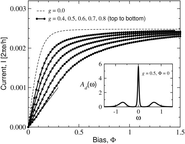
Figure 2: Simulated $I-V$ characteristics in the broad band limit, $D\gg\omega_{ph}$. Parameters are $t_{L}=t_{R}=0.1,\,\omega_{ph}=0.5,\,D=8.0$ and $T=1/32=0.03125$. As the electron-phonon coupling constant $g$ is increased, the current decreased. Non-interacting phonon level aligns to the reservoir Fermi energy at bias $\Phi=2\omega_{ph}=1$. The phonon dephasing effect is so strong that the phonon satellite peak is invisible at all coupling constant while the phonon satellites at zero bias (inset) are clearly separated from the main peak.

$I-V$ curves in the broad band limit ($D\gg\omega_{ph}$) are presented in FIG. 2. The unit of energy is chosen so that the bare phonon level ($\omega_{ph}=0.5$) aligns with the Fermi energy of the $L$-reservoir at unit bias ($\Phi=1$). The current monotonically increased with $\Phi$ at all el-ph coupling constant $g$. The current converges toward the well-known large-band, large-bias limit (dashed line for $g=0$) spin

$$I=\frac{2e}{\hbar}\frac{\Gamma_{L}\Gamma_{R}}{\Gamma_{L}+\Gamma_{R}},\quad\mbox{with\ }\Gamma_{a}=\pi t_{\alpha}^{2}N_{\alpha}(0).$$ (13)

At zero bias, the QD spectral function $A_{d}(\omega)$ with real frequency $\omega$ (see inset) by using the maximum entropy method mem shows that the phonon satellite peaks are clearly separated from the main peak analytic_cont . From this, one might have expected that there would be a double-step $I-V$ characteristics, while the computed curves do not show such distinct features. This suggests that the actual decay rate of the phonon satellite under finite bias ($\Phi\approx 2\omega_{ph}$) is much larger than the zero bias case because the phonon level is now close to a resonance with the reservoir Fermi energy while at zero bias finite particle-hole excitation energies are required for phonons to decay.

However, upon close inspection of the curves, one finds that the line shapes change slightly. To guide the eye, a tangential line is drawn for $g=0.8$ from the zero bias where the renormalized coherent current dominates. As $\Phi$ increases, it quickly gives way to the transport which involves incoherent phonon excitations. In the broad band limit, the dominant role of phonons is the dephasing effect from the fluctuation of the QD level $\epsilon_{d}(\varphi)=\epsilon_{d}+\alpha\varphi$ via the $\hat{Y}_{0}$ term, instead of phonon excitations serving as well-defined discrete levels. Here the current is rather insensitive to the choice of $\hat{Y}_{1}$.

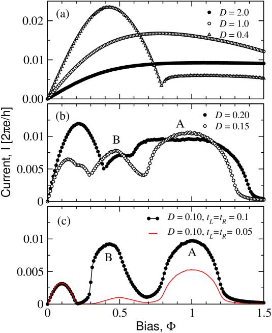
Figure 3: $I-V$ characteristics for narrow bandwidth limit. $t_{L}=t_{R}=0.1$ (except for (c)), $\omega_{ph}=1$, $g=0.2$ and $T=1/12=0.0833$. (a) The saturated current in the large bandwidth limit gradually turns into negative differential resistance regime as $\Phi$ becomes comparable to $D$. (b) Three-peak structure emerges as $D$ gets further reduced. The peaks correspond to ballistic coherent transport, phonon-assisted tunneling (B, $\Phi=\omega_{ph}$) and sequential off-resonant transport (A, $\Phi=2\omega_{ph}$). (c) Reduction of tunneling parameter $t_{L},t_{R}$ dramatically suppresses the phonon-assisted tunneling compared to the sequential current.

In the narrow band limit, one obtains a negative differential resistance (NDR) behavior tsui . FIG. 3 shows the results when the bandwidth $D$ is gradually decreased. Parameters are $\omega_{ph}=0.5,\,t_{L}=t_{R}=0.1$ (except in (c) as shown) and $T=1/12=0.0833$. As $D$ becomes comparable to $\Phi$, a gradual NDR shows up due to the decreasing overlap of $L-R$ DOS. As $D$ is further decreased a distinct discrete three-peak feature emerges as shown in FIG. 3(b-c). The peak at near the zero bias is the coherent current corresponding to the ballistic transport renormalized by the interaction. As $D$ is reduced well below $T$, the maximum height of the ballistic current gets reduced due to the thermal dephasing.

The phonon satellite peak at higher bias ($\Phi=2\omega_{ph}=1$, marked as A in the plot) becomes evident in FIG. 3(b). The electronic transport in this regime is sequential datta_book , i.e., electron from the $L$-reservoir tunnels to the QD by emitting a phonon and loses its phase information before it tunnels out to the $R$-reservoir after emitting another phonon. The width of the structure is twice as large as the full bandwidth, $4D$, as expected. It is interesting that the phonon structures for $D=0.20$ have the familiar stair-case $I-V$ curve, which shows that the phonon satellite states act like discrete current channels due to the reduced decay paths to continuum, in contrast to the large bandwidth limit where the phonon acts more as a dephaser than as a discrete level. We emphasize that the phonon satellite features $A$ and $B$ are due to the first order correction to $\hat{Y}$, particularly the $p$-term in $\hat{Y}_{1}$.

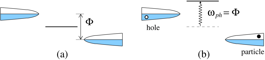
Figure 4: (a) Initial and (b) final states in the phonon assisted tunneling process. The particle-hole and phonon excitations are resonant at the bias $\Phi=\omega_{ph}$.

An intriguing feature in the $I-V$ curves is the phonon-assisted tunneling marked as $B$ in FIG. 3. As depicted in FIG. 4, the tunneling happens by energy-exchange between a particle-hole pair across the device and a phonon on the QD at the bias $\Phi=\omega_{ph}$. The curves at $D=0.4,0.2$ resemble the experimental results tsui . This is a direct consequence of the coherence built in the $\hat{Y}$ operator, Eq. (9), and should be distinguished from the sequential tunneling. To demonstrate the point, a calculation with reduced tunneling parameters $t_{L}=t_{R}=0.05$ is shown as a thin line in FIG. 3(c). Since the phonon-assisted tunneling is through a coherent electron-hole state, the tunneling amplitude is proportional to its cross-lead overlap $t_{L}t_{R}$, while the amplitude of the sequential tunneling is proportional to $t_{L}$ or $t_{R}$ separately due to the uncorrelated sequential tunneling events. The much reduced peak $B$ supports the argument.

We have formulated a quantum simulation algorithm for steady-state nonequilibrium and have shown that the method reproduced the most important physics in the electron-phonon coupled quantum dot system. In combination with other numerical manybody techniques, the formulation of nonequilibrium shown here will provide a critical step toward a more complete theory of steady-state nonequilibrium.

- (1) S. Datta, Electronic Transport in Mesoscopic Systems, Cambridge University Press, Cambridge UK (1995).
- (2) J. Rammer and H. Smith, Rev. Mod. Phys. 58, 323 (1986).
- (3) N. S. Wingreen, K. W. Jacobsen, and J. W. Wilkins, Phys. Rev. Lett. 61, 1396 (1988); N. S. Wingreen, K. W. Jacobsen, and J. W. Wilkins, Phys. Rev. B 40, 11834 (1989).
- (4) R. Lake and S. Datta, Phys. Rev. B 45, 6670 (1992).
- (5) R. Blankenbecler, D. J. Scalapino, and R. L. Sugar, Phys. Rev. D 24, 2278 (1981).
- (6) S. Hershfield, Phy. Rev. Lett. 70, 2134 (1993).
- (7) In the narrow band limit, there are localized states which cannot be included in . However they do not contribute to .
- (8) A. Schiller and S. Hershfield, Phys. Rev. B 51, 12896 (1995).
- (9) P. Bokes and R. W. Godby, Phys. Rev. B 68, 125414 (2003).
- (10) R. M. Fye and J. E. Hirsch, Phys. Rev. B 38, 433 (1988).
- (11) J. W. Negele and H. Orland, Quantum Many-Particle Systems, Addison-Wesly Publishing Company, New York (1988).
- (12) D. E. Feldman, http://arXiv.org: cond-mat/0501133.
- (13) V. J. Goldman, D. C. Tsui, and J. E. Cunningham, Phys. Rev. Lett. 58, 1256 (1987).
- (14) This expression does not include summation over spins.
- (15) M. Jarrell and J. E. Gubernatis, Phys. Rep. 269, 2278 (1981).
- (16) Direct analytic continuation at finite bias does not have an obvious physical meaning since the Green functions (see Eq. (11)) have poles from , not .