Time Resolved Correlation measurements of temporally heterogeneous dynamics

Abstract

Time Resolved Correlation (TRC) is a recently introduced light scattering technique that allows to detect and quantify dynamic heterogeneities. The technique is based on the analysis of the temporal evolution of the speckle pattern generated by the light scattered by a sample, which is quantified by $c_{I}(t,\tau)$, the degree of correlation between speckle images recorded at time $t$ and $t+\tau$. Heterogeneous dynamics results in significant fluctuations of $c_{I}(t,\tau)$ with time $t$. We describe how to optimize TRC measurements and how to detect and avoid possible artifacts. The statistical properties of the fluctuations of $c_{I}$ are analyzed by studying their variance, probability distribution function, and time autocorrelation function. We show that these quantities are affected by a noise contribution due to the finite number $N$ of detected speckles. We propose and demonstrate a method to correct for the noise contribution, based on a $N\rightarrow\infty$ extrapolation scheme. Examples from both homogeneous and heterogeneous dynamics are provided. Connections with recent numerical and analytical works on heterogeneous glassy dynamics are briefly discussed.

I Introduction

Soft glassy systems such as concentrated colloidal suspensions, emulsions, surfactant phases, gels and foams exhibit very slow and unusual dynamics, characterized by non-exponential relaxations of correlation and response functions, which often depend on sample history and may be heterogeneous both in space and time Cipelletti and Ramos (2005). These phenomena have attracted a great interest, in part due to their “universal” character. Examples of unifying descriptions are the mode coupling theory of the stationary average dynamics of concentrated suspensions of particles with both repulsive or attractive interactions Dawson et al. (2001); Eckert and Bartsch (2002); Pham et al. (2002) or, at a more qualitative level, the concept of jamming, which rationalizes the fluid-to-solid transition in a wide range of systems and experimental configurations Liu and Nagel (1998). Additionally, soft glassy materials often exhibit intriguing similarities with hard condensed matter glasses, such as the dependence of the dynamics on sample history (aging phenomena Cipelletti et al. (2000); Knaebel et al. (2000), rejuvenation and memory effects Viasnoff and Lequeux (2002); Bonn et al. (2002)) or the presence of dynamical heterogeneity (Weeks et al. (2000); Kegel and van Blaaderen (2000); Mayer et al. (2004)).

Light scattering is a popular means to measure the average dynamics. In a traditional dynamic light scattering experiment, one measures the normalized time autocorrelation function of the scattered intensity: $\overline{g_{2}(\tau)}=\overline{I_{1}(t)I_{1}(t+\tau)}/\overline{I_{1}(t)}^{2}$, where the average $\overline{\cdot\cdot\cdot}$ is over time, $t$, and $I_{1}(t)$ is the intensity collected by a single detector. The intensity autocorrelation function provides quantitative information on the dynamics of the sample; the way this information is extracted depends on the experimental configuration. In single scattering experiments, $\overline{g_{2}(\tau)}$ is related to the intermediate scattering function, $f(\tau)$, via the Siegert relation: $f(\tau)=\sqrt{\beta^{-1}\left(\overline{g_{2}(\tau)}-1\right)}$, where $\beta$ is the coherence factor that depends on the size ratio between the speckle —or coherence area— and the detector  Berne and Pecora (1976); Goodman (1975). In the opposite limit of strong multiple scattering, the diffusing-wave spectroscopy (DWS) formalism  Weitz and Pine (1993) allows the particle mean square displacement to be calculated from $\overline{g_{2}(\tau)}-1$, provided that the dynamics be spatially and temporally homogeneous. For glassy systems the average over time required to compute $\overline{g_{2}(\tau)}$ may become in practice unfeasible, either because the dynamics is so slow that prohibitively long experiments would be required to accumulate a satisfactory statistics, or because the dynamics may be non-stationary, e.g. for aging systems. Various schemes have been introduced to address this issue, most of them based on the idea of measuring $g_{2}(\tau)$ for many independent speckles and averaging the intensity correlation function not only over time, but also over distinct speckles. This can be done either sequentially –e.g. by slowly rotating the sample so as to illuminate a single detector with different speckles (interleave Muller and Palberg (1996) or echo Pham et al. (2004) methods)– or in parallel, e.g. by using the pixels of a charge-coupled device camera (CCD) as independent detectors (multispeckle method Wong and Wiltzius (1993); Kirsch et al. (1996); Cipelletti and Weitz (1999)).

These techniques drastically reduce the required time average and thus extend the applicability of light scattering to glassy systems. Similarly to traditional light scattering measurements, however, they provide information only on the average dynamics, not on its fluctuations. However, recent theoretical and simulation works suggest that dynamic heterogeneity is a key feature of the slow dynamics in glassy systems. In view of the very limited number of experiments that directly test this behavior on soft glasses Weeks et al. (2000); Kegel and van Blaaderen (2000), new experimental tools that access fluctuations of the dynamics are needed. We have recently introduced the Time Resolved Correlation (TRC) scheme Cipelletti et al. (2003), a method that allows temporally heterogeneous dynamics to be investigated by scattering techniques. The idea at the heart of TRC is that the temporal evolution of the speckle pattern generated by the scattered light will be very different for homogeneous $vs.$ heterogeneous dynamics. For homogeneous dynamics, we expect the speckle images to change smoothly in time. By contrast, for heterogeneous dynamics the speckle pattern is expected to evolve discontinuously, because the rate of change of the sample configuration will not be constant but rather fluctuate with time. Experimentally, the speckle images are recorded by a CCD camera and their evolution is quantified by introducing $c_{I}(t,\tau)$, the degree of correlation between images taken at time $t$ and $t+\tau$ (a rigorous definition will be given in sec. II). Inspection of the $t$-dependence of $c_{I}$ at fixed $\tau$ allows temporally heterogeneous dynamics to be discriminated from homogeneous dynamics. Indeed, in the former case a large drop (increase) of $c_{I}$ is observed whenever the dynamics is faster (slower) than average, while in the latter the degree of correlation is constant. This method is quite general, since it can be applied to any experimental configuration where a multi-element detector can be used to record the speckle pattern generated by a sample illuminated by coherent radiation. Examples are CCD-based light scattering experiments in the single scattering regime, both at wide Kirsch et al. (1996) and small angle Cipelletti and Weitz (1999), DWS in the transmission Viasnoff et al. (2002) or backscattering Cardinaux et al. (2002) geometry, and X-photon Correlation Spectroscopy (XPCS) at small angles Diat et al. (1998). In principle, the technique could also be extended to non-electromagnetic radiation, e.g. to acoustic DWS Cowan et al. (2002).

Experiments on diluted suspensions of colloidal Brownian particles have shown that the degree of correlation exhibits some fluctuations even in the absence of dynamic heterogeneity Cipelletti et al. (2003). As it will be shown in detail, these fluctuations are due to statistical noise stemming from the finite number of speckles in the CCD images. In order to exploit quantitatively TRC data it is thus necessary to separate the contribution to the fluctuations of $c_{I}$ due to the noise from that due to dynamic heterogeneity. Although in most cases it is not possible to directly correct the TRC time series for the noise, we will show that it is possible to correct statistical quantities derived from the TRC data and used to quantify the fluctuations of $c_{I}$. We focus in particular on three statistical objects: the time variance of $c_{I}(t,\tau)$, the probability distribution function (PDF) of $c_{I}(t,\tau)$ for a fixed $\tau$, and the time autocorrelation of the $c_{I}(t,\tau)$ trace itself.

The variance of $c_{I}$, $\sigma^{2}_{c_{I}}(\tau)$, is the lowest moment of the data that provides information on the fluctuations. It corresponds to the so-called dynamical susceptibility $\chi_{4}$ studied in many simulation and theoretical works on glassy systems Lacevic et al. (2003); Whitelam et al. (2005); Pitard (2005); de Candia et al. (2005). In a typical simulation, $\chi_{4}$ is the variance of the intermediate scattering function, or a similar correlation function describing the system’s change in configuration, which is obtained from several independent runs. Similarly, $\sigma^{2}_{c_{I}}$ quantifies the fluctuations of the intensity correlation function as the system evolves through statistically independent configurations. Importantly, $\sigma^{2}_{c_{I}}$ allows one to relate temporal dynamic heterogeneity to spatial correlations of the dynamics. In fact, it can be shown that $\chi_{4}$ is the volume integral of the spatial correlation of the local dynamics Lacevic et al. (2002). Therefore, large values of $\sigma^{2}_{c_{I}}$ will be indicative of long-range correlations of the dynamics. Intuitively, one can expect the variance of the fluctuations of the dynamics to scale as the inverse number of “dynamically independent” regions in the scattering volume, and thus to increase as the spatial range of the correlation of the dynamics increases. Recent TRC experiments on a shaving cream foam support this simple picture Mayer et al. (2004).

The PDF of the TRC signal is the most complete statistical characterization of the dispersion of the data. Any deviation from a Gaussian shape immediately hints to heterogeneous dynamics, as suggested by experiments on a variety of systems, including colloidal gels Cipelletti et al. (2003); Bissig et al. (2003a); Sarcia and Hebraud (2005), concentrated colloidal suspensions Ballesta et al. (2004) and surfactant phases Duri et al. (2005), foams Bissig (2004), and granular materials Caballero et al. (2004). Remarkably, the shape of the PDF of $c_{I}$ is often strongly reminiscent of that obtained for similar quantities in theoretical and simulation work on other glassy systems. An example is provided by simulations of spin glasses, where the fluctuations of the correlation function of the spin orientation are distributed according to a generalized Gumbel PDF Chamon et al. (2004), a probability distribution characterized by an exponential tail strikingly similar to those reported for $c_{I}$ in refs. Cipelletti et al. (2003); Bissig et al. (2003a); Sarcia and Hebraud (2005); Ballesta et al. (2004); Duri et al. (2005); Caballero et al. (2004) or shown in this paper (see figs. 8 and 11). Similar distributions are also obtained in a variety of numerical and analytical investigations of systems with heterogeneous dynamics, both at equilibrium and out-of-equilibrium Clusel et al. (2004); Merolle et al. (2005); Crisanti and Ritort (2004); Pitard (2005). Indeed, it has been proposed that the Gumbel distribution arises as a universal PDF for various quantities measured in systems with extended spatial and/or temporal correlations Bramwell et al. (2000). Clearly, in order to compare in detail and quantitatively the PDF measured in TRC experiments to those obtained analytically or by simulations it is necessary to correct the experimental data for the contribution of the measurement noise.

The variance and the PDF of $c_{I}$ describe the dispersion of the data, but are insensitive to the way the fluctuations are distributed in time. By contrast, the time autocorrelation of the TRC signal, which was introduced in ref. Duri et al. (2005) and which we shall term “second correlation”, provides information on the temporal organization of the fluctuations of the dynamics, and sheds light on the rate and life time of rearrangement events. The second correlation introduced here is similar to the 4-th order intensity correlation function proposed by Lemieux and Durian Lemieux and Durian (1999, 2001) and to the multi-time correlation functions measured in nuclear magnetic resonance experiments probing dynamical heterogeneity near the glass transition Schmidtrohr and Spiess (1991). Moreover, we note that the second correlation is the analogous, in the time domain, of the so-called second spectrum originally introduced to investigate non-gaussian fluctuations in the dynamics of spin glasses Weissman (1993).

In this paper, we first describe how to optimize a TRC measurement by correcting the CCD data for the dark noise, due to the electronic noise of the CCD, and for the uneven illumination of the detector (sec. II). We then turn to the temporal fluctuations of $c_{I}$ and analyze separately the contribution of the measurement noise, due to the finite number of pixels, (sec. III) and that due to heterogeneous dynamics (sec. IV). We illustrate our analysis by showing TRC data obtained mainly from a dilute suspension of Brownian particles and a shaving cream foam, two model systems that exhibit homogeneous and heterogeneous dynamics, respectively. We then introduce a method for correcting the experimentally measured variance and PDF of $c_{I}$ for the noise contribution. The method consist of an extrapolation scheme based on the observation that the measurement noise vanishes in the limit $N\rightarrow\infty$ ($N$ being the number of CCD pixels used to calculate $c_{I}$), whereas the fluctuations due to dynamical heterogeneities are independent of $N$. In sec. V we introduce the second correlation and provide a working formula for correcting it for the noise contribution. Possible artifacts that may affect the fluctuations of $c_{I}$ and lead to spurious contributions to its PDF and to the second correlation are discussed in sec. VI, together with methods to detect or correct them. In the concluding section, we briefly discuss the connections between TRC and other techniques that measure dynamical heterogeneities in soft glassy systems, focussing on the advantages and the limitations of the various methods.

II Time Resolved Correlation: measuring the time-dependent degree of correlation $c_{I}(t,\tau)$

In a TRC experiment Cipelletti et al. (2003) a CCD camera is used to record, at constant rate, the speckle pattern of the light scattered by the sample Goodman (1975). The CCD images are stored on the hard disk of a personal computer (PC) for later processing. The degree of correlation, $c_{I}$, between speckle patterns at times $t$ and $t+\tau$ is then calculated according to

$$c_{I}(t,\tau)=\frac{G_{2}(t,\tau)}{I(t)I(t+\tau)}-1~{},$$ (1)

where $G_{2}(t,\tau)=\langle I_{p}(t)I_{p}(t+\tau)\rangle_{p}$ and $I(t)=\langle I_{p}(t)\rangle_{p}$, with $I_{p}(t)$ the intensity measured at time $t$ by the $p$-th CCD pixel and $\langle\cdot\cdot\cdot\rangle_{p}$ an average over $N$ pixels. Note that the normalization factor in Eq. (1), $I(t)I(t+\tau)$, allows to cancel out exactly any fluctuations due to changes in the laser power. For stationary dynamics, the intensity correlation function usually measured in a light scattering experiment, $\overline{g_{2}(\tau)}$, may be obtained from $\overline{g_{2}(\tau)}-1=\overline{c_{I}(t,\tau)}$.

In Eq. (1) the intensity value at each pixel is required. In practice, however, the images recorded by the CCD are affected by a pixel- and time-dependent dark (or electronic) noise, $D_{p}(t)$, and, possibly, by the non-uniform illumination of the detector, depending on the setup optics. To account for these effects, we write the raw signal for pixel $p$, $S_{p}$, as $S_{p}(t)=I_{p}(t)b_{p}/\langle b_{p}\rangle_{p}+D_{p}(t)$, where $b_{p}$ is a time-independent, spatially slowly-varying function that accounts for non-uniform illumination and $\langle b_{p}\rangle_{p}$ is introduced so that the factor multiplying $I_{p}(t)$ has unit average. Prior to each measurement, we collect 100 dark images by covering the CCD detector with a black cap. These dark images are used to calculate the time-averaged dark noise $\overline{D_{p}}$. The raw signal is corrected by subtracting, pixel-by-pixel, the average dark noise. To estimate $b_{p}$, we average over time the dark-noise-corrected CCD signal : $b_{p}=\overline{S_{p}(t)}-\overline{D_{p}}$. For experiments whose duration, $T_{\rm exp}$, is much longer than the relaxation time of $\overline{g_{2}(\tau)}$, $\tau_{0}$, this procedure averages out the spatial fluctuations associated with the speckles and leads to a smooth function $b_{p}$, since for each pixel the intensity fully fluctuates many times and its time average is a good estimator of the mean intensity at a given location of the CCD detector. By contrast, when $T_{\rm exp}\lesssim\tau_{0}$, $b_{p}$ keeps some memory of the speckled appearance of the instantaneous intensity distribution. In this case, we further smooth $b_{p}$ by averaging it over a few adjacent pixels. The desired intensity to be used in Eq. (1) is obtained from

$$I_{p}(t)=[S_{p}(t)-\overline{D_{p}}]\langle b_{p}\rangle_{p}/b_{p}.$$ (2)

Note that $I_{p}(t)$ is still affected by an instanteneous noise $\epsilon_{p}(t)=D_{p}(t)-\overline{D_{p}}$, since only the average dark noise could be subtracted. By definition, $\overline{\epsilon_{p}}=0$, while the standard deviation $\sigma_{\epsilon}$ of $\epsilon$ is typically of the order of 1/100 of the saturation level for an 8-bit CCD camera. When all the relevant time scales of the dynamics are much longer than the inverse CCD rate, $\epsilon_{p}(t)$ may be considerably reduced by averaging $I_{p}(t)$ over a few CCD images before applying Eq. (1). In the following, we will disregard $\epsilon_{p}(t)$, unless when explicitly stated.

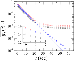
Figure 1: Semi-logarithmic plot of the intensity time autocorrelation function measured for a suspension of monodisperse Brownian particles in the single scattering regime ($\theta=45$ deg). Data are averaged over $N$ = 151800 pixels and over $T_{\rm exp}=10800$ sec. Squares: intensity autocorrelation function calculated from the CCD raw signal, $S_{p}(t)$; circles: the same data after correcting for the dark noise only; triangles: after correcting for both the dark noise and the uneven detector illumination. The line is a fit to the corrected data by a single exponential decay, the functional form of $\overline{g_{2}}-1$ predicted for monodisperse Brownian particles, yielding a characteristic time $\tau_{0}=5.8$ sec. Inset: zoom of the small $\tau$ behavior of the intensity autocorrelation function.

We show in fig. 1 how the different corrections discussed above affect the intensity autocorrelation function measured for a dilute suspension of monodisperse Brownian particles. Data are collected in the single scattering geometry, at a scattering angle $\theta=45$ deg. The particles are polystyrene spheres of radius $a=265$ nm, suspended at a volume fraction $\phi=3.7\times 10^{-5}$ in almost pure glycerine cooled at 15 ${}^{\rm o}\rm{C}$ in order to make the dynamics slow enough to match the limited acquisition rate of the CCD, which is 2 Hz in this experiment. Both the dark noise and the non-uniform illumination result in a spurious increase of the base line of the autocorrelation function (squares and circles in fig. 1) and lead to a change of its $\tau\rightarrow 0$ intercept (see inset). However, the relaxation time obtained from the small $\tau$ behavior of the intensity autocorrelation function is essentially unaffected by the dark noise and the non-uniform illumination. When the CCD signal is corrected according to Eq. (2) (up triangles), a single exponential decay is observed, as predicted for monodisperse Brownian particles. For the corrected data, the base line is limited only by the dark noise $\epsilon_{p}(t)$: its value is of the order of $2\times 10^{-4}$ and is comparable to that obtained in traditional light scattering setups, which use a photomultiplier tube or an avalanche photodiode as a detector.

III Temporal fluctuations of $c_{I}(t,\tau)$: the noise contribution

When disregarding the fluctuations of $\epsilon_{p}(t)$, the temporal fluctuations of the degree of correlation $c_{I}(t,\tau)$ at a fixed lag $\tau$ have only two independent sources: the statistical noise due to the finite number of speckles probed in the experiment and the intrinsic fluctuations of the sample dynamics. The first contribution is always present: we shall refer to it as to the “measurement noise”, not to be confused with the dark noise discussed in Sec. II. The second contribution, on the contrary, is present only if the dynamics is temporally heterogeneous and thus represents the physically valuable information that we aim to extract from the fluctuations of $c_{I}$. To highlight the two different contributions, we rewrite Eq. (1) as

$$c_{I}(t,\tau)=g_{2}(a_{1}(t),...,a_{k}(t);\tau)-1+n(t,\tau),$$ (3)

where $n(t,\tau)$ is the measurement noise, with $\overline{n(t,\tau)}=0$, and $g_{2}(a_{1}(t),...,a_{k}(t);\tau)-1$ is the pixel-averaged two-time intensity correlation function that would be measured in the absence of any noise, i.e. if $c_{I}$ was averaged over an infinite number of speckles. $a_{1}(t),...,a_{k}(t)$ are parameters that fluctuate with time if the dynamics are heterogeneous, but are constant for homogeneous dynamics.

To illustrate this point, let us consider as an example of homogeneous dynamics the single scattering measurement of the dynamics of monodisperse Brownian particles at a scattering vector $q$. If the temperature is carefully controlled, the diffusion coefficient $D$ of the particles does not evolve with time and $g_{2}(a_{1}(t),...,a_{k}(t);\tau)-1=a_{1}\exp(-a_{2}\tau)$, with $a_{1}=\beta$ and $a_{2}=2q^{2}D$ constant Berne and Pecora (1976). In this case, the fluctuations of $c_{I}$ are due only to the noise $n(t,\tau)$. By contrast, the spatially and temporally localized bubble rearrangements in a shaving cream foam provide a simple example of heterogeneous dynamics. For a foam, the average intensity correlation function measured in a DWS experiment in the transmission geometry has a shape very close to that for Brownian particles in single scattering: $\overline{g_{2}}(\tau)-1=\beta\exp[-(2\overline{\gamma}\tau)^{\overline{\mu}}]$, with $\overline{\mu}\approx 0.9$ and $\overline{\gamma}=\overline{R}r^{3}L^{2}/l^{*2}$ Durian et al. (1991) . Here, $\overline{R}$ is the average bubble rearrangement rate per unit time and unit volume, $r^{3}$ is the typical volume that is rearranged by a single event, $L$ is the sample thickness, and $l^{*}$ is the photon transport mean free path. In contrast with the Brownian suspension, however, the degree of correlation measured for a foam fluctuates not only because of the noise, but also because the instantaneous rearrangement rate continuously changes due to the intermittent nature of the bubble dynamics Bissig (2004); Mayer et al. (2004). Hence, for the foam $g_{2}(a_{1}(t),...,a_{k}(t);\tau)-1=a_{1}\exp[-(a_{2}(t)\tau)^{a_{3}(t)}]$, with $a_{1}=\beta$ constant while $a_{2}(t)=R(t)r^{3}L^{2}/l^{*2}$ and $a_{3}(t)=\mu(t)$ fluctuate with time.

In view of the correction scheme described in secs. IV and V, it is useful to first analyze the contribution to the fluctuations of $c_{I}$ due to the noise. We assume that the sample dynamics be temporally homogeneous and stationary, as for the dilute suspension of Brownian particles discussed above. In this case, the parameters $a_{1},...,a_{k}$ in Eq. (3) are constant and the fluctuations of $c_{I}$ are due only to the noise term, $n(t,\tau)$. Since $c_{I}(t,\tau)$ is averaged over a large number of pixels (typically $N\gtrsim 10000$), its temporal fluctuations at a fixed $\tau$ are expected to be Gaussian distributed, because of the central limit theorem (see Appendix B). Accordingly, only $\overline{c_{I}}$ and the variance $\sigma^{2}_{n}(\tau)$ of the noise $n(t,\tau)$ are needed to obtain the full probability distribution of $c_{I}$: $P_{c_{I}}(c_{I})=(2\pi\sigma^{2}_{n})^{-1/2}\exp[-(c_{I}-\overline{c_{I}})^{2}/2\sigma^{2}_{n}]$. For homogeneous dynamics, $\sigma^{2}_{n}(\tau)=\sigma^{2}_{c_{I}}(\tau)\equiv\overline{c_{I}(t,\tau)^{2}}-\overline{c_{I}(t,\tau)}^{2}$. To calculate $\sigma^{2}_{c_{I}}$, we recall that the variance of a quantity $y$ that depends on the $m$ variables $x_{1},...,x_{m}$ is given by

$$\sigma^{2}_{y}=\sum_{i=1}^{m}\left[\frac{\partial y}{\partial x_{i}}\right]_{x_{i}=\overline{x_{i}}}^{2}\sigma_{x_{i}}^{2}+\sum_{i\neq j}\left[\frac{\partial y}{\partial x_{i}}\frac{\partial y}{\partial x_{j}}\right]_{x_{i}=\overline{x_{i}}\atop x_{j}=\overline{x_{j}}}\sigma_{x_{i},x_{j}},$$ (4)

where $\sigma^{2}_{x_{i}}\equiv\overline{x_{i}^{2}}-\overline{x_{i}}^{\,2}$ is the variance of $x_{i}$ and $\sigma_{x_{i},x_{j}}\equiv\overline{x_{i}x_{j}}-\overline{x_{i}}\,\overline{x_{j}}$ is the covariance between $x_{i}$ and $x_{j}$ ($i\neq j$). The first sum accounts for the sensitivity of $y$ to the fluctuations of the independent variables $x_{1},...,x_{m}$, while the second sum accounts for any correlations between the $x_{i}$’s. If distinct $x_{i}$’s are uncorrelated, $\overline{x_{i}x_{j}}=\overline{x_{i}}\,\overline{x_{j}}$ for $i\neq j$ and the second sum vanishes.

By applying Eq. (4) to the definition of $c_{I}$, Eq. (1), we find

$$\sigma^{2}_{c_{I}}(\tau)=1/\overline{I}^{4}\sigma^{2}_{G_{2}}(\tau)+2\overline{G_{2}(\tau)}^{2}/\overline{I}^{6}\sigma^{2}_{I}$$

$${}+2\overline{G_{2}(\tau)}^{2}/\overline{I}^{6}\sigma_{I,J}(\tau)-4\overline{G_{2}(\tau)}/\overline{I}^{5}\sigma_{G_{2},I}(\tau),$$ (5)

where we have introduced the notation $J(t)\equiv I(t+\tau)$. In writing Eq. (5), we have used $\overline{I}=\overline{J}$ and $\sigma_{G_{2},I}=\sigma_{G_{2},J}$, because the scattered light was assumed to be stationary.

The physical origin of the fluctuations of $I$ and $G_{2}$, quantified by $\sigma^{2}_{I}$ and $\sigma^{2}_{G_{2}}$, as well as that of the correlation between $I$ and $J$ and between $I$ and $G_{2}$, quantified by $\sigma_{I,J}$ and $\sigma_{G_{2},I}$, is the finite number of pixels over which the instantaneous intensity and the intensity correlation are averaged. To illustrate this point, let us consider as an example $I(t)$. As the sample evolves through different configurations, the speckle pattern fluctuates with a characteristic time $\tau_{0}$. Since the instantaneous pixel-averaged intensity is calculated for a finite set of speckles, different speckle patterns yield slightly different values of $I(t)$. The larger the number of the sampled speckles, the closer will $I(t)$ be to the “true” value of the average scattered intensity, whose estimator is $\overline{I}$, and thus the smaller will be $\sigma^{2}_{I}$. Indeed, we show in Appendix A that $\sigma^{2}_{I}\sim N^{-1}$, as expected from the central limit theorem . Moreover, one expects the instantaneous pixel-averaged intensity at time $t$ to be correlated to the same quantity measured at time $t+\tau$, at least for $\tau\lesssim\tau_{0}$, because it takes a few $\tau_{0}$ for the speckle pattern to be completely renewed. Therefore, the covariance term $\sigma_{I,J}(\tau)$ will vanish only for $\tau\gg\tau_{0}$. More precisely, we expect $\sigma_{I,J}(\tau)$ to be proportional to $\overline{G_{2}(\tau)}$. In fact, $\sigma_{I,J}(\tau)$ is precisely the un-normalized correlation function measured by using the whole CCD chip as a single detector, similarly to the case of a traditional light scattering experiment where the detector collects a large number of speckles.

Similar arguments may be invoked for $\sigma^{2}_{G_{2}}(\tau)$ and $\sigma_{G_{2},I}(\tau)$, suggesting that the variance and covariance factors in Eq. (5) scale with $N^{-1}$ and depend linearly on the average correlation function:

$$\sigma_{x_{i},x_{j}}(\tau)=N^{-1}[A_{x_{i},x_{j}}+B_{x_{i},x_{j}}\overline{c_{I}(\tau)}],$$ (6)

where $x_{i}$ and $x_{j}$ stand for any of $I$, $J$, and $G_{2}$, while $A_{x_{i},x_{j}}$ and $B_{x_{i},x_{j}}$ are constants whose values are given in Appendix A. To test the linear dependence of the variance and covariance factors on the time-averaged correlation function, we plot parametrically $\sigma^{2}_{G_{2}}(\tau)$, $\sigma_{I,J}(\tau)$, and $\sigma_{G_{2},I}(\tau)$ as a function of $\overline{c_{I}}(\tau)$, for data obtained in the single scattering experiment on Brownian particles, as shown in fig. 2. In all cases the data are very well fitted by straight lines, thus confirming the validity of Eq. (6).

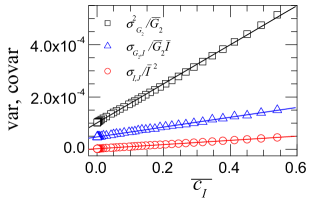
Figure 2: Parametric plot of the normalized variance and covariance terms in the r.h.s. of Eq. (5), as a function of $\overline{c_{I}(\tau)}$, for the same experiment as in fig. 1. The lines are linear fits to the data, suggesting the $c_{I}$ dependence of Eq. (6).

The $\tau$ dependence of the variance of the measurement noise can be obtained by substituting Eq. (6) into Eq. (5). Using $\overline{G_{2}(\tau)}=\overline{I}^{2}(\overline{c_{I}(\tau)}+1)$ (see Appendix B), one finds a third order polynomial dependence of the variance of $n(t,\tau)$ on $\overline{c_{I}(\tau)}$:

$$\sigma^{2}_{n}(\tau)=\sigma^{2}_{c_{I}}(\tau)=N^{-1}\sum_{l=0}^{3}\alpha_{l}\overline{c_{I}(\tau)}^{\,l},$$ (7)

where the coefficients $\alpha_{l}$ can be obtained from $\overline{I}$, $A_{x_{i},x_{j}}$, and $B_{x_{i},x_{j}}$. Note that this third-order polynomial dependence is due to the choice of the normalization of $c_{I}$ (see Eq. (1)). If the denominator was chosen to be $\overline{I}^{2}$, as in traditional light scattering experiments, only the first term in the r.h.s. of Eq. (5) would be non-zero and $\sigma^{2}_{c_{I}}(\tau)\propto\sigma^{2}_{G_{2}}$, i.e. the fluctuations would increase linearly with $\overline{c_{I}(\tau)}$. Although the normalization we have chosen leads to a more complicated expression for $\sigma^{2}_{n}(\tau)$, we remind that it suppresses spurious variations of $c_{I}$ due to fluctuations of the incoming beam power and thus should be used in TRC experiments. The inset of fig. 3 shows a semi-logarithmic plot of $\sigma_{c_{I}}(\tau)$ $vs.$ $\tau$ for the Brownian particles, confirming that the noise of $c_{I}$ decreases with $\tau$, as indicated by Eq. (7). In the main plot, the same data are plotted parametrically as a function of $\overline{c_{I}}(\tau)$. A very good agreement is found between the experimental data and the polynomial form suggested by Eq. (7), as shown by the line.

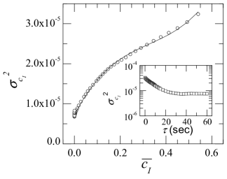
Figure 3: Main plot: parametric representation of the variance of $c_{I}$ as a function of $\overline{c_{I}(\tau)}$ for the same experiment as in figs. 1 and 2 (single scattering from a dilute suspension of Brownian particles). The line is a fit of Eq. (7) to the data. Inset: same data plotted $vs.$ $\tau$.

The $N^{-1}$ dependence of $\sigma_{n}^{2}(\tau)$ is the key feature that will be exploited in the correction for the measurement noise. To test this scaling, we analyze the time series of speckle images recorded for the Brownian particle suspension, for which $\sigma^{2}_{c_{I}}=\sigma^{2}_{n}$, by processing different number of pixels. First, all pixels of each image are processed and $c_{I}(t,\tau)$ and its variance $\sigma^{2}_{c_{I}}(\tau)$ are calculated. Each image is then divided into two regions of interest (ROI) of equal size. For each ROI, $c_{I}$ and its variance are calculated and the values of $\sigma^{2}_{c_{I}}(\tau)$ obtained for the two ROIs are averaged, yielding the variance of $c_{I}$ when only $N/2$ pixels are processed. This scheme is iterated until the size of each ROI is reduced to 225 pixels. Figure 4 shows $\sigma^{2}_{c_{I}}(\tau)$ as a function of the inverse number of processed pixels, $N^{-1}$, for three time delays corresponding to 0.09, 0.87, and 8.7 times the relaxation time of $\overline{g_{2}}-1$, respectively. In all cases, the data for $N^{-1}<1.2\times 10^{-4}$ are very well fitted by a straight line that goes through the origin, as shown in the inset . This confirms that for temporally homogeneous dynamics $\sigma^{2}_{c_{I}}\propto N^{-1}$, as indicated by Eq. (7). Note that a deviation from this linear trend is observed at the largest $N^{-1}$, due to edge effects. In fact, the contribution of each pixel to $c_{I}$ is not completely independent from that of nearby pixels, because the intensity of the speckle pattern is spatially correlated over a distance of a few pixels. Pixels far from the edges of a ROI have more nearby pixels than those on the edges; accordingly, the statistically independent contribution to $c_{I}$ carried by a bulk pixel is less than that of an edge pixel. When reducing the size of the processed ROI, the weight of edge pixels relative to bulk pixels increases and corrections to the $N^{-1}$ scaling become increasingly apparent. These corrections are negligible for $N\gtrsim 8000$, as seen in fig. 4. We find that a similar $N^{-1}$ scaling is obtained at all time delays (data not shown). Indeed, the slopes of the straight line fits to $\sigma^{2}_{c_{I}}$ $vs.$ $N^{-1}$ provide an estimate of the proportionality coefficient $\sum_{l=0}^{3}\alpha_{l}\overline{c_{I}(\tau)}^{l}$ that agrees within $1\%$ with the value directly obtained when calculating $\sigma^{2}_{c_{I}}$ by processing the maximum number of available pixels.

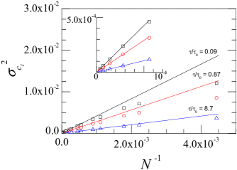
Figure 4: For the same experiment on Brownian particles as in the preceding figures: variance of $c_{I}$ as a function of the inverse number of pixels over which $c_{I}$ is averaged. The lines are linear fits to the data for $N^{-1}\leq 1.2\times 10^{-4}$, demonstrating that for large $N$ $\sigma^{2}_{c_{I}}\propto N^{-1}$. The inset zooms in the region near to the origin.

For temporally homogeneous dynamics, the statistics of the variables $G_{2}(t,\tau)$ and $I(t)$ in Eq. (1) is Gaussian, because of the central limit theorem. As a consequence, the probability density function (PDF) of $c_{I}$ is also Gaussian, as demonstrated in Appendix B. In fig. 5 we show the PDF of $c_{I}$ for various $\tau$ for a Brownian suspension of particles. The symbols are the experimental data, while the lines are Gaussian PDFs with mean $\overline{c_{I}(\tau)}$ and standard deviation $\sigma_{c_{I}}(\tau)$ obtained directly from the $c_{I}$ time series, without any fitting parameters. An excellent agreement between the data and the theoretical shape of the distributions is observed at all $\tau$.

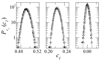
Figure 5: Symbols: PDF of $c_{I}(t,\tau)$, $P_{c_{I}}(c_{I})$, for the same suspension of Brownian particles as for the preceding figures. From left to right, the normalized delay $\tau/\tau_{0}$ is 0.09, 0.87, and 8.7. In the three panels the $c_{I}$ axis spans an interval of equal width (0.04). The lines are Gaussian distributions whose mean and standard deviations are directly obtained from the $c_{I}$ time series, without any fitting parameter.

IV Temporally heterogeneous dynamics: corrections for the noise contribution

In temporally heterogeneous dynamics, the fluctuations of $c_{I}$ are due both to the noise and to dynamical heterogeneity. In this section we propose a method for correcting the variance and the PDF of $c_{I}$ for the noise contribution, so as to obtain the statistics of the fluctuations due to dynamical heterogeneity. Moreover, we show that in some instances the full temporal evolution of $c_{I}$ may be corrected for the noise, thus allowing $g_{2}(t,\tau)-1$ to be determined, not only its variance and PDF.

IV.1 Correction of the variance of $c_{I}$

In the case of dynamically heterogeneous processes, the parameters $a_{1},...,a_{k}$ in the two-time correlation function $g_{2}(a_{1}(t),...,a_{k}(t);\tau)-1$, Eq. (3), fluctuate with $t$. Therefore, an extra term, $\sigma_{g_{2}}$, contributes to the variance of $c_{I}$, in addition to the noise term analyzed in the preceding section:

$$\sigma^{2}_{c_{I}}(\tau)=N^{-1}\sum_{l=0}^{3}\alpha_{l}\overline{c_{I}(\tau)}^{\,l}+\sigma^{2}_{g_{2}}(\tau).$$ (8)

In writing the expression above, we have assumed that no correlation exists between the noise $n(t,\tau)$ due to the finite number of pixels and the fluctuations of $a_{1},...,a_{k}$. Using Eq. (4), $\sigma_{g_{2}}^{2}$ may be expressed as

$$\sigma^{2}_{g_{2}}(\tau) = \sum_{i=1}^{k}\left[\frac{\partial g_{2}}{\partial a_{i}}\right]_{a_{i}=\overline{a_{i}}}^{2}\sigma_{a_{i}}^{2}$$ (9)

$$+ \sum_{i\neq j}\left[\frac{\partial g_{2}}{\partial a_{i}}\frac{\partial g_{2}}{\partial a_{j}}\right]_{a_{i}=\overline{a_{i}}\atop a_{j}=\overline{a_{j}}}\sigma_{a_{i},a_{j}}.$$

An example where $\sigma^{2}_{g_{2}}$ assumes a particularly simple form is given by the dynamics of a shaving cream foam, resulting from intermittent bubble rearrangements, as measured in a DWS experiment. We find that the fluctuations in the instantaneous decay rate $\gamma(t)$ of the correlation function are slow compared to $\overline{\gamma}$, so that at any given time $g_{2}-1$ is well approximated by a stretched exponential, $\beta\exp[-(\gamma(t)\tau)^{\mu(t)}]$. Small variations of $\mu(t)$ account for slight changes of the decay rate on a time scale comparable to $\overline{\gamma}^{\,-1}$. For example, if the dynamics tend to slow down during the measurement of $g_{2}-1$, the initial decay of the correlation function will be faster than its final decay. Thus, the shape of $g_{2}$ will be more stretched than the average one ($\mu<\overline{\mu})$. Conversely, $\mu>\overline{\mu}$ if the dynamics accelerate during the measurement of $g_{2}-1$. By taking into account the fluctuations of both $\gamma$ and $\mu$, Eq. (9) yields, for the foam,

$$\sigma^{2}_{g_{2}}(\tau) = (\overline{\gamma}\tau)^{2}\beta^{2}\exp\left[-2(\overline{\gamma}\tau)^{\overline{\mu}\,}\right]$$ (10)

$$\times \left\{\left(\frac{\overline{\mu}}{\overline{\gamma}}\sigma_{\gamma}\right)^{2}+\left[\,\ln(\overline{\gamma}\tau)\sigma_{\mu}\right]^{2}\right\}$$

with $\sigma^{2}_{\gamma}=\overline{(\gamma-\overline{\gamma})^{2}}$ and $\sigma^{2}_{\mu}=\overline{(\mu-\overline{\mu})^{2}}$. Equation (10) extends a similar expression given in ref. Mayer et al. (2004), where only the fluctuations of $\gamma$ where taken into account. However, here we still neglect possible correlations between $\gamma$ and $\mu$ that could be described by including the second term of the r.h.s. of Eq. (9).

A direct test of Eq. (10) is not possible, since we experimentally only access $\sigma^{2}_{c_{I}}$, not $\sigma^{2}_{g_{2}}$. Therefore, for the foam as well as for the general case of temporally heterogeneous dynamics it is desirable to subtract the trivial contribution of the measurement noise from the experimentally measured $\sigma^{2}_{c_{I}}$, in order to obtain the physically relevant variance $\sigma^{2}_{g_{2}}$. We have tested two different approaches. In the first method, the linear dependence of $\sigma_{x_{i},x_{j}}$ on $\overline{c_{I}}$ shown in fig. 2 is used to derive formulas for these quantities that are independent of the instantaneous dynamics and thus of the homogeneous $vs.$ heterogeneous nature of the dynamics. These formulas are presented in Appendix A. Unfortunately, although they provide separately fairly good estimates of the various terms $\sigma_{x_{i},x_{j}}$, when combined using eq. 5 to evaluate $\sigma^{2}_{n}$ uncertainties add up leading to errors of the order of $30-40\%$, as tested on the data for the single scattering experiment on the Brownian particles.

In the following, we describe in detail a second method that has proven to be highly effective. The key point is to recognize that, contrary to the noise term, the fluctuations of $g_{2}(a_{1},...,a_{k};\tau)$ do not depend on the number of pixels over which $c_{I}$ is averaged. This is because in the far field geometry of the scattering experiments described in this work, each CCD pixel collects light scattered by the whole illuminated sample. Thus, any spatial or temporal heterogeneity of the dynamics affects in the same way the signal measured by each pixel. The different pixel-number dependence of the noise and the fluctuations (first and second term in the r.h.s. of Eq. (8), respectively) suggests a way to discriminate between these two contributions. We analyze the speckle images by processing different number of pixels, as described for the Brownian suspension in sec. III, and plot $\sigma^{2}_{c_{I}}(\tau)$ as a function of $N^{-1}$, as shown in fig. 6. As indicated by Eq. (8), the slope of a linear fit to the data yields $\sum_{l=0}^{3}\alpha_{l}\overline{c_{I}(\tau)}^{\,l}$, while the intercept at $N^{-1}=0$ is $\sigma_{g_{2}}^{2}(\tau)$, the desired variance of the correlation function due to dynamical heterogeneity. Thus, the representation of figs. 4 and 6 allows one to extrapolate $\sigma_{c_{I}}^{2}$ to $N=\infty$, where the measurement noise vanishes. As seen in the inset of fig. 6, for $\tau\overline{\gamma}\ll 1$ or $\tau\overline{\gamma}\gg 1$ the intercept of the linear fit is very close to zero, indicating that at these delays the fluctuations of $c_{I}$ are mainly determined by the measurement noise. By contrast, at intermediate delays the intercept clearly departs from zero, revealing the intermittent nature of the dynamics of the foam.

In fig. 7 we plot the $\tau$ dependence of $\sigma_{c_{I}}^{2}$ measured for the foam, together with the noise contribution, $\sigma_{n}^{2}=N^{-1}\sum_{l=0}^{3}\alpha_{l}\overline{c_{I}(\tau)}^{\,l}$ , and that of the intrinsic fluctuations, $\sigma_{g_{2}}^{2}$. The noise contribution is extracted from the slope of $\sigma_{c_{I}}^{2}$ $vs.$ $N^{-1}$, while the variance of the intrinsic fluctuations is given by the $N^{-1}\rightarrow 0$ limit of $\sigma_{c_{I}}^{2}$ $vs.$ $N^{-1}$. At all $\tau$ we find $\sigma_{c_{I}}^{2}=\sigma_{n}^{2}+\sigma_{g_{2}}^{2}$ within $0.8\%$, thus confirming that our analysis allows to correctly account for the two contributions to the fluctuations of $c_{I}$. Note that, while the shape of the time-averaged correlation function $\overline{g_{2}}-1$ is almost the same for the foam and the Brownian particles (a slightly stretched exponential for the former and a simple exponential decay for the latter), the $\tau$ dependence of the fluctuations of $c_{I}$ is very different (compare the inset of fig. 3 to fig. 7), thus allowing temporally heterogeneous dynamics to be unambiguously detected. For the foam, correcting $\sigma_{c_{I}}^{2}$ for the noise contribution is especially important at time delays far from the mean relaxation time, because the intrinsic fluctuations die off for $\tau\rightarrow 0$, when virtually no rearrangement had a chance to occur, and for $\tau\rightarrow\infty$, when so many rearrangement events occurred that the statistical fluctuations of their number are negligible. By contrast, we recall that $\sigma_{n}^{2}$ remains finite at all $\tau$. Once corrected for the noise contribution, $\sigma_{g_{2}}^{2}(\tau)$ is very well described by Eq. (10), as shown by the line in fig. 7. Interestingly, the fluctuations are maximal on the time scale of the mean relaxation time, a general feature found also in the dynamic susceptibility $\chi_{4}$ measured in simulations. Intuitively, this can be explained by recognizing that the correlation function is most sensitive to a change of the instantaneous relaxation time for $\tau\approx\tau_{0}$. Finally, note that when comparing the absolute values of $\sigma_{g_{2}}^{2}(\tau)$ and $\chi_{4}$ one should keep in mind that the latter is usually defined as the variance of the correlation function multiplied by the number $M$ of particles in the system. Therefore, for homogeneous dynamics $\chi_{4}\sim 1$, since the variance of the number fluctuations is of order $1/M$, while $\chi_{4}>1$ for heterogeneous dynamics. In the case of the foam shown in fig. 7, taking $M$ as the number of bubbles in the scattering volume leads to $M\sigma_{g_{2}}^{2}(\tau)\sim 1000$, indicating strongly heterogeneous dynamics.

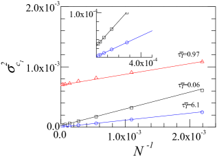
Figure 6: Variance of $c_{I}(t,\tau)$ for a foam, as a function of the inverse number of pixels over which $c_{I}$ is averaged, for three time delays $\tau$. The lines are linear fits to the data for $N^{-1}<5.5\times 10^{-4}$. For $\tau\overline{\gamma}\approx 1$, the intercept of the fit strongly departs from zero, indicating temporarily heterogeneous dynamics as discussed in the text. Note that the fit yields a non-zero intercept also at small delay, as shown in the inset that zooms into the small $\sigma_{c_{I}}^{2}$, large $N$ region. Data were collected in the DWS transmission geometry for a duration $T_{\rm exp}=160$ sec, 242 times longer than the relaxation time of $c_{I}$, $\overline{\gamma}^{-1}=0.33$ sec.

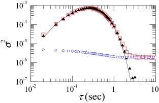
Figure 7: Variance of $c_{I}(t,\tau)$ for a foam, as a function of $\tau$. Open squares: variance of the raw data ($c_{I}$); open circles: noise contribution; solid triangles: $\sigma^{2}_{g_{2}}(\tau)$, the contribution due to the fluctuations of the number of rearrangement events per unit time. The line is a fit to $\sigma^{2}_{g_{2}}(\tau)$ using Eq. (10). Data were collected in the DWS transmission geometry.

IV.2 Correction of the PDF of $c_{I}$

In the absence of intrinsic dynamical fluctuations, knowledge of the average degree of correlation, $\overline{c_{I}}$, and of the noise variance, $\sigma_{n}^{2}$, is sufficient to fully determine the PDF of $c_{I}$ at fixed lag, because $c_{I}$ is a Gaussian variable. Heterogeneous dynamical processes, on the contrary, lead in general to non-Gaussian distributions of $c_{I}(t,\tau)$ Cipelletti et al. (2003); Bissig et al. (2003a); Duri et al. (2005), whose shape depends on both the dynamical process and the time delay $\tau$. Because $c_{I}(t,\tau)$ is the sum of two uncorrelated random variables, $g_{2}(a_{1}(t),...,a_{k}(t);\tau)-1$ and the noise $n(t,\tau)$, the PDF of $c_{I}$ is the convolution of the probability distribution of $g_{2}(a_{1}(t),...,a_{k}(t);\tau)-1$ with that of $n(t,\tau)$ Frieden (2001):

$$P_{c_{I}}(c_{I})=P_{g_{2}-1}(g_{2}-1)\otimes P_{n}(n),$$ (11)

where $P_{x}(x)$ denotes the PDF of $x$ and $(f\otimes g)(x)=\int dx^{\prime}f(x^{\prime})g(x-x^{\prime})$ is the convolution product. In order to recover the physically relevant PDF of $g_{2}-1$ from the measured $P_{c_{I}}(c_{I})$, one may use standard Fourier transform techniques to deconvolute the experimental data, using $P_{n}(n)$ as the response function Press et al. (2002): $P_{g_{2}-1}=\mathcal{F}^{-1}[\mathcal{F}(P_{c_{I}})/\mathcal{F}(P_{n})]$, where $\mathcal{F}$ and $\mathcal{F}^{-1}$ indicate direct and inverse Fourier transform, respectively. Unfortunately, this procedure is very sensitive to noise in the data and leads typically to unstable solutions exhibiting wide oscillations. Instead, we use a technique similar to the indirect Fourier transformation (IFT) method used to process static scattering data. Details on the IFT method can be found in Glatter (1977, 2002), here we simply describe the main steps of our implementation. We first assume that the unknown PDF of $g_{2}-1$ at fixed lag $\tau$ may be written as the linear superposition of a set of suitable functions $\phi_{k}$:

$$P_{g_{2}-1}=\sum_{k=1}^{M}\mu_{k}\phi_{k}(g_{2}-1).$$ (12)

It is convenient to choose $\phi_{k}(x)={\rm rect}(x-x_{k};2\Delta)$, where

$${\rm rect}(x-x_{k};2\Delta)=\left\{\begin{array}[]{r@{\quad: \quad}l}1&|x-x_{k}|\leq\Delta\\ 0&{\rm elsewhere}\end{array}\right.$$ (15)

is a square pulse of width $2\Delta$ centered on $x_{k}$. $2\Delta$ is taken to be the width of the bins used to calculate the PDF of ${c_{I}}$, i.e. the separation between the $c_{I}$ coordinates of the $M$ experimental $P_{c_{I}}$ data. Because the convolution is a linear transformation, Eqs. (11) and (12) yield the following guess for the PDF of $c_{I}$:

$$P_{\rm guess}(c_{I}) = \sum_{k=1}^{M}\mu_{k}{\rm rect}(c_{I}-c_{I,k};\Delta)\otimes P_{n}(c_{I})$$ (16)

$$= \sum_{i=k}^{M}\mu_{k}\sigma^{2}_{n}\sqrt{\frac{\pi}{2}}\left[{\rm erf}(x^{+})-{\rm erf}(x^{-})\right]$$

with

$$x^{\pm}=\frac{1}{\sqrt{2}}\,\sigma^{2}_{n}\left(c_{I}-c_{I,k}\pm\Delta\right).$$ (17)

Here ${\rm erf}(x)=2\pi^{-1/2}\int_{0}^{x}\exp(-u^{2})du$ is the error function Frieden (2001) and $c_{I,k}$ is the center of the $k$-th bin used to calculate the experimental PDF. In writing the last line of Eq. (16) we have used $P_{n}(c_{I})=(2\pi\sigma^{2}_{n})^{-1\!/2}\exp[-c_{I}^{2}/2\sigma^{2}_{n}]$ and calculated explicitly the convolution product. We note that the width of the ${\rm rect}$ functions is typically much smaller than that of the Gaussian noise $P_{n}$, so that the difference of the erf functions in square brackets is very close to a Gaussian. We stress that the only unknowns in Eqs. (16) and (17) are the coefficients $\mu_{k}$, since the variance of the noise $\sigma^{2}_{n}$ can be obtained directly from the experimental $c_{I}$ using the extrapolation scheme described in the preceding subsection.

In principle, the coefficients $\mu_{k}$ can be determined by fitting Eq. (16) to the experimentally measured PDF of $c_{I}$. Once the $\mu_{k}$’s are known, the desired PDF of $g_{2}-1$ can be obtained by using Eq. (12). In practice, two issues must be addressed when determining the set of $\mu_{k}$. Firstly, noise in the experimental $P_{c_{I}}$ can make the fitting procedure unstable. It is therefore convenient to smooth the experimental $P_{c_{I}}$ before fitting it by Eq. (16). To this end, $P_{c_{I}}$ is approximated by a smooth curve, $P_{\rm sm}$, obtained by fitting the data by a suitable function. We find that in most cases

$$P_{\rm sm}(c_{I})=A{\rm e}^{\nu_{1}(c_{I}-c_{0})+\nu_{2}(c_{I}-c_{0})^{2}-\nu_{3}\exp\left[\nu_{4}(c_{I}-c_{0})\right]}$$ (18)

fits well the whole experimental PDF, although fitting $P_{c_{I}}$ piecewise may be sometimes necessary. Note that the Gumbell PDF corresponds to the case $\nu_{1}=\nu_{4}=\alpha>0$, $\nu_{2}=0$, and $\nu_{3}=1$ Chamon et al. (2004). The coefficients $\mu_{k}$ are then found by fitting $P_{\rm guess}(c_{I})$ to $P_{\rm sm}$, rather than directly to $P_{c_{I}}$. Secondly, the PDF of $g_{2}-1$ determined by inserting the $\mu_{k}$’s thus obtained in Eq. (16) often exhibits large oscillations. This is because the erf functions in Eq. (16) do not form an orthogonal basis, as discussed in ref. Glatter (2002). This problem can be solved by adding a stabilization condition when fitting $P_{\rm sm}$ by $P_{\rm guess}$. We follow ref. Glatter (2002) and determine the set of $\mu_{k}$ by minimizing the following expression:

$$\sum_{l=1}^{L}[P_{\rm sm}(c_{I,l})-P_{\rm guess}(c_{I,l})]^{2}+\Lambda\sum_{k=1}^{M-1}(\mu_{k+1}-\mu_{k})^{2}.$$ (19)

The first term in the above expression corresponds to the usual sum of squared deviations between the fitting function ($P_{\rm guess}$) and the data ($P_{\rm sm}$). The second term assigns a cost to any large variation between successive $\mu_{k}$ and thus tends to suppress all fast oscillation of $P_{\rm guess}$. The relative weight of the two terms is controlled by the Lagrange multiplier $\Lambda$, whose optimum value is determined as described in ref. Glatter (2002).

The top panel of fig. 8 shows the PDF of $c_{I}$ measured in the DWS TRC experiment on foam, for $\tau=0.02$ sec (open circles). The solid line is the smoothed PDF, $P_{\rm sm}$, obtained by fitting the data to Eq. (18). The dotted line is the Gaussian PDF of the noise, $P_{n}$, whose width is $\sigma_{n}$ (for display purposes, $P_{n}$ has been centered on $\overline{c_{I}}$, rather than on 0). In the bottom panel, the thick line is the PDF corrected for the noise contribution, $P_{g_{2}-1}$. Note that the right wing of the corrected PDF drops much more abruptly than that of the raw data (for comparison, the uncorrected and the smoothed PDF are also plotted in the bottom panel). The left wing, on the contrary, is almost unaffected by the correction. This is a consequence of the nearly exponential behavior of the left wing: indeed, it can be shown that the convolution of an exponential function with a Gaussian is again exponential, with the same growth rate. We test how close the raw data and the corrected PDF are to a Gumbel distribution by fitting the data to the expression of Eq. (18), with $\nu_{2}=0$ and $\nu_{1}=\nu_{3}\nu_{4}$, corresponding to a generalized Gumbel PDF Chamon et al. (2004). For the raw data, we find $\nu_{3}=1.04$, very close to $\nu_{3}=1$, the value for a Gumbel PDF. By contrast, for the corrected data $\nu_{3}=0.42$, showing that the right wing of the corrected PDF strongly departs from both a Gumbel distribution and the “universal” PDF of ref. Bramwell et al. (2000), for which $\nu_{3}=\pi/2\approx 1.57$. A more detailed investigation of the shape of the PDF of $c_{I}$ for various delays $\tau$ and different systems will be presented elsewhere: here we just stress the importance of the noise correction in view of any quantitative comparison.

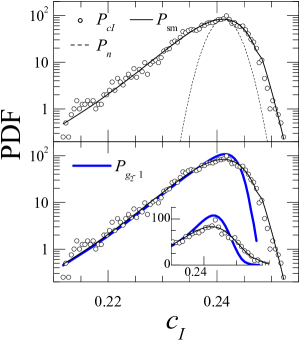
Figure 8: Top panel: PDF of $c_{I}(t,\tau)$ for a foam, for $\tau=0.2$ sec (open circles); data were collected in the DWS transmission geometry. The continuous line is the smoothed distribution, $P_{\rm sm}$, obtained from a fit to Eq. (18). The dotted line is the Gaussian PDF of the noise. Bottom panel: the corrected distribution, $P_{g_{2}-1}$, (thick line), together with the raw data and the smoothed PDF (same symbols as in the top panel). Note the much steeper decay of the right wing of the corrected PDF. The inset shows the data around the peak in a linear axis graph.

IV.3 Direct correction of $c_{I}(t,\tau)$ for $\tau<<\tau_{0}$

The methods developed in subsecs. IV.1 and IV.2 allow one to calculate the variance and the PDF of $g_{2}-1$, but not to correct directly the time-dependent degree of correlation $c_{I}(t,\tau)$. Here we show that such a correction is possible, i.e. that the noise-free $g_{2}(t,\tau)-1$ at fixed $\tau$ may be retrieved as a function of $t$, provided that the following assumptions are fullfilled: $i$) the dynamics is homogeneous on a time scale comparable to the CCD exposure time; $ii$) $\tau<<\tau_{0}$, where $\tau_{0}$ is the average relaxation time of $g_{2}-1$.

We first observe that $c_{I}(t,\tau=0)$ measures the so-called contrast of the speckle pattern, or coherence factor $\beta$. The latter is determined only by the speckle-to-pixel size ratio, which is a time-independent quantity, and by the blurring due to the fluctuations of the speckle during the time the CCD chip is exposed Goodman (1975). If $i$) is fulfilled, the amount of blurring is constant over time and hence $c_{I}(t,0)$ fluctuates only because of the noise . Therefore, $n(t,0)$ can be directly obtained from the experimentally measured $c_{I}(t,0)$:

$$n(t,0)=c_{I}(t,0)-\overline{c_{I}(t,0)}$$ (20)

If in addition also $ii$) is fulfilled, $n(t,\tau)\approx n(t,0)$, because the noise evolves on the same time scale as the speckle pattern, $\tau_{0}$. Indeed, by analyzing TRC data for Brownian particles, we have shown in ref. Duri et al. (2005) that the noise is highly correlated for $\tau<<\tau_{0}$. This suggests that $c_{I}(t,\tau)$ may be directly corrected according to $g_{2}(t,\tau)-1=c_{I}(t,\tau)-n(t,\tau)\approx c_{I}(t,\tau)-n(t,0)$, with $n(t,0)$ obtained via Eq. (20). This approximation may be further refined by taking $n(t,\tau)\approx[n(t,0)+n(t+\tau,0)]/2$ rather than $n(t,\tau)\approx n(t,0)$ and by scaling this estimate of the noise so that its standard deviation matches the actual standard deviation of $n(t,\tau)$:

$$g_{2}(t,\tau)-1 = c_{I}(t,\tau)-[n(t,0)+n(t+\tau,0)]/2$$ (21)

$$\times \sigma_{n}(\tau)/\sigma_{n}(0).$$

Here, the standard deviation of the noise of $c_{I}(t,\tau)$, $\sigma_{n}(\tau)$, is obtained by applying the extrapolation scheme described in subsec. IV.1, while $n(t,0)$ and $n(t+\tau,0)$ are given by Eq. (20) and $\sigma_{n}(0)$ is directly calculated from $n(t,0)$.

We test Eq. (21) on TRC data taken for the dilute suspension of Brownian particles, for which the fluctuations of $c_{I}$ are due only to the measurement noise: $c_{I}(t,\tau)=n(t,\tau)+\overline{c_{I}(t,\tau)}$. The top panel of fig. 9 shows a portion of $c_{I}(t,0)$ and $c_{I}(t,\tau_{1})$, with $\tau_{1}=0.5{\rm~{}sec}<<\tau_{0}=5.8$ sec. Clearly, the two traces are highly correlated, as expected if $n(t,\tau_{1})\approx n(t,0)$. The dotted line is $g_{2}(t,\tau_{1})-1$ calculated according to Eq. (21). Notice that $g_{2}(t,\tau_{1})-1$ is almost constant, as expected for temporally homogeneous dynamics, thus demonstrating the effectiveness of the correction. The bottom panel shows the PDF of $c_{I}(t,\tau_{1})$ and $g_{2}(t,\tau_{1})-1$ calculated over the whole duration of the experiment. By correcting $c_{I}(t,\tau_{1})$ for the noise, its variance is reduced by almost a factor of 100 (from $3.0\times 10^{-5}$ to $3.9\times 10^{-7}$). The residual fluctuations of $g_{2}(t,\tau_{1})$ are most likely due to the noise $\epsilon_{p}(t)$ discussed in reference to Eq. (2), whose variance we estimate to be of the order of $3.9\times 10^{-7}$ .

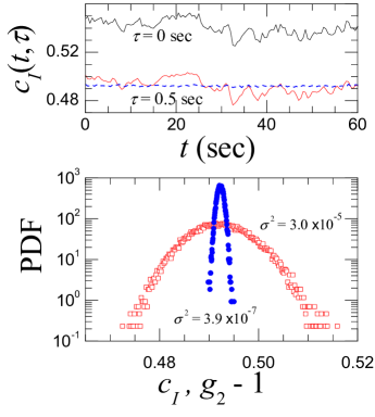
Figure 9: Top panel: $c_{I}(t,0)$ and $c_{I}(t,\tau_{1}=0.5{\rm~{}sec})$ measured for a diluted suspension of Brownian particles, for which the relaxation time of $\overline{g_{2}}-1$ is $\tau_{0}=5.8$. Data are plotted over a short time window to show the strong correlation between the two traces. The dashed blue line is $g_{2}(t,\tau_{1})-1$ obtained by correcting $c_{I}(t,\tau_{1})$ for the noise contribution according to Eq. (21): the fluctuations due to the noise are almost completely removed. Bottom panel: PDF of $c_{I}(t,\tau_{1})$ (open squares) and of $g_{2}(t,\tau_{1})-1$ (solid circles), obtained over the full duration of the experiment ($T_{\rm exp}=10800$ sec). The PDFs are labelled by their variance.

IV.4 Influence of the duration of the experiment

The analysis of the fluctuations of $c_{I}$ presented in subsecs. IV.1 and IV.2 was developed under the assumption that the dynamics be stationary, so that data could be collected over a period, $T_{\rm exp}$, much longer than the average relaxation time of the intensity correlation function, $\tau_{0}$. Dynamical heterogeneity, however, appear to be more prominent for systems close to jamming or quenched in an out-of-equilibrium state. For these systems, meeting the condition $T_{\rm exp}\gg\tau_{0}$ is often impossible, since the sample may be aging, leading to non-stationary dynamics, or because, even if the dynamics is stationary, the relaxation time may be as large as several tens of hours. It is therefore important to address the issue of the influence of the experiment duration on the measured $\sigma_{c_{I}}$.

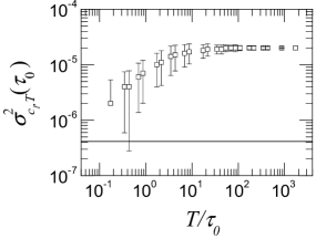
Figure 10: Variance of $c_{I}(t,\tau=\tau_{0})$ calculated over a duration $T$ as a function of $T$ normalized by the mean relaxation time $\tau_{0}$, for a suspension of Brownian particles. A similar behavior is observed for all $\tau$. The line is the contribution to the variance of $c_{I}(t,\tau=\tau_{0})$ of the CCD electronic noise (see the text for more details).

Let us first consider the simpler case of homogeneous dynamics. We divide the time series of $c_{I}(t,\tau)$ obtained for the Brownian particles into non-overlapping segments of duration $T<T_{\rm exp}$. We denote by $\sigma^{2}_{c_{I},T}(\tau)$ the mean value of the variance of $c_{I}(t,\tau)$ calculated for each segment of duration $T$, and plot in fig. 10 $\sigma^{2}_{c_{I},T}$ as a function of $T$ normalized by the relaxation time $\tau_{0}$ (the data refer to $\tau=\tau_{0}$, a similar behavior is observed for all $\tau$). For $T/\tau_{0}>>1$, $\sigma^{2}_{c_{I},T}$ is independent of $T$, because in this regime the experiment duration is long enough for the system (and thus the speckle pattern) to sample a sufficiently large number of different configurations. Consequently, $\sigma^{2}_{c_{I},T}$ saturates to the maximum value given by Eq. (7), which is dictated only by $\tau$ and the number of CCD pixels. Note that for $T/\tau_{0}$ close to one ($T/\tau_{0}=0.87$), $\sigma^{2}_{c_{I},T}$ is still significantly lower than its saturation value (about $35\%$), while it increases to $95\%$ for $T/\tau_{0}>20$ and saturates only for $T/\tau_{0}\geq 50$. As $T/\tau_{0}$ decreases below 1, the amplitude of the fluctuations is significantly reduced when decreasing $T$, since the system is not given enough time to explore significantly different configurations. For $T/\tau_{0}\ll 1$, the speckle pattern is essentially frozen on the time scale of the experiment duration: the fluctuations of $c_{I}$ due to the evolution of the speckle pattern are thus expected to be almost completely suppressed. For the data shown in fig. 10, this regime is not quite reached, since the CCD acquisition rate could not be fast enough to allow for several images to be acquired on a time scale much smaller than $\tau_{0}$ (the smallest lag between images is 0.5 sec = $\tau_{0}/11.6$). In the $T/\tau_{0}\rightarrow 0$ regime, the main contribution to $\sigma^{2}_{c_{I},T}$ should come from the CCD electronic noise $\epsilon_{p}(t)$, whose variance, $\sigma^{2}_{\epsilon}$, is shown as a line in fig. 10. The data shown in this figure clearly demonstrate that care must be taken when comparing the fluctuations measured in experiments whose relative duration $T_{\rm exp}/\tau_{0}$ is different.

For heterogeneous dynamics, we expect the behavior of $\sigma^{2}_{c_{I},T}$ to be qualitatively similar, although the situation will be in general more complicated. In fact, in this case the relevant time scales to which $T_{\rm exp}$ has to be compared are not only the mean relaxation time of $g_{2}-1$, $\tau_{0}$, but also the characteristic time of the “intrinsic” fluctuations of the dynamics, described by the variation of the parameters $a_{1}(t),...a_{k}(t)$ in Eq. (3). As an example, for the foam data shown in figs. 6 and 7 $\tau_{0}=\overline{\gamma(t)}^{~{}-1}=0.32$ sec, while the temporal fluctuations of the decay rate occur on a much longer time scale, $\tau_{\rm fluct}\approx 7$ sec Bissig (2004) (see also fig. 13 below and the associated discussion). Hence, in order to measure precisely the fluctuations the experiment should last more than about $20\tau_{\rm fluct}$, rather than just $20\tau_{0}$. For other jammed materials, on the contrary, the intrinsic fluctuations may be much faster than $\tau_{0}$, as demonstrated by the sudden sharp drops of $c_{I}$ resulting from intermittent rearrangements in a closely packed multilamellar vesicle system Castro-Roman et al. (1999), shown in fig. 11a. In this case, at least for the smallest time lags, the analysis proposed in subsec. IV.3 allows the slow fluctuations due to the measurement noise to be suppressed, while preserving the fast drops of $c_{I}$ that contain the physically relevant information on the dynamical intermittency, as seen in fig. 11b. Note the dramatic change of the shape of the PDF of $c_{I}$ before and after correcting the data, as shown in fig. 11c.

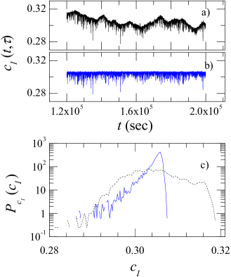
Figure 11: a): time variation of $c_{I}$ for a multilamellar vesicle gel, for $\tau=100$ sec. The mean relaxation time is $\tau_{0}=5050$ sec, the duration of the experiment is $T=80000$ sec = $15.8\times\tau_{0}$. a): raw data; b): the same data after applying the correction Eq. (21); c): PDF of the traces shown in a) (dotted line) and b) (solid line).

V The second correlation

In the previous sections, the fluctuations of $c_{I}$ were analyzed in terms of their variance and PDF. Additional information on the system dynamics can be obtained by studying not only the probability distribution of the fluctuations and its second moment, but also the way these fluctuations occur in time. We characterize the temporal properties of $c_{I}$ at a fixed lag $\tau$ by introducing the time autocorrelation function of $c_{I}(t,\tau)$:

$$C_{c_{I}}(\Delta t,\tau)=\frac{\overline{c_{I}(t,\tau)c_{I}(t+\Delta t,\tau)}-\overline{c_{I}}^{2}}{\overline{c_{I}(t,\tau)^{2}}-\overline{c_{I}}^{2}}.$$ (22)

With this choice of the normalization, $C_{c_{I}}(0,\tau)=1$, and $C_{c_{I}}(\Delta t,\tau)=0$ if $c_{I}(t,\tau)$ and $c_{I}(t+\Delta t,\tau)$ are uncorrelated (e.g. for $\Delta t\rightarrow\infty$). Because $C_{c_{I}}$ is the correlation function of a time-varying quantity –$c_{I}(t,\tau)$– which is obtained itself by correlating the scattered intensity, we shall term it the “second correlation”, in analogy with the “second spectrum” first introduced in the context of spin glasses Weissman (1993). The second spectrum describes in the frequency domain the fluctuations around the mean value of the spectrum of a time-dependent quantity. Similarly, the second correlation describes —in the time domain— the fluctuations of the degree of correlation between the time-dependent system configurations. The second correlation is also similar to the 4-th order intensity correlation function introduced in refs. Lemieux and Durian (1999, 2001), $g^{(4)}_{T}(\tau)=\overline{I(0)I(T)I(\tau)I(\tau+T)}/\overline{I}^{4}$. Note however that $g^{(4)}_{T}(\tau)$ compares the scattered intensity, and thus the sample configuration, at four successive times, while the second correlation compares the $change$ in sample configuration occurring over two time intervals of duration $\tau$ separated by a time $\Delta t$.

As for the case of the PDF discussed in sec. IV, the second correlation contains contributions from both the physically relevant intrinsic fluctuations of $g_{2}(a_{1}(t),...,a_{k}(t);\tau)-1$ and the noise, $n(t,\tau)$. We focus on stationary dynamics measured over a period $T_{\rm exp}\gg\tau_{0}$ and assume that the fluctuations of $g_{2}(a_{1}(t),...,a_{k}(t);\tau)-1$ and $n(t,\tau)$ are uncorrelated: $\overline{g_{2}n}=\overline{g_{2}}\,\overline{n}$ for all $\Delta t$. Under these assumptions and by using Eq. (3), Eq. (22) yields

$$C_{c_{I}}(\Delta t,\tau)=\frac{\sigma^{2}_{g_{2}}(\tau)C_{g_{2}}(\Delta t,\tau)+\sigma^{2}_{n}(\tau)C_{n}(\Delta t,\tau)}{\sigma^{2}_{g_{2}}(\tau)+\sigma^{2}_{n}(\tau)}~{},$$ (23)

where $C_{g_{2}}$ and $C_{n}$ are the correlation functions of the fluctuations of $g_{2}$ and $n$, respectively, defined similarly to Eq. (22). Experiments on Brownian particles (homogeneous dynamics) show that $C_{n}(\Delta t,\tau)\simeq\overline{c_{I}}(\Delta t)/\beta$ for all $\tau$ Duri et al. (2005). Indeed, $C_{n}$ is expected to be proportional to $\overline{c_{I}}$ because the $\tau$ dependence of the noise time autocorrelation stems from the same physical mechanism leading to the decay of the intensity correlation function, i.e. the renewal of the speckle pattern over time discussed in sec. III. In order to extract the desired second correlation of $g_{2}$ from the noise-affected $C_{c_{I}}$, we use a method similar to the extrapolation technique adopted for the calculation of the variance of $g_{2}$. At $\Delta t$ and $\tau$ fixed, $C_{c_{I}}$ depends on the number $N$ of processed pixels through the $\sigma^{2}_{n}$ term in Eq. (23). We omit for simplicity the explicit dependence on $\Delta t$ and $\tau$ and insert Eq. (7) into Eq. (23):

$$C_{c_{I}}(N)=\frac{\sigma^{2}_{g_{2}}C_{g_{2}}+C_{n}N^{-1}\sum_{l=0}^{3}\alpha_{l}\overline{c_{I}}^{l}}{\sigma^{2}_{g_{2}}+N^{-1}\sum_{l=0}^{3}\alpha_{l}\overline{c_{I}}^{l}}$$ (24)

The l.h.s. of this expression can be calculated by processing ROIs of the speckle images of different sizes, as explained in secs. III and IV, and plotted as a function of $N^{-1}$, as shown in fig. 12 for a foam. The r.h.s. of Eq. (24) is then used as a fitting function for $C_{c_{I}}(N)$, where the fitting parameters are the desired $C_{g_{2}}$ and $C_{n}$, while $\sigma^{2}_{g_{2}}$ and $\sum_{l=0}^{3}\alpha_{l}\overline{c_{I}}^{l}$ are obtained independently from the correction of the variance of $c_{I}$, as explained in subsec. IV.1.

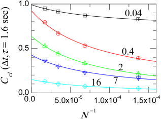
Figure 12: Correction method for $C_{g_{2}}$. Symbols: the second correlation $C_{c_{I}}$ as a function of the inverse number of processed pixels, for various $\Delta t$ (shown by the labels, in sec) and for $\tau=1.6$ sec (only the data for the largest $N$ are shown). The data are obtained from a DWS measurement on a foam. The lines are fits to the data using Eq. (24); the full range of the fit is shown in the figure. The outcome of the fit are the values of $C_{g_{2}}(\Delta t,\tau)$ and $C_{n}(\Delta t,\tau)$ shown with the same symbols in fig. 13.

By repeating this procedure for all $\Delta t$ and $\tau$ of interest, the full second correlation can be corrected for the noise contribution. We show in fig. 13 $C_{g_{2}}(\Delta t,\tau)$ for a foam (open circles), together with the uncorrected data ($C_{c_{I}}$, solid line) and the noise contribution ($C_{n}$, dashed line). Remarkably, a peak is visible in $C_{g_{2}}$, at $\Delta t=\Delta t^{*}\approx 7$ sec. Note that the peak is not present in $C_{n}$, whose only relevant time scale is that of the relaxation of $\overline{c_{I}}$, $\overline{\gamma}^{-1}=0.32$ sec. Therefore, the peak in $C_{g_{2}}$ must be associated with the intrinsic fluctuations of the dynamics due to the intermittent bubble rearrangements. Indeed, the peak indicates that the fluctuations of the instantaneous decay rate $\gamma(t)$ are pseudoperiodic on a time scale of the order of $\Delta t^{*}$. We are currently investigating the origin of this feature.

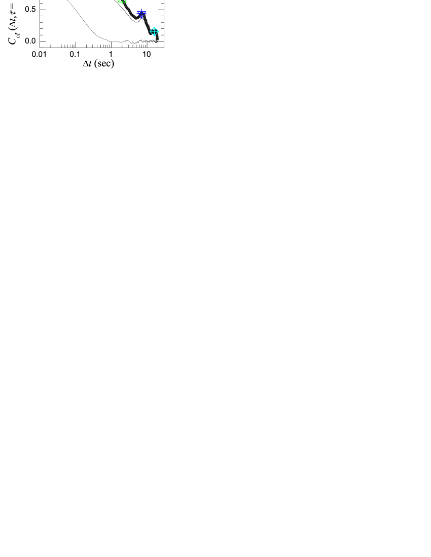
Figure 13: Time autocorrelation function of the fluctuations of $g_{2}$ for a foam, obtained from the second correlation $C_{c_{I}}(\Delta t,\tau)$ by applying the correcting scheme described in the text. Small open circles: the noise-free $C_{g_{2}-1}$; solid line: the experimentally measured $C_{c_{I}}$; dashed line: the noise contribution, $C_{n}$. The large symbols are the values of $C_{g_{2}-1}$ obtained from the fit to the corresponding data shown in fig. 12. Note the peaks of $C_{g_{2}-1}$ at $\Delta t\approx 7$ sec, and $\Delta t\approx 14$ sec, suggesting pseudoperiodic rearrangement events, as discussed in the text.

VI Possible artifacts

In a TRC measurement, the focus is on the fluctuations of the degree of correlation, rather than on its mean value. As a consequence, TRC measurements are very sensitive to various sources of spurious fluctuations, whose effects are usually less prominent or even negligible in traditional dynamic light scattering experiments, since they tend to average out. An example is provided in the top panel of fig. 14, which shows $c_{I}$ measured for the speckle pattern generated in the transmission geometry by a ground glass, a scatterer whose dynamics are completely frozen-in. In this case, we would expect $c_{I}$ to fluctuate slightly only because of the electronic noise $\epsilon_{p}(t)$ discussed in sec. II. Surprisingly, sharp drops of the degree of correlation are clearly visible. Because the drops are rare, they do not affect significantly $\overline{c_{I}}$; however, they do change significantly the PDF of $c_{I}$ and the second correlation. Indeed, one would mistakenly take the dynamics to be intermittent, if the sample was not known. The origin of this artifact is the laser beam pointing instability. Beam pointing instability is the characteristic noise of lasers that results in small fluctuations of the propagation direction of the output beam. Since the speckle pattern is centered around the propagation direction, any change of the incoming beam direction entails a rigid shift of the speckle image with respect to the CCD detector. Thus, the intensity at each pixel slightly changes, leading to a drop of $c_{I}$. To demonstrate that this mechanism is indeed responsible for the sharp drops of $c_{I}$ observed in fig. 14, we show in the bottom panel the corresponding shift, $\Delta r(t,\tau)$, between pairs of images taken at time $t$ and $t+\tau$, measured by Particle Imaging Velocimetry (PIV) Tokumaru and Dimotakis (1995). This method is based on spatial cross-correlation techniques and allows the rigid motion between two images to be quantified with sub-pixel resolution (our adaption of PIV to speckle imaging will be described elsewhere). A comparison between the two panels of fig. 14 clearly shows that the anomalously large drops of $c_{I}$ are due to larger-than-average rigid shifts of the speckle images. Note that shifts as small as a fraction of pixel, corresponding to a few microns, have a measurable impact on $c_{I}$.

Figure 14: Top panel: $c_{I}(t,\tau)$ measured for a static scatterer, a ground glass, for $\tau=5$ sec. Note the sharp drops of the degree of correlation that greatly exceed the noise of the data. Bottom panel: rigid displacement between the pair of speckle images used to calculate $c_{I}(t,\tau)$ above, measured by PIV. The sharp drops of $c_{I}$ are artifacts due to larger-than-average rigid shifts of the speckle images.

This example shows how sensitive to instabilities TRC is. Therefore, care must be taken in order to minimize possible instabilities and to identify any spurious fluctuations of $c_{I}$. Moreover, attempts should be done to correct $c_{I}$ for artifacts. In our experience, the most common artifact encountered in TRC experiments is similar to that exemplified by fig. 14: fluctuations or sharp drops of $c_{I}$ due to a rigid shift of the speckle pattern, rather than to the characteristic “boiling” or flickering of the speckle images associated with the evolution of the sample configuration. In addition to beam pointing instability, temperature variations are often to blame for spurious features in the temporal evolution of $c_{I}$.

Temperature variations may change the direction of propagation of light because of refractive effects, since the refractive index, $n_{\rm D}$, varies with temperature, $T$. As an example, let us consider a typical small-angle single scattering measurement on an aqueous sample contained in a rectangular cell, whose entrance and exit walls are perpendicular to the incoming beam. Light scattered at an angle $\theta_{\rm s}$ equal to, e.g., 15 deg is refracted at the water-to-air interface and exits at an angle given by Snell’s law: $\theta_{\rm air}=\arcsin\left(n_{\rm D}\sin\theta_{\rm s}\right)$ . A temperature fluctuation $\delta T$ induces a variation $\delta\theta_{\rm air}$ given by

$$\delta\theta_{\rm air} = \frac{\partial\theta_{\rm air}}{\partial n_{\rm D}}\frac{\partial n_{\rm D}}{\partial T}\delta T$$ (25)

$$= \frac{\sin\theta_{\rm s}\partial n_{\rm D}/\partial T}{\sqrt{1-\sin^{2}\theta_{\rm s}n_{\rm D}^{2}}}\,\delta T\approx 2.8\times 10^{-5}{\rm~{}rad},$$

where we have used $n_{\rm D}=1.33$, $\frac{\partial n_{\rm D}}{\partial T}\approx 10^{-4}~{}{\rm K}^{-1}$ for water and we have taken $\delta T=1$ K. In a typical small angle setup the sample-to-CCD distance is at least 10 cm and the pixel size is about 10 $\mu$m, resulting in a shift of the speckle associated to the direction $\theta_{\rm s}$ of the order of 0.28 pixels, sufficient to significantly reduce $c_{I}$. Thus temperature fluctuations of the order of 1 K may lead to measurable spurious fluctuations of $c_{I}$ because of refractive effects.

In most single scattering wide-angle apparatuses the sample cell is cylindrical and both the incoming beam and the scattered light cross all optical interfaces at normal incidence, so that refractive effects are avoided. Nevertheless, any change of the refractive index due to temperature variations would still result in a change of the speckle pattern. This is because each speckle is associated to a well defined value of the scattering vector, $\textbf{{q}}_{\rm s}$. If $n_{D}$ changes, the scattering angle $\theta_{\rm s}$ corresponding to $\textbf{{q}}_{\rm s}$ is modified, since $\theta_{\rm s}=2\arcsin\left(\frac{\lambda_{0}q_{\rm s}}{4\pi n_{\rm D}}\right)$, where $\lambda_{0}$ is the laser in-vacuo wavelength. Accordingly, the speckle pattern is contracted or dilated around the $q=0$ direction. This is the same effect as the radial shift of the speckle pattern when changing the wavelength of the incident radiation, which was studied in the Seventies Parry (1974). When only a limited portion of the speckle pattern corresponding to a small solid angle is imaged on the CCD detector (as it is the case, e.g., for the single scattering experiments at $\theta=45$ deg reported in this paper), such a global contraction or dilation results, locally, in a rigid shift of the speckles. The change $\delta\theta_{\rm s}$ of $\theta_{\rm s}$ in response to a temperature fluctuation $\delta T$ is

$$\delta\theta_{\rm s}=\frac{\partial\theta_{\rm s}}{\partial n_{\rm D}}\frac{\partial n_{\rm D}}{\partial T}\delta T$$

$$=\frac{-2\lambda_{0}q_{\rm s}\,\partial n_{\rm D}/\partial T}{n_{\rm D}\sqrt{16\pi^{2}n_{\rm D}^{2}+\lambda_{0}^{2}q_{\rm s}^{2}}}\,\delta T\approx-6.2\times 10^{-5}{\rm~{}rad},$$ (26)

where we have used $n_{\rm D}=1.33$, $\lambda_{0}=0.535$ $\mu{\rm m}$, $q_{\rm s}=12.44$ $\mu{\rm m}^{-1}$ ($\theta_{s}=45$ deg), $\frac{\partial n_{\rm D}}{\partial T}\approx 10^{-4}~{}{\rm K}^{-1}$ and $\delta T=1$ K. Taking the sample-to-CCD distance to be 10 cm, we find that a fluctuation $\delta T=1$ K would result in a shift of the speckle pattern of 6.2 $\mu{\rm m}$, comparable to the pixel size. This would lead to a catastrophic drop of $c_{I}$, since the speckle size is typically of the order of the pixel size. Indeed, even a fluctuation ten time smaller, $\delta T=0.1$ K, would have a measurable impact on $c_{I}$. Similar arguments apply also to multiple scattering experiments. Note that DWS experiments are more sensitive to variations of $n_{D}$ than single scattering measurements are, because minute changes of $q$ at each scattering event add up along the photon path, eventually resulting in a significant change of the phase of scattered photons.

Various strategies are possible to avoid the artifacts discussed above, or at least to mitigate their effects on TRC data. The impact of beam pointing instability can be minimized by reducing as much as possible the light path between the laser and the sample, or by delivering the beam via a fiber optics. In the latter case, beam pointing instability results in fluctuations of the laser-to-fiber coupling efficiency and thus of the incident intensity, $I_{\rm in}$. Because $c_{I}$ is normalized with respect to the instantaneous pixel-averaged intensity (see Eq. 1), fluctuations of $I_{\rm in}$ have little if any effect. Temperature should be controlled at least to within 0.1 K and the sample or sample holder temperature should be monitored, so that any suspect feature in $c_{I}$ could be compared to the temperature record. A PIV analysis similar to that presented in fig. 14 is a useful test to check whether a spurious rigid shift of the speckle pattern is at the origin of large drops of $c_{I}$.

The input from PIV measurements may also be used to correct for the effect of a rigid shift $\Delta\textbf{{r}}$ of the speckle pattern. This could be achieved by constructing a corrected speckle image, shifting back by $-\Delta\textbf{{r}}$ the second image of the pair used to compute $c_{I}$. The corrected image would then be used to calculate $c_{I}$. Standard image-processing techniques Lehmann et al. (1999) can be used to obtain sub-pixel shifts. Alternatively, one may exploit the fact that in the presence of both a rigid shift $\Delta\textbf{{r}}$ and a genuine evolution of the speckle pattern, the measured degree of correlation, $c_{I,{\rm meas}}$, factorizes as $c_{I,{\rm meas}}(t,\tau)=c_{I}(t,\tau)\left[g_{2,{\rm sp}}(\Delta\textbf{{r}})-1\right]$ (a proof is given in the Appendix of ref. Pham et al. (2004)). Here $g_{2,{\rm sp}}(\Delta\textbf{{r}})-1$ is the normalized spatial autocorrelation function of the speckle image and $c_{I}(t,\tau)$ is the degree of correlation that would be measured in the absence of any shift. We are currently exploring both approaches.

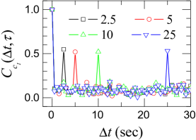
Figure 15: Second correlation measured for a perfectly frozen speckle pattern. The curves are labelled by $\tau$, in sec. Note the spurious peaks at $\Delta t=\tau$, due to the CCD dark noise, as discussed in the text.

We conclude this section by reporting a spurious feature due to the electronic noise $\epsilon_{p}$, which may affect the second correlation $C_{c_{I}}(\Delta t,\tau)$ measured for time lags $\tau$ much smaller than the typical relaxation time. On those short time scales, the speckle pattern is essentially frozen; therefore, we shal use as an example the series of images of a perfectly frozen speckle pattern obtained as described at the end of subsec. IV.3. We process the data as usually and calculate the variance of $c_{I}$. For all lags $\tau>0$ the same value is obtained, which is taken as an estimate of $\sigma^{2}_{\epsilon}$. This has the advantage of excluding other artifacts, such as a possible rigid shift of the speckle pattern. As shown in fig. 15, the second correlation exhibits spikes at $\Delta t=\tau$, emerging form a baseline close to zero. This is a spurious effect due to the fact that the electronic noise $\epsilon_{p}$ is delta-correlated in time. Therefore, $\epsilon_{p}$ contributes an extra term to $\overline{c_{I}(t,\tau)c_{I}(t+\Delta t,\tau)}$ whenever two out of the four intensity terms involved in this expression are measured at the same time, as for $\Delta t=\tau$. A rigorous calculation can be found in ref. Bissig (2004), showing that the height of the spurious peaks is 0.5, in good agreement with fig. 15. The spikes of the second correlation shown in a figure of a (withdrawn) preprint authored by some of us Bissig et al. (2003b) are most likely due to this effect.

VII Conclusions

We have shown that TRC allows heterogeneous dynamics to be unambiguously discriminated from homogeneous dynamics. In order to quantify dynamical heterogeneity, three statistical objects are particularly insightful: the variance of $c_{I}$, which corresponds to the dynamical susceptibility $\chi_{4}$, the PDF of the degree of correlation, and its time autocorrelation function –the second correlation. Statistical noise due to the finite number of pixels over which $c_{I}$ is averaged can contribute significantly to the fluctuations of the degree of correlation. Thanks to the correction scheme described in this paper, the variance, PDF, and time autocorrelation of $c_{I}$ can be corrected for this contribution, thus making quantitative measurements of heterogeneous dynamics accessible to scattering techniques. These corrections are particularly important when the intrinsic fluctuations are comparable to or even smaller than the noise. This may occur because dynamic heterogeneity is mild, e.g. in moderately concentrated suspensions of colloids Ballesta et al. (2005), or because the number of available pixels is reduced, e.g. in a small angle light scattering or XPCS setup, where the lowest accessible $q$ vectors correspond to small rings centered around the transmitted beam and containing a limited number of pixels Cipelletti and Weitz (1999). Corrections are also important when comparing TRC data obtained from different apparatuses, for which both the speckle size and the number of pixels may differ, or when analyzing small angle data, since the number of pixels in the rings associated to different $q$ vectors varies with $q$.

In addition to providing a quantitative description of dynamical fluctuations for systems in a stationary or quasi-stationary state, TRC is a useful tool for studying rapidly evolving dynamics, e.g. during gelation Bissig (2004), as well as the response to an instantaneous perturbation, e.g. an applied shear El Masri et al. (2005). Because in both cases the dynamics may evolve on time scales comparable to or even shorter than the relaxation time of $g_{2}$, a representation of the time evolution of $c_{I}$ is more appropriate and insightful than that of the two-time correlation function. Limitations to the applicability of TRC are mainly due to the CCD acquisition rate, which typically does not exceed a few tens or hundreds of Hz. An additional experimental constraint is the need to store the acquired images on the hard disk of a PC and to process them at the end of the experiment: data sets up to several Gb are not infrequent.

Other techniques have been proposed in the last few years to study dynamical heterogeneity. New light scattering methods include Speckle Visibility Spectroscopy (SVS) Dixon and Durian (2003); Bandyopadhyay et al. (2005) and the measurement of higher order intensity correlation functions Lemieux and Durian (1999, 2001). In a SVS experiment, one measures $c_{I}(t,\tau=0)$, that is the instantaneous contrast —or visibility— of the speckle pattern, $<I_{p}^{2}(t)>_{p}/<I_{p}(t)>_{p}^{2}-1$. The contrast depends on the evolution of the speckle pattern during the exposure (integration) time of the CCD. A significant evolution on this time scale leads to a blurred speckle pattern image, and thus to a reduced contrast. Fluctuations of the contrast can therefore be related to dynamical fluctuations on the time scale of the exposure time. Because the latter is typically much shorter than the time between successive CCD acquisitions, SVS and TRC provide complementary information, on fast and slow dynamics, respectively. Note that SVS data can be obtained on the fly, with no need to store images, since only one image at a time has to be processed. Higher order intensity correlation functions Lemieux and Durian (1999, 2001), calculated by a dedicated hardware, allow one to discriminate between homogeneous and intermittent dynamics. The time scales that are probed and the required measuring time are similar to those in a traditional light scattering experiment: dynamics as fast as a fraction of $\mu$sec can be measured, but the largest available delay is limited to a few tens of seconds and the experiment duration has to be at least 1000 times longer than the largest relaxation time of the system. These constraints limit the applicability to glassy soft matter.

Video and confocal scanning microscopy have been used to study dynamical heterogeneity in concentrated colloidal suspensions Habdas and Weeks (2002). Microscopy and TRC are complementary techniques: while the former provides unsurpassed details on the motion at a single particle level, scattering data typically benefit from better statistics. Additionally, scattering experiments usually require smaller particles than microscopy, a plus when dealing with very slow dynamics and when sedimentation effects should be minimized. Other techniques that can probe heterogeneous behavior in soft glasses are dielectric Buisson et al. (2003) and rheological Bellon et al. (2002) measurements whose sensitivity is pushed to the limits set by thermal fluctuations. The outcome of these experiments shares intriguing similarities with TRC data, such as the non-Gaussian distribution of voltage fluctuations in dielectric measurements on suspensions of Laponite Buisson et al. (2003). Whether these similarities are coincidental or stem from a common physical origin remains an open question.

In the future, a deeper understanding of both spontaneous dynamical fluctuations and the response to external perturbations in soft glassy systems will likely require the combination of different techniques, possibly applied simultaneously on the same sample. We believe that TRC can play an important role in this endeavor, thanks to its ability to detect instantaneous variations in the dynamics.

Appendix A Calculation of the variance and covariance terms in Equation (6)

In this section we provide additional details on the two approaches to the calculation of the variance of the measurement noise mentioned in sec. III. We first show that the variance and covariance terms in Eq. (6) may be expressed in a way that is independent of the homogeneous $vs.$ heterogeneous nature of the dynamics, and then explicitly demonstrate the $N^{-1}$ scaling of $\sigma^{2}_{n}$ that was used in the correction scheme presented in this paper.

The quantities of interest are the variance of the pixel-averaged intensity, $\sigma^{2}_{I}$, the covariance between $I$ and $J$, $\sigma_{I,J}(\tau)$, the variance of the un-normalized intensity correlation function, $\sigma^{2}_{G_{2}}(\tau)$, and the covariance between $G_{2}$ and $I$, $\sigma_{G_{2},I}(\tau)$. We recall that $I(t)=<I_{p}(t)>_{p}$, $J(t)=<I_{p}(t+\tau)>_{p}$ and drop in the following the explicit dependence on $t$ in the notation of all time-varying variables. We assume the dynamics to be stationary and the experiment duration much longer than the average relaxation time of $c_{I}$. We start by noting that $\sigma^{2}_{I}$ quantifies the fluctuations of the $instantaneous$ pixel-averaged intensity. Therefore, $\sigma^{2}_{I}$ is independent of the nature of the dynamics: indeed, any dynamical process that fully renews the speckle pattern will allow all possible values of $I$ to be sampled over time and thus will lead to the same $\sigma^{2}_{I}$. In contrast, $\sigma_{I,J}(\tau)$, $\sigma^{2}_{G_{2}}(\tau)$, and $\sigma_{G_{2},I}(\tau)$ depend on the way the correlation between $distinct$ speckle patterns fluctuates with time and therefore contain contributions due both to the measurement noise and to the intrinsic fluctuations of the dynamics. However, note that the $\tau\rightarrow 0$ and $\tau\rightarrow\infty$ limits of these quantities are insensitive to the dynamics, because they involve either instantaneous properties of the speckle pattern (for $\tau=0$), or quantities related to pairs of speckle images totally uncorrelated (for $\tau\rightarrow\infty$). This observation, together with the linear dependence of $\sigma_{I,J}(\tau)$, $\sigma^{2}_{G_{2}}(\tau)$, and $\sigma_{G_{2},I}(\tau)$ on $\overline{c_{I}}$ in the absence of dynamical heterogeneity shown in fig. 2, suggests the following form for the contribution of the the measurement noise to the covariance and variance terms:

$$\sigma_{I,J}(\tau)=\sigma_{I,J}(\infty)+\frac{\overline{c_{I}(\tau)}}{\beta}\left[\sigma_{I,J}(0)-\sigma_{I,J}(\infty)\right]$$

$$\sigma^{2}_{G_{2}}(\tau)=\sigma^{2}_{G_{2}}(\infty)+\frac{\overline{c_{I}(\tau)}}{\beta}\left[\sigma^{2}_{G_{2}}(0)-\sigma^{2}_{G_{2}}(\infty)\right]$$

$$\sigma_{G_{2},I}(\tau)=\sigma_{G_{2},I}(\infty)$$

$$+\frac{\overline{c_{I}(\tau)}}{\beta}\left[\sigma_{G_{2},I}(0)-\sigma_{G_{2},I}(\infty)\right].$$ (27)

All coefficients in the r.h.s. of the above equations are not affected by dynamical heterogeneity. Table I summarizes their values in terms of quantities that can be directly obtained from the speckle images, regardless of the nature of the dynamics.

Table 1: Coefficients needed to calculate the contribution of the measurement noise to $\sigma_{I,J}(\tau)$, $\sigma^{2}_{G_{2}}(\tau)$, and $\sigma_{G_{2},I}(\tau)$ .

	$\tau=0$	$\tau\rightarrow\infty$
$\sigma_{I,J}(\tau)$	$\sigma^{2}_{I}$	0
$\sigma^{2}_{G_{2}}(\tau)$	$\sigma^{2}_{G_{2}(0)}$	$2\overline{I}^{2}\sigma^{2}_{I}$
$\sigma_{G_{2},I}(\tau)$	$\sigma_{G_{2}(0),I}$	$\overline{I}^{2}\sigma^{2}_{I}$

As mentioned in sec. IV, estimates of $\sigma^{2}_{n}$ obtained by using Eq. (27) and Table I are typically affected by a significant error. In this paper we have proposed a more robust correction method, based on the $N^{-1}$ scaling of the measurement noise variance, which we demonstrate here. For the sake of simplicity, we assume in the following that there is no correlation between the instantaneous value of the intensity at distinct pixels, i.e. $\overline{I_{p}I_{q}}=\overline{I_{p}}~{}\overline{I_{q}}$ for $p\neq q$. Physically, this corresponds to a speckle size much smaller than the pixel size; this requirement considerably simplifies the calculations, but it can be relaxed without changing the $N^{-1}$ scaling, as we shall show at the end of this Appendix.

For experiments whose duration is much longer than the relaxation time of $\overline{c_{I}}$, the intensity at any given pixel fully fluctuates many times and its probability distribution over time is the same as the instantaneous PDF of $I_{p}$ calculated over all $N$ pixels; therefore averages over time and over pixels can be swapped. We take advantage of this property and of the statistical independence between $I_{p}$ and $I_{q}$ to write

$$\sigma^{2}_{I}=\overline{\frac{1}{N^{2}}\sum_{p,q}{I_{p}I_{q}}}-\overline{I}^{2}$$

$$=\frac{1}{N^{2}}\sum_{p=1}^{N}{\overline{I_{p}^{2}}}+\frac{1}{N^{2}}\sum_{p\neq q}{\overline{I_{p}}\,\overline{I_{q}}}-\overline{I}^{2}.$$ (28)

This expression may be further simplified by noting that moments of the intensity at any pixel are equal to those of, let’s say, pixel 1: $\overline{I_{p}^{2}}=\overline{I_{1}^{2}}$ and $\overline{I_{p}}=\overline{I_{1}}=\overline{I}$. Hence

$$\sigma^{2}_{I}=\frac{1}{N}\overline{I_{1}^{2}}+\frac{N(N-1)}{N^{2}}\overline{I}^{2}-\overline{I}^{2}=\frac{1}{N}\overline{I_{1}^{2}}.$$ (29)

Similarly, one obtains

$$\sigma^{2}_{I,J}=\overline{\frac{1}{N^{2}}\sum_{p,q}{I_{p}J_{q}}}-\overline{I}\,\overline{J}$$

$$=\frac{1}{N}\overline{G_{2}}+\frac{N(N-1)}{N^{2}}\overline{I}\,\overline{J}-\overline{I}\,\overline{J}=\frac{1}{N}\overline{c_{I}}\overline{I}^{2},$$ (30)

$$\sigma_{G_{2},I}=\overline{\frac{1}{N^{2}}\sum_{p,q}{I_{p}J_{p}I_{q}}}-\overline{G_{2}}\,\overline{I}$$

$$=\frac{1}{N}\overline{I_{1}^{2}J_{1}}-\frac{1}{N}\overline{G_{2}}\overline{I},$$ (31)

and

$$\sigma^{2}_{G_{2}}=\overline{\frac{1}{N^{2}}\sum_{p,q}{I_{p}J_{p}I_{q}J_{q}}}-\overline{G_{2}}^{2}\,$$

$$=\frac{1}{N}\overline{I_{1}^{2}J_{1}^{2}}-\frac{1}{N}\overline{G_{2}}^{2}.$$ (32)

Equations (29)-(32) show that all the terms in the l.h.s. of the expression of $\sigma_{n}^{2}$, Eq. (6), are indeed proportional to $N^{-1}$.

As a final remark, we show that the form of the equations derived above is not changed by a short-ranged correlation between the intensity of distinct pixels, such as that typically observed in the CCD speckle images. We consider, as an example, the calculation of $\sigma^{2}_{I}$; similar arguments apply also to the other variance and covariance terms. Because the spatial correlation is short-ranged, the intensity of pixel $p$ will be correlated only to that of a small number, $M$, of nearby pixels, whereas for all other pixels $\overline{I_{p}I_{q}}\approx\overline{I_{p}}\,\overline{I_{q}}$. We indicate the set of nearby pixels by $Q_{p}$ and split the double sum over distinct pixels in Eq. (28) as follows:

$$\frac{1}{N^{2}}\sum_{p\neq q}{\overline{I_{p}I_{q}}}=\frac{1}{N^{2}}\sum_{p,q\in Q_{p}}{\overline{I_{p}I_{q}}}+\frac{1}{N^{2}}\sum_{p,q\not\in Q_{p}}{\overline{I_{p}}\,\overline{I_{q}}}$$

$$\approx\frac{1}{N}\sum_{q\in Q_{1}}{\overline{I_{1}I_{q}}}+\frac{N(N-M)}{N^{2}}\overline{I}.$$ (33)

By substituting Eq. (33) in Eq. (28), one finds that $\sigma^{2}_{I}$ still scales as $N^{-1}$, although with a different prefactor:

$$\sigma^{2}_{I}=\frac{1}{N}\overline{I_{1}^{2}}+\frac{1}{N}\sum_{q\in Q_{1}}{\overline{I_{1}I_{q}}}-\frac{M}{N}\overline{I}^{2}.$$ (34)

Appendix B PDF of $c_{I}$

We show here that in the limit of large $N$ and for homogeneous dynamics the PDF of $c_{I}$ is Gaussian, as found experimentally (see fig. 5). Additionally, we will demonstrate the relationship $\overline{G_{2}}=\overline{I}^{2}(\overline{c_{I}}+1)$. Note that this relationship is not trivial, since in general $(\overline{c_{I}}+1)=\overline{\left[\frac{<I_{p}J_{p}>_{p}}{IJ}\right]}$ differs from $\frac{\overline{<I_{p}J_{p}>_{p}}}{\overline{I}\,\overline{J}}=\frac{\overline{G_{2}}}{\overline{I}^{2}}$.

We start by noting that $G_{2}$, $I$, and $J$ are obtained from an average over a large number $N$ of pixels. Because of the central limit theorem, their PDF is Gaussian, with a standard deviation much smaller than the mean. Accordingly, at any time $G_{2}(t)=\overline{G_{2}}\left[1+\epsilon_{G_{2}}(t)\right]$, with $\epsilon_{G_{2}}$ a Gaussian distributed random variable with mean $\overline{\epsilon_{G_{2}}}=0$ and variance $\sim N^{-1}$. One can write similar expressions for $I(t)$ and $J(t)$, so that to leading order

$$\frac{G_{2}}{IJ}=\frac{\overline{G_{2}}(1+\epsilon_{G_{2}})}{\overline{I}(1+\epsilon_{I})\overline{J}(1+\epsilon_{J})}\approx\frac{\overline{G_{2}}}{\overline{I}^{2}}(1+\xi),$$ (35)

where we have used $\overline{J}=\overline{I}$ and have introduced $\xi=\epsilon_{G_{2}}-\epsilon_{I}-\epsilon_{J}$. $\xi$ is the sum of three (partially correlated) Gaussian random variables and therefore is itself Gaussian distributed Frieden (2001), with mean $\overline{\epsilon_{G_{2}}}-\overline{\epsilon_{I}}-\overline{\epsilon_{J}}=0$. It follows that the PDF of

$$c_{I}=\frac{G_{2}}{IJ}-1\approx\frac{\overline{G_{2}}}{\overline{I}^{2}}(1+\xi)-1$$ (36)

is Gaussian, with mean $\overline{c_{I}}=\frac{\overline{G_{2}}}{\overline{I}^{2}}-1$. Thus, $\overline{G_{2}}=\overline{I}^{2}(\overline{c_{I}}+1)$.

References

- Cipelletti and Ramos (2005) L. Cipelletti and L. Ramos, J. Phys.: Condens. Matter 17, R253 (2005).
- Dawson et al. (2001) K. Dawson, G. Foffi, M. Fuchs, W. Gotze, F. Sciortino, M. Sperl, P. Tartaglia, T. Voigtmann, and E. Zaccarelli, Phys. Rev. E 63, 011401 (2001).
- Eckert and Bartsch (2002) T. Eckert and E. Bartsch, Phys. Rev. Lett. 89, 125701 (2002).
- Pham et al. (2002) K. N. Pham, A. M. Puertas, J. Bergenholtz, S. U. Egelhaaf, A. Moussaid, P. N. Pusey, A. B. Schofield, M. E. Cates, M. Fuchs, and W. C. K. Poon, Science 296, 104 (2002).
- Liu and Nagel (1998) A. Liu and S. Nagel, Nature 396, 21 (1998).
- Cipelletti et al. (2000) L. Cipelletti, S. Manley, R. C. Ball, and D. A. Weitz, Phys. Rev. Lett. 84, 2275 (2000).
- Knaebel et al. (2000) A. Knaebel, M. Bellor, J. P. Munch, V. Viasnoff, F. Lequeux, and J. L. Harden, Europhys. Lett. 52, 73 (2000).
- Viasnoff and Lequeux (2002) V. Viasnoff and F. Lequeux, Phys. Rev. Lett. 89, 065701 (2002).
- Bonn et al. (2002) D. Bonn, S. Tanase, B. Abou, H. Tanaka, and J. Meunier, Phys. Rev. Lett. 89, 015701 (2002).
- Weeks et al. (2000) E. Weeks, J. Crocker, A. Levitt, A. Schofield, and D. Weitz, Science 287, 627 (2000).
- Kegel and van Blaaderen (2000) W. K. Kegel and A. van Blaaderen, Science 287, 290 (2000).
- Mayer et al. (2004) P. Mayer, H. Bissig, L. Berthier, L. Cipelletti, J. P. Garrahan, P. Sollich, and V. Trappe, Phys. Rev. Lett. 93, 115701 (2004).
- Berne and Pecora (1976) B. J. Berne and R. Pecora, Dynamic Light Scattering (Wiley, New York, 1976).
- Goodman (1975) J. W. Goodman, in Laser speckles and related phenomena, edited by J. C. Dainty (Springer-Verlag, Berlin, 1975), vol. 9 of Topics in Applied Physics, p. 9.
- Weitz and Pine (1993) D. A. Weitz and D. J. Pine, in Dynamic Light scattering, edited by W. Brown (Clarendon Press, Oxford, 1993), p. 652.
- Muller and Palberg (1996) J. Muller and T. Palberg, Prog. Colloid Polym. Sci. 100, 121 (1996).
- Pham et al. (2004) K. N. Pham, S. U. Egelhaaf, A. Moussaid, and P. N. Pusey, Rev. Sci. Instrum. 75, 2419 (2004).
- Wong and Wiltzius (1993) A. P. Y. Wong and P. Wiltzius, Rev. Sci. Instrum. 64, 2547 (1993).
- Kirsch et al. (1996) S. Kirsch, V. Frenz, W. Schartl, E. Bartsch, and H. Sillescu, J. Chem. Phys. 104, 1758 (1996).
- Cipelletti and Weitz (1999) L. Cipelletti and D. A. Weitz, Rev. Sci. Instrum. 70, 3214 (1999).
- Cipelletti et al. (2003) L. Cipelletti, H. Bissig, V. Trappe, P. Ballesta, and S. Mazoyer, J. Phys.: Condens. Matter 15, S257 (2003).
- Viasnoff et al. (2002) V. Viasnoff, F. Lequeux, and D. J. Pine, Rev. Sci. Instrum. 73, 2336 (2002).
- Cardinaux et al. (2002) F. Cardinaux, L. Cipelletti, F. Scheffold, and P. Schurtenberger, Europhys. Lett. 57, 738 (2002).
- Diat et al. (1998) O. Diat, T. Narayanan, D. L. Abernathy, and G. Grubel, Curr. Opin. Colloid Interface Sci. 3, 305 (1998).
- Cowan et al. (2002) M. L. Cowan, I. P. Jones, J. H. Page, and D. A. Weitz, Phys. Rev. E 65, 066605 (2002).
- Lacevic et al. (2003) N. Lačević, F. W. Starr, T. B. Schroder, and S. C. Glotzer, J. Chem. Phys. 119, 7372 (2003).
- Whitelam et al. (2005) S. Whitelam, L. Berthier, and J. P. Garrahan, Phys. Rev. E 71, 026128 (2005).
- Pitard (2005) E. Pitard, Phys. Rev. E 71, 041504 (2005).
- de Candia et al. (2005) A. de Candia, E. Del Gado, A. Fierro, N. Sator, and A. Coniglio, preprint cond-mat/0312591 (2005).
- Lacevic et al. (2002) N. Lacevic, F. W. Starr, T. B. Schroder, V. N. Novikov, and S. C. Glotzer, Phys. Rev. E 66 (2002).
- Bissig et al. (2003a) H. Bissig, S. Romer, L. Cipelletti, V. Trappe, and P. Schurtenberger, Phys. Chem. Comm. 6, 21 (2003a).
- Sarcia and Hebraud (2005) R. Sarcia and P. Hebraud, Phys. Rev. E 72, 011402 (2005).
- Ballesta et al. (2004) P. Ballesta, C. Ligoure, and L. Cipelletti, AIP Conf. Proc. 708, 68 (2004).
- Duri et al. (2005) A. Duri, P. Ballesta, L. Cipelletti, H. Bissig, and V. Trappe, Fluctuation and Noise Letters 5, L1 (2005).
- Bissig (2004) H. Bissig, Phd thesis, University of Fribourg (2004), also available at http://www.unifr.ch/physics/mm/index.php.
- Caballero et al. (2004) G. Caballero, A. A. Lindner, G. Ovarlez, G. Reydellet, J. Lanuza, and E. Clement, preprint cond-mat/0403604 (2004).
- Chamon et al. (2004) C. Chamon, P. Charbonneau, L. F. Cugliandolo, D. R. Reichman, and M. Sellitto, J. Chem. Phys. 121, 10120 (2004).
- Clusel et al. (2004) M. Clusel, J.-Y. Fortin, and P. C. W. Holdsworth, Phys. Rev. E 70, 046112 (2004).
- Merolle et al. (2005) M. Merolle, J. P. Garrahan, and D. Chandler, Proc. Natl. Acad. Sci. U. S. A. 102, 10837 10840 (2005).
- Crisanti and Ritort (2004) A. Crisanti and F. Ritort, Europhys. Lett. 66, 253 (2004).
- Bramwell et al. (2000) S. T. Bramwell, K. Christensen, J.-Y. Fortin, P. C. W. Holdsworth, H. J. Jensen, S. Lise, J. M. Lopez, M. Nicodemi, J.-F. Pinton, and M. Sellitto, Phys. Rev. Lett. 84, 3744 (2000).
- Lemieux and Durian (1999) P. A. Lemieux and D. J. Durian, J. Opt. Soc. Am. A 16, 1651 (1999).
- Lemieux and Durian (2001) P. A. Lemieux and D. J. Durian, Appl. Opt. 40, 3984 (2001).
- Schmidtrohr and Spiess (1991) K. Schmidt-Rohr and H. W. Spiess, Phys. Rev. Lett. 66, 3020 (1991).
- Weissman (1993) M. B. Weissman, Reviews of Modern Physics 65, 829 (1993).
- Durian et al. (1991) D. J. Durian, D. J. Pine, and D. A. Weitz, Science 252, 686 (1991).
- Frieden (2001) B. R. Frieden, Probability, statistical optics, and data testing (Springer, Berlin, 2001), 3rd ed.
- Press et al. (2002) W. H. Press, B. P. Flannery, S. A. Teukolsky, and W. T. Vetterling, Numerical Recipes in C++ : The Art of Scientific Computing (Cambridge University Press, Cambridge, 2002), 2nd ed.
- Glatter (1977) O. Glatter, J. Appl. Crystallogr. 10, 415 (1977).
- Glatter (2002) O. Glatter, in Neutrons, X-rays and light: scattering methods applied to soft condensed matter, edited by P. Lindner and T. Zemb (North-Holland, Amsterdam, 2002), Delta.
- Castro-Roman et al. (1999) F. Castro-Roman, G. Porte, and C. Ligoure, Phys. Rev. Lett. 82, 109 (1999).
- Tokumaru and Dimotakis (1995) P. T. Tokumaru and P. E. Dimotakis, Experiments in Fluids 19, 1 (1995).
- Parry (1974) G. Parry, Opt. Commun. 12, 75 (1974).
- Lehmann et al. (1999) T. M. Lehmann, C. Gonner, and K. Spitzer, Ieee Transactions on Medical Imaging 18, 1049 (1999).
- Bissig et al. (2003b) H. Bissig, V. Trappe, S. Romer, and L. Cipelletti, preprint cond-mat/0301265 (2003b).
- Ballesta et al. (2005) P. Ballesta, A. Duri, and L. Cipelletti, in preparation (2005).
- El Masri et al. (2005) D. El Masri, M. Pierno, L. Berthier, and L. Cipelletti, e-print cond-mat/0506527 (2005).
- Dixon and Durian (2003) P. K. Dixon and D. J. Durian, Phys. Rev. Lett. 90 , 184302 (2003).
- Bandyopadhyay et al. (2005) R. Bandyopadhyay, A. Gittings, S. Suh, P. Dixon, and D. J. Durian, preprint cond-mat/0506081 (2005).
- Habdas and Weeks (2002) P. Habdas and E. R. Weeks, Curr. Opin. Colloid Interface Sci. 7, 196 (2002).
- Buisson et al. (2003) L. Buisson, L. Bellon, and S. Ciliberto, J. Phys.: Condens. Matter 15, S1163 (2003).
- Bellon et al. (2002) L. Bellon, L. Buisson, S. Ciliberto, and F. Vittoz, Rev. Sci. Instrum. 73, 3286 (2002).