Charge carrier correlation in the electron-doped $t$-$J$ model

Abstract

We study the $t$-$t^{\prime}$-$t^{\prime\prime}$-$J$ model with parameters chosen to model an electron-doped high temperature superconductor. The model with one, two and four charge carriers is solved on a 32-site lattice using exact diagonalization. Our results demonstrate that at doping levels up to $x=0.125$ the model possesses robust antiferromagnetic correlation. When doped with one charge carrier, the ground state has momenta $(\pm\pi,0)$ and $(0,\pm\pi)$. On further doping, charge carriers are unbound and the momentum distribution function can be constructed from that of the single-carrier ground state. The Fermi surface resembles that of small pockets at single charge carrier ground state momenta, which is the expected result in a lightly doped antiferromagnet. This feature persists upon doping up to the largest doping level we achieved. We therefore do not observe the Fermi surface changing shape at doping levels up to 0.125.

I Introduction

It is well known that electron-doped high $T_{c}$ materials have very different properties compared to hole-doped ones. Like hole-doped materials, their undoped parent compounds are insulators with antiferromagnetic spin order. But the electron-doped cuprate $\text{Nd}_{2-x}\text{Ce}_{x}\text{CuO}_{4}$ remains an antiferromagnetic insulator up to doping level $x=0.13$ whereas in the hole-doped cuprate $\text{La}_{2-x}\text{Sr}_{x}\text{CuO}_{4}$ a relative small doping level of $x\sim 0.02$ is enough to destroy its antiferromagnetic correlation.d94 Theoretically it has been postulated that this asymmetry in properties of electron- and hole-doped materials can be modeled by adding intra-sublattice hopping terms to the $t$-$J$ model.tm94 ; gvl94 Compared to the nearest neighbor hopping motion in the $t$-$J$ model, intra-sublattice hoppings do not frustrate the spin background. Consequently the antiferromagnetic order of the undoped system is better preserved upon doping. Within this context, various theoretical and numerical studies have confirmed that the electron-doped model has robust antiferromagnetic order. In addition, appropriate intra-sublattice hopping terms shift single-carrier ground state momenta from $(\pm\pi/2,\pm\pi/2)$ in the $t$-$J$ model to $(\pi,0)$ and its equivalent points. This means that in a lightly doped system small charge carrier pockets will form at $(\pi,0)$ and its equivalent points in the first Brillouin zone. This agrees with angle-resolved photoemission (ARPES) experimenta02 ; dhs03 on $\text{Nd}_{2-x}\text{Ce}_{x}\text{CuO}_{4}$. Various properties of the electron-doped modeltm01 ; tm03 ; t04 ; yclt04 ; ylt05 including its electronic states, spin dynamics, and Fermi surface evolution have been worked out with emphasis on comparison with experimental results.hubbard

In this paper we are interested in the interaction among charge carriers doped into the parent compound. For this reason we conduct a systematic study on the electron-doped model with a few charge carriers using exact diagonalization. In this approach, larger lattices are always preferred in order to minimize finite-size effects. Furthermore, in order to study Fermi surface evolution the lattice must have allowed k points along the antiferromagnetic Brillouin zone (AFBZ) boundary, i.e., from $(\pi,0)$ to $(0,\pi)$. Square lattices having only 20 or 26 sites with periodic boundary conditions do not have this property. The 32-site lattice is the next available square lattice that has this property and on which calculations are still manageable. The $t$-$J$ model with up to four charge carriers on this lattice has been studied in detail using exact diagonalization.lg95 ; clg98 ; l02 ; l05 But previous calculations on the electron-doped model on this lattice have been limited to two charge carriers only.ln23 Since antiferromagnetic order in electron-doped cuprates is robust, we need more charge carriers to make the antiferromagnetic phase unstable. In this paper we report results for the electron-doped model with one, two, and four charge carriers on a 32-site lattice, covering doping levels up to $x=0.125$.

Our paper is organized as follows. We first define the model in section II. In section III we look at quasiparticle properties of a single charge carrier doped into the system. Next we consider systems with multiple charge carriers and study the binding energies in section IV and the real space charge carrier correlation in section V. They provide the first evidence that charge carriers are unbound at these doping levels. Section VI deals with the momentum distributions of spin objects which indicates the Fermi surface at different doping levels. In section VII we calculate the spin correlations which clearly demonstrate that antiferromagnetic order persists upon doping, and in section VIII we attempt to search for other exotic order when the antiferromagnetic correlation is weakened. Finally we give our conclusion in section IX.

II Hole- and electron-doped models

We start from the extended $t$-$J$ model which was originally proposed to describe hole-doped materials,

$${\cal H}=-\sum_{\langle ij\rangle\sigma}t_{ij}(\tilde{c}^{\dagger}_{i\sigma}\tilde{c}_{j\sigma}+\tilde{c}^{\dagger}_{j\sigma}\tilde{c}_{i\sigma})+J\sum_{nn}\left({\bf S}_{i}\cdot{\bf S}_{j}-\frac{1}{4}n_{i}n_{j}\right).$$ (1)

The nearest neighbor (nn) spin exchange constant $J$ is fixed at $0.3$. Farther than nearest neighbor hopping terms are necessary in order to distinguish between hole and electron doping. $t_{ij}=t,t^{\prime},$ and $t^{\prime\prime}$ when $\langle ij\rangle$ is a pair of sites at distances 1, $\sqrt{2}$, and 2 apart respectively, and is zero otherwise. The best fitting to ARPES results on $\text{Sr}_{2}\text{CuO}_{2}\text{Cl}_{2}$ yields $t=1$, $t^{\prime}=-0.3$, and $t^{\prime\prime}=0.2$.lwg97 In the case of hole doping, $\tilde{c}^{\dagger}_{i\sigma}$ is a spin (or electron) creation operator . To describe electron-doped materials it is usual to apply the electron-hole transformation,gvl94 $\tilde{c}_{i\sigma}\rightarrow\tilde{a}^{\dagger}_{i\sigma}$, where $\tilde{a}^{\dagger}_{i\sigma}$ is a hole creation operator. The resulting Hamiltonian for electron-doped materials is identical to (1) but with $\tilde{c}_{i\sigma}$ replaced by $\tilde{a}_{i\sigma}$, etc, and $t_{ij}$ replaced by $-t_{ij}$. As a result we can turn the Hamiltonian (1) into an electron-doped model by flipping the signs of the hopping terms $t_{ij}$.tm94 Despite this similarity, one should be reminded that in the case of hole doping the operators $\tilde{c}_{i\sigma}$ in the Hamiltonian are electron operators and the vacuum state is a state with no electron. The condition of no double occupancy means that no more than one electron can occupy the same site. At half-filling, each site has exactly one electron and doping with holes means creating vacancies by removing electrons. Translating into the language of the electron-doped model, the operators $\tilde{c}_{i\sigma}$ are hole operators and the vacuum state is a state with no hole, i.e., it cannot accommodate any more electron. The condition of no double occupancy means that each site can have no more than one hole. At half-filling, each site has exactly one hole and doping means filling up holes with electrons. To avoid confusion, we use the terms “spin objects” and “charge carriers” to describe objects in the Hamiltonian (1). In the case of hole doping, spin objects refer to electrons and charge carriers refer to holes. In the case of electron doping their meanings are reversed — spin objects refer to holes and charge carriers refer to electrons. In this paper, by “electron-doped model” we mean (1) with hopping parameters $t=-1$, $t^{\prime}=0.3$, and $t^{\prime\prime}=-0.2$. [edope_number, ] In principle hole-doped model should refer to the same extended $t$-$J$ model with $t=1$, $t^{\prime}=-0.3$, and $t^{\prime\prime}=0.2$. But due to complications caused by excited states of that model,l02 we choose to compare the electron-doped model with the simple $t$-$J$ model, i.e., with $t=1$ and $t^{\prime}=t^{\prime\prime}=0$. We remark that the $t$-$J$ model was originally proposed to describe hole-doped materials. But since they have different hopping terms, it will be unfair to conduct a quantitative comparison between the $t$-$J$ and electron-doped models. Instead we will mostly concentrate on their qualitative differences.

The electron-doped model with Hamiltonian (1) and parameters $J=0.3$, $t=-1$, $t^{\prime}=0.3$, and $t^{\prime\prime}=-0.2$ is solved by exact diagonalization on a square lattice with 32 sites and periodic boundary conditions. Table 1 shows the ground state energies and symmetries of the electron-doped model with one, two, and four electrons. Calculations on the model with four electrons were performed on a cluster of AMD Opteron servers with 64 CPUs.

Table 1: Ground state energies, momenta and point group symmetries of the electron-doped model with $N_{c}$ charge carriers. $N_{B}$ is the number of basis in that particular subspace. The ground state energy at half-filling $E^{0}_{0}$ is $-11.329720$.

$N_{c}$	$N_{B}$	$E^{N_{c}}_{0}$	k	symmetry
1	150,297,603	$-13.913616$	$(\pi,0)$,$(0,\pi)$
2	150,295,402	$-16.601689$	$(0,0)$	$d_{x^{2}-y^{2}}$
4	2,817,694,064	$-20.461647$	$(0,0)$	$s$

III Quasi-particle dispersion in the one-electron system

In the electron-doped model the spectral function of spin objects at half-filling is defined asaq

$$A({\bf k},\omega)=\sum_{n}|\langle\psi^{1}_{n}|\tilde{c}_{{\bf k}\sigma}|\psi^{0}_{0}\rangle|^{2}\delta(\omega-E^{1}_{n}+E^{0}_{0}),$$ (2)

where $E^{0}_{0}$ and $\psi^{0}_{0}$ are the ground state energy and wave function of the model at half-filling, and $E^{1}_{n}$ and $\psi^{1}_{n}$ are energy and wave function of the $n$th excited state of the model with one charge carrier. $A({\bf k},\omega)$ can be evaluated easily using the continued fraction expansion. At each k point we use 300 iterations and add an artificial broadening factor $\epsilon=0.05$ to the delta function. Fig. 1 shows $A({\bf k},\omega)$ along three branches in the first Brillouin zone. At the Brillouin zone center $(0,0)$, the spectral function has a broad structure. It does not have any noticeable low energy peaks. As we move along the $(1,1)$ direction towards $(\pi,\pi)$ [Fig. 1(a)] the spectral weight spreads to lower and higher energies, forming well-defined peaks at low energies. When we go pass $(\pi/2,\pi/2)$, the reverse occurs and at $(\pi,\pi)$, the spectral function has a broad structure again. A similar trend is observed in the branch from $(0,0)$ to $(\pi,\pi)$ through $(\pi,0)$ [Fig. 1(b)]. This branch has the largest dispersion. A different trend is observed along the AFBZ boundary, $(\pi,0)$ to $(0,\pi)$ [Fig. 1(c)]. There the spectral weight mostly concentrates in low energy states. As usual we define the quasiparticle weight $Z_{\bf k}$ as

$$Z_{\bf k}=\frac{|\langle\psi^{1}_{n}|\tilde{c}_{{\bf k}\sigma}|\psi^{0}_{0}\rangle|^{2}}{\langle\psi^{0}_{0}|\tilde{c}^{\dagger}_{{\bf k}\sigma}\tilde{c}_{{\bf k}\sigma}|\psi^{0}_{0}\rangle},$$ (3)

where $\psi^{1}_{n}$ is the lowest energy one-electron state which has non-zero overlap with $\tilde{c}_{{\bf k}\sigma}|\psi^{0}_{0}\rangle$. These values are tabulated in Table 2 together with the quasiparticle energy,

$$E({\bf k})=E^{1}_{n}-E^{0}_{0},$$ (4)

which is the energy of the state $\psi^{1}_{n}$ in Eq.(3) relative to the ground state energy at half-filling. Most $Z_{\bf k}$ are too small to make their corresponding peaks visible in Fig. 1. Their positions are indicated by shaded arrows. An obvious exception is ${\bf k}=(\pi,0)$ which is the ground state momentum of the one-electron system. There the lowest energy peak has more than 60% of the total spectral weight. The quasiparticle energy is plotted in Fig. 2. The bandwidth is $3.777J$, which is in qualitative agreement with the prediction of spin-polaron calculation.bcs96

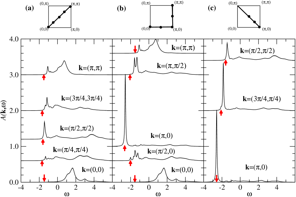
Figure 1: (Color online) Spectral function at half-filling $A({\bf k},\omega)$ along three branches: a) $(0,0)$ to $(\pi,\pi)$, b) $(0,0)$ to $(\pi,0)$ to $(\pi,\pi)$, and c) $(\pi,0)$ to $(0,\pi)$. Shaded arrows indicate the quasiparticle energy $E({\bf k})$.

Table 2: Quasiparticle energy and weight in the electron-doped model.

k	$E({\bf k})$	$Z_{\bf k}$
(0,0)	$-1.452767$	$0.00008$
($\frac{\pi}{4}$,$\frac{\pi}{4}$)	$-1.689698$	$0.00354$
($\frac{\pi}{2}$,$\frac{\pi}{2}$)	$-1.596649$	$0.00465$
($\frac{3\pi}{4}$,$\frac{3\pi}{4}$)	$-1.669586$	$0.00045$
($\pi$,$\pi$)	$-1.450790$	$0.00005$
($\pi$,$\frac{\pi}{2}$)	$-1.986268$	$0.00237$
($\pi$,0)	$-2.583895$	$0.63608$
($\frac{\pi}{2}$,0)	$-2.007321$	$0.02755$
($\frac{3\pi}{4}$,$\frac{\pi}{4}$)	$-2.092922$	$0.01890$

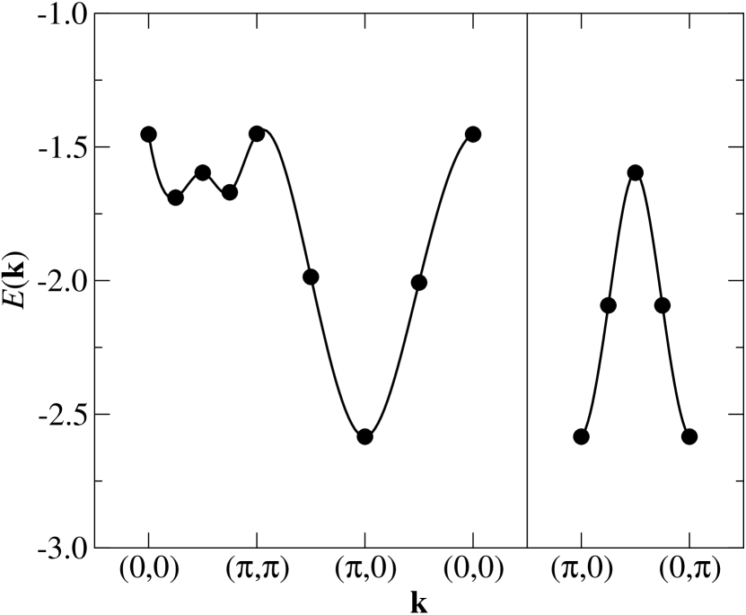
Figure 2: Quasiparticle dispersion relation obtained from the spectral function at half-filling in Fig. 1. The line is a guide to the eyes only.

IV Binding energy

The $N_{c}$-charge carrier binding energy is defined as the excess energy of a system with $N_{c}$ charge carriers over $N_{c}$ single-carrier systems,ry89

$$E_{N_{c}I}\equiv(E^{N_{c}}_{0}-E^{0}_{0})-N_{c}(E^{1}_{0}-E^{0}_{0}).$$ (5)

It indicates the tendency of the $N_{c}$ charge carriers to form a bound state. From values in Table 1 we find that $E_{2I}=-0.1042$ and $E_{4I}=1.2037$. Compared to the $t$-$J$ model where $E_{2I}=-0.0515$,clg98 it is tempting to interpret these numbers as evidence showing that two charge carriers in the electron-doped model have larger tendency to form a bound pair than in the $t$-$J$ model. However, we have two reasons to believe that this is not a fair conclusion. First of all we should not compare the tendency to form bound pairs in the two models based on the magnitudes of their binding energies because they have different hopping terms. As we shall see in the next section, two charge carriers in the electron-doped model in fact have a smaller tendency to form a bound state than in the $t$-$J$ model. Second, one must be careful in interpreting binding energies defined in Eq. (5) because they are very susceptible to finite-size effects. Binding energies found in a finite system tend to be lower than their true values in the thermodynamic limit. As already pointed out in Ref. clg98, , we have no a priori reason to believe that $E_{2I}$ can be extrapolated linearly in $1/N$, where $N$ is the lattice size. Nevertheless, doing so with results at $N=16$ and 32 we obtain $E_{2I}\sim-0.01$. This small value already hinted that the charge carriers may not form a bound state. When there are four charge carriers in the system, the large and positive $E_{4I}$ clearly shows that they have no tendency to form a bound state.

V charge carrier correlation in Real space

The real space correlation among charge carriers can be clearly displayed in the charge carrier correlation function

$$C(r)=\langle(1-n_{r})(1-n_{0})\rangle,$$ (6)

where $n_{r}\equiv\tilde{c}^{\dagger}_{r}\tilde{c}_{r}$ is the number operator of spin objects as in Eq. (1). Note that we use the conventionclg98

$$C(r)=\frac{1}{N_{c}N_{E}(r)}\sum_{ij}\bigl{\langle}(1-n_{i})(1-n_{j})\delta_{|i-j|,r}\bigr{\rangle},$$ (7)

where $N_{E}(r)$ is the number of equivalent pairs with separation $r$. In this convention the correlation function satisfies the sum rule

$$\sum_{r>0}N_{E}(r)C(r)=N_{c}-1,$$ (8)

and the probability for finding a pair of charge carriers at distance $r$ apart is

$$P(r)=N_{E}(r)C(r)/(N_{c}-1).$$ (9)

Results in the two- and four-electron systems are shown in Fig. 3. Note that we use different symbols to distinguish between two groups of correlations – those between pairs of electrons in the same and opposite sublattices. A striking feature in the two-electron system is that the correlation between two electrons in opposite sublattices does not decay significantly with $r$. It is almost constant, implying that electrons in opposite sublattices are mostly uncorrelated. The correlation between two electrons in the same sublattice shows a very different trend. It is comparatively smaller than that in the other group and decays more significantly with distance $r$. The overall probability of finding a pair of electrons in the same and opposite sublattices are $0.3935$ and $0.6065$ respectively. From these results we conclude that in the two-electron system, electrons prefer to stay in opposite sublattices where they can move almost independently of each other. Obviously this results from the fact that intra-sublattice hopping terms $t^{\prime}$ and $t^{\prime\prime}$ in ${\cal H}$ do not frustrate the spin background and therefore allow electrons to move more freely. When we increase the number of electrons to four, the behaviors of the two groups of correlation become very similar. They show small fluctuations about the uncorrelated value $(N_{c}-1)/(N-1)$, which is indicated by a dotted line in Fig. 3. This shows that even in the four-electron system the electrons are mostly uncorrelated. The root-mean-square separation between two electrons $\sqrt{\langle r^{2}\rangle}$ are 2.2786 and 2.4131 in the two- and four-electron systems respectively. The proximity of these values to the root-mean-square separation between two uncorrelated electrons, 2.3827, again suggests that electrons in our systems are almost uncorrelated.

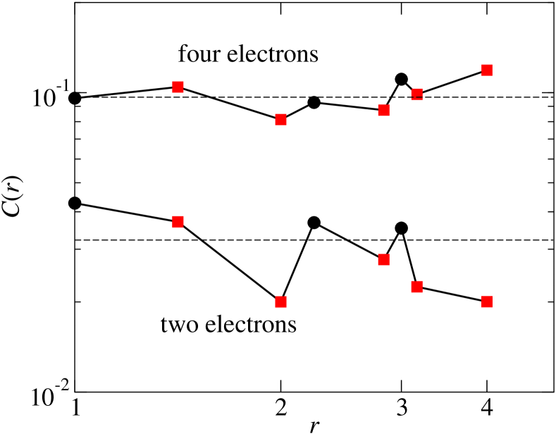
Figure 3: (Color online) Charge carrier correlation in systems doped with two and four electrons. Squares and circles indicate that the pair of electrons are in the same and opposite sublattices respectively. Dotted lines are pair correlations of uncorrelated electrons in the respective cases.

VI charge carrier correlation in momentum space

Next we go to the momentum space and study the momentum distribution function of spin objects $\langle n_{{\bf k}\sigma}\rangle=\langle\tilde{c}^{\dagger}_{{\bf k}\sigma}\tilde{c}_{{\bf k}\sigma}\rangle$. One motivation for studying $\langle n_{{\bf k}\sigma}\rangle$ is to learn about the Fermi surface of the model. For this purpose it is important to realize that in $t$-$J$-like models the momentum distribution function has a dome shape in the first Brillouin zone. This feature results from minimizing the kinetic energyew93 ; eos94 and is not related to the actual Fermi surface of the model. Nevertheless, those k points along the AFBZ boundary are not affected by this kinematic effect. Therefore it is possible to extract information on the Fermi surface from these k points. A second motivation for studying the momentum distribution function is to see whether the single-carrier ground state is relevant to the physics of the multiply-doped system. This has been a subject of discussion in the $t$-$J$ model.sh90 ; eos94 ; eo95 Note that in the electron-doped model some authors choose to report the momentum distribution function of charge carriers, $\langle{\overline{n}}_{{\bf k}\sigma}\rangle=\langle\tilde{c}_{{\bf k}\sigma}\tilde{c}^{\dagger}_{{\bf k}\sigma}\rangle$, instead of $\langle n_{{\bf k}\sigma}\rangle$. These distribution functions have the following properties:

$$\langle n_{{\bf k}\sigma}\rangle+\langle{\overline{n}}_{{\bf k}\sigma}\rangle = n^{\text{max}}_{\sigma}\equiv(N_{\sigma}+N_{c})/N,$$ (10)

$$\sum_{\bf k}\langle n_{{\bf k}\sigma}\rangle = N_{\sigma},$$ (11)

$$\sum_{\bf k}\langle{\overline{n}}_{{\bf k}\sigma}\rangle = N_{c},$$ (12)

where $N_{\sigma}$ is the number of spin objects with spin $\sigma$. In this section we will start with the single-electron momentum distribution functions. We will show that they are qualitatively similar to those in the $t$-$J$ model. Thus their features are generic to $t$-$J$-like models. We will then discuss momentum distribution functions of the two- and four-electron systems. We will show that they can be constructed from the single-carrier result and that the Fermi surfaces are consistent with small pockets at single-carrier ground state momenta.

VI.1 One-electron system

Let us begin with the one-electron ground state with $S_{z}=1/2$ and momentum $(\pi,0)$. (Note that $S_{z}$ refers to the total spin of spin objects.) The momentum distribution functions are shown in Fig. 4. We immediately notice two very prominent features that exist in both $\langle n_{{\bf k}\uparrow}\rangle$ and $\langle n_{{\bf k}\downarrow}\rangle$: (i) there exist very sharp minima at $(\pi,0)$ or $(0,\pi)$; (ii) besides these sharp minima, they are of a dome shape with a maximum around $(\pi,\pi)$ and slopes down towards a minimum at $(0,0)$.

As discussed above, the dome shape is a generic feature that also exists in the $t$-$J$ model.clg98 The only difference is that the locations of the maximum and minimum of the “dome” are interchanged compared to those in the $t$-$J$ model. This is obviously due to the opposite signs of $t$ in the two models. This dome-shape feature therefore does not represent the shape of the true Fermi surface. Note that $\langle n_{{\bf k}\uparrow}\rangle$ and $\langle n_{{\bf k}\downarrow}\rangle$ shift above and below the half-filled value of 1/2 respectively due to the restriction from Eq. (10), $\langle n_{{\bf k}\sigma}\rangle\leq n^{\text{max}}_{\sigma}$.

Similarly, sharp minima found in Fig. 4 are also found in the momentum distribution functions of the $t$-$J$ model with one hole. Just like in the $t$-$J$ model, a “dip” in $\langle n_{{\bf k}\downarrow}\rangle$ is found at the ground state momentum [$(\pi,0)$ in Fig. 4(b)], and an “antidips” in $\langle n_{{\bf k}\uparrow}\rangle$ is found at a k point which is displaced from the dip by the antiferromagnetic momentum $(\pi,\pi)$ [$(0,\pi)$ in Fig. 4(a)]. From Fig. 4(b) we find that the depth of the dip $\langle n_{{(\pi,\pi)}\downarrow}\rangle-\langle n_{{(\pi,0)}\downarrow}\rangle$ is 0.334. This is very close to $Z_{(\pi,0)}/2$ which is 0.318, indicating its close tie with the Fermi surface. Furthermore, $Z_{\bf k}$ along the edge of the AFBZ are very small. Therefore our data is consistent with a small Fermi surface, or carrier pocket, at $(\pi,0)$. This is to be expected in a lightly doped antiferromagnet.fulde Note that all features described so far are qualitatively the same in the hole- and electron-doped models. They are generic features resulting from the kinematic effect and the antiferromagnetic order of the spin background. They do not reflect the different physics of the hole- and electron-doped models.

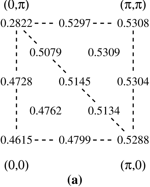
Figure 4: Momentum distribution functions (a) $\langle n_{{\bf k}\uparrow}\rangle$ and (b) $\langle n_{{\bf k}\downarrow}\rangle$ in the ground state of the one-electron system with one spin-down object removed and momentum $(\pi,0)$. Due to symmetry, only one quadrant of the Brillouin zone is shown.

VI.2 Systems with two and four electrons

When there is an even number of spin objects, $\langle n_{{\bf k}\uparrow}\rangle=\langle n_{{\bf k}\downarrow}\rangle$ and we drop the spin variable $\sigma$ from $\langle n_{{\bf k}\sigma}\rangle$. Fig. 5 shows $\langle n_{{\bf k}}\rangle$ in systems doped with two and four electrons. Again we can identity the same “dome-shape” structure found in the one-electron system. It is a generic feature of the model and does not reflect the physics of the charge carriers. Further evidence for this comes from the “height” of the dome, which is defined as $\Delta n\equiv\langle n_{(\pi,\pi)}\rangle-\langle n_{(0,0)}\rangle$. In the two-electron system it is 0.114, which is roughly the same as $\Delta n_{\uparrow}+\Delta n_{\downarrow}=0.117$ in the one-electron system. And in the four-electron system it is 0.225, roughly twice of that in the two-electron system. These agreements show that the dome-shaped structures at different doping levels are due to the same effect.

Another feature common to the one-, two- and four-electron systems is that their $\langle n_{\bf k}\rangle$ have very prominent dips at ${\bf k}=(\pi,0)$ and $(0,\pi)$. These dips resemble electron pockets. This is certainly not a generic feature of $t$-$J$-like models because it is not found in the $t$-$J$ model.clg98 Note that $(\pi,0)$ and $(0,\pi)$ are along the AFBZ boundary where $\langle n_{\bf k}\rangle$ is not disguised by the generic dome-shape feature. Therefore these pocket-like features should reflect the physics of the systems. The fact that pocket-like features are found at these doping levels immediately suggests the relevance of the singly-doped state to the multiply-doped one. If electrons doped into the parent system behave like weakly interacting fermions, then it is reasonable to expect that multiple-electron systems can be approximated by filling up the single-electron band. This should lead to electron-pockets at single-electron ground state momenta. To make this argument quantitative, we consider the charge-carrier distribution function $\langle{\overline{n}}_{\bf k}\rangle$. From Eq. (10), $\langle{\overline{n}}_{\bf k}\rangle$ can be considered as the suppression of $\langle{n}_{\bf k}\rangle$ from its maximum value upon doping. If multiple-electron states can be built up from single-electron states, we expect the suppressions in $\langle{n}_{\bf k}\rangle$ due to individual electrons doped into the system to be additive,

$$\langle{\overline{n}}_{\bf k}\rangle_{2} \simeq \langle{\overline{n}}_{{\bf k}\uparrow}\rangle_{1}+\langle{\overline{n}}_{{\bf k}\downarrow}\rangle_{1},$$

$$\langle{\overline{n}}_{\bf k}\rangle_{4} \simeq 2(\langle{\overline{n}}_{{\bf k}\uparrow}\rangle_{1}+\langle{\overline{n}}_{{\bf k}\downarrow}\rangle_{1},)$$ (13)

where $\langle{\overline{n}}_{\bf k}\rangle_{N_{c}}$ is the distribution function of a system with $N_{c}$ electrons. Table 3 shows that in the two-electron system the additive approximation is satisfied at all available k points. In the four-electron system it works satisfactorily at most k points. Obvious exceptions are $(\pi,0)$ and $(3\pi/4,\pi/4)$. Note that at this doping level Eq. (13) cannot hold at $(\pi,0)$ without violating Eq. (10). As a result, instead of filling states at $(\pi,0)$ some electrons will fill the next available low energy states which, according to Fig. 2, are at $(3\pi/4,\pi/4)$. Therefore our results show that the additive approximation works in the electron-doped model at doping levels up to at least 0.125. Note that this conclusion is consistent with that in section IV: if the electrons are uncorrelated, we expect that multiply-doped states can be build up from the singly-doped state.

Figure 5: Momentum distribution function $\langle n_{\bf k}\rangle$ in systems with (a) two and (b) four electrons.

Table 3: Charge-carrier distribution function $\langle{\overline{n}}_{\bf k}\rangle$ in systems doped with two and four electrons. Numbers in brackets are the corresponding results from the additive approximation Eq. (13). Note that in Eq. (13) we have to average the one-carrier results over all degenerate ground states.

k	two-electron system	four-electron system
(0,0)	0.1150 (0.1179)	0.2280 (0.2357)
($\frac{\pi}{4}$,$\frac{\pi}{4}$)	0.0935 (0.0941)	0.2002 (0.1882)
($\frac{\pi}{2}$,$\frac{\pi}{2}$)	0.0304 (0.0301)	0.0614 (0.0602)
($\frac{3\pi}{4}$,$\frac{3\pi}{4}$)	0.0008 (0.0009)	0.0021 (0.0018)
($\pi$,$\pi$)	0.0006 (0.0008)	0.0027 (0.0015)
($\pi$,$\frac{\pi}{2}$)	0.0024 (0.0021)	0.0051 (0.0042)
($\pi$,0)	0.3574 (0.3550)	0.3901 (0.7099)
($\frac{\pi}{2}$,0)	0.0932 (0.0928)	0.2108 (0.1855)
($\frac{3\pi}{4}$,$\frac{\pi}{4}$)	0.0361 (0.0362)	0.1338 (0.0724)

VII Spin order

Our previous discussions have been based on the scenario that antiferromagnetic spin order is preserved upon doping. This is a direct consequence of the fact that the $t^{\prime}$ and $t^{\prime\prime}$ hopping terms do not frustrate the spin background. In this section we provide evidence for the existence of antiferromagnetic correlation. Antiferromagnetic spin order can be measured directly using the spin correlation function $\langle{\bf S}_{0}\cdot{\bf S}_{r}\rangle$. Results are shown in Fig. 6(a). At half-filling the system is known to possess long-range antiferromagnetic orderm91 and its spin correlation is shown as a reference. We note that in the two-electron system the spin correlation is not much weaker than that at half-filling, and more importantly it does not show significant decay beyond $r=\sqrt{2}$. This indicates that strong antiferromagnetic spin order exists in the system. The same qualitative trend is also observed in the four-electron system. Although the spin correlation is inevitably weakened due to higher doping level, it does not decay significantly beyond $r=\sqrt{2}$. Another way to display the same data is through the static structure factor,

$$S({\bf k})=\sum_{r}e^{i{\bf k}\cdot{\bf r}}\langle{\bf S}_{0}\cdot{\bf S}_{r}\rangle.$$ (14)

Fig. 6(b) shows the structure factors in systems doped with two and four electrons. As the doping level increases, the height of the antiferromagnetic peak at $(\pi,\pi)$ is reduced. But it still remains prominent and there is no sign of enhancement at any other k point. Our results therefore indicate that antiferromagnetic order persists at least up to $x=0.125$. Note that this doping level is close to the point where the antiferromagnetic phase ends in the phase diagram of NdCeCuO,d94 which is $x=0.13$.

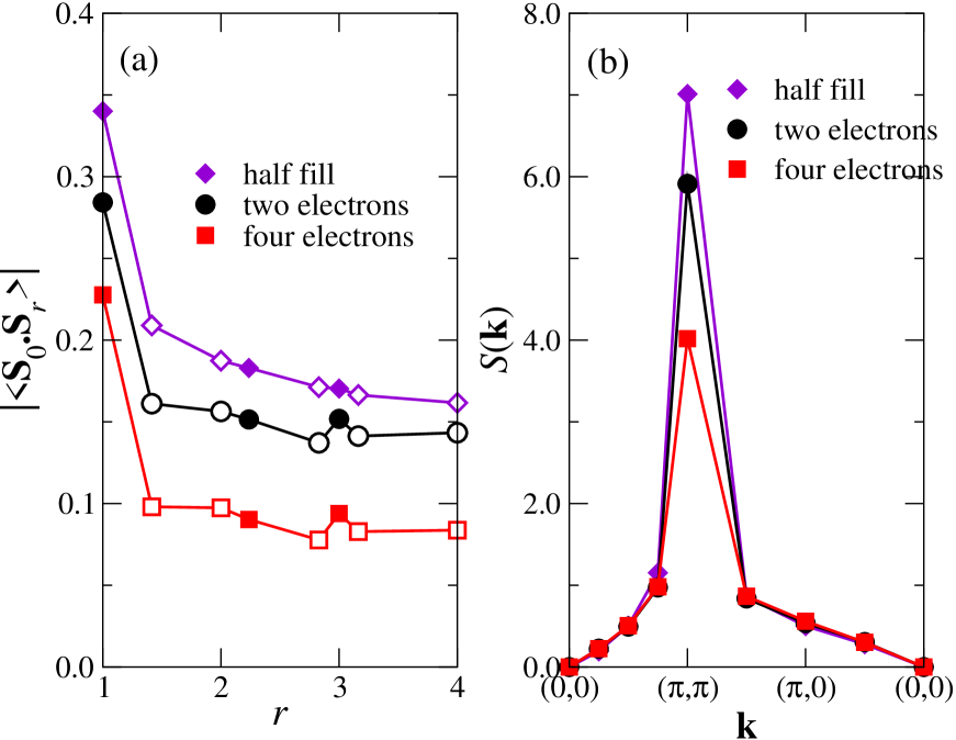
Figure 6: (Color online) (a) Spin correlation function and (b) static structure factor of systems with two and four electrons. Results at half-filling are given for reference purpose. In (a), empty and filled symbols represent positive and negative correlations respectively.

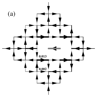
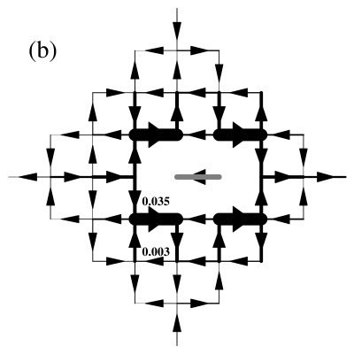
Figure 7: Current correlation $\langle j_{kl}j_{mn}\rangle/x$ in the ground state of the (a) two-electron, and (b) four-electron systems. The reference bond $mn$ is indicated by a shaded line. On other bonds, arrows point along the directions of positive correlation and line widths are proportional to $\langle j_{kl}j_{mn}\rangle/x$. For reference purpose, numerical values of $\langle j_{kl}j_{mn}\rangle/x$ are shown next to some of the bonds.

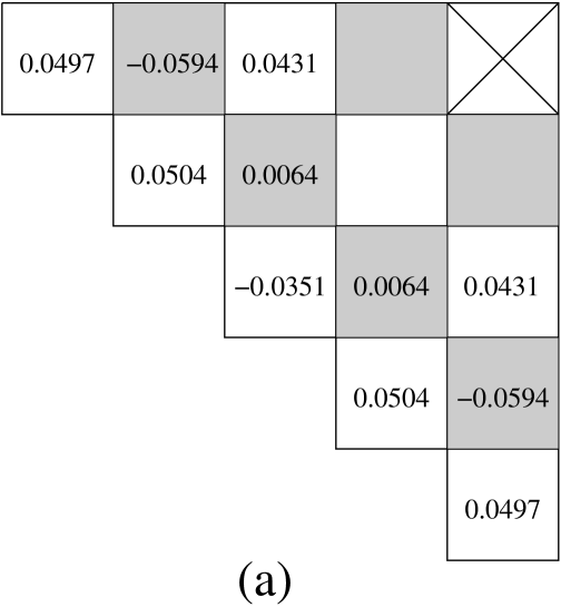
Figure 8: Vorticity correlation $C_{VV}(r)$ in the ground state of the (a) two-electron and (b) four-electron systems. The reference plaquette is indicated by a cross inside it. Those plaquettes touching the reference one do not have well-defined vorticity correlation because current operators on overlapping bonds do not commute.

VIII Charge current correlation

The existence of a staggered pattern in the charge current correlation function has been established in the $t$-$J$ model.ilw00 ; l00 It has been interpreted as a direct evidence for the staggered-flux phase in the mean-field picture.we01 In this picture the hopping motions of charge carriers frustrate the antiferromagnetic spin background and lead to staggered chiral spin correlation. Binding of charge carriers is mediated through the attraction between charge carriers with opposite vorticity. Numerically it has been found that staggered current pattern exists in the two-hole $t$-$J$ model with $d_{x^{2}-y^{2}}$ symmetry only when the holes are loosely bound. It does not exist in states with other symmetry, nor when $J/t$ is so large that the holes are tightly bound. The vorticity and charge correlations are found to be proportional to each other. However, in the electron-doped model a very basic ingredient of the above picture is missing, namely, the hopping motions of charge carriers are mostly unfrustrating. The result is that antiferromagnetic order is robust and charge carriers do not have significant correlation. Consequently it is very unlikely that staggered current correlation can exist. However, as antiferromagnetic spin order is weakened at higher doping level, more subtle correlations may emerge.rw03 We therefore calculate the current correlation in the two- and four-carrier ground states and see if there exists a systematic trend as doping level increases.

Fig. 7 shows the spatial variation of the current correlation function $\langle j_{kl}j_{mn}\rangle$, where

$$j_{kl}=i(\tilde{c}^{\dagger}_{k}\tilde{c}_{l}-\tilde{c}^{\dagger}_{l}\tilde{c}_{k}),$$ (15)

for systems doped with two and four electrons. Another way to display the same data is to define the vorticity $V({\bf r})$ of a square plaquette by summing up the current around it in the counterclockwise direction. The vorticity correlation $C_{VV}(r)\equiv\langle V(r)V(0)\rangle/x$ is shown in Fig. 8. Our result for the two-electron system leaves little doubt that there is no staggered pattern in either $\langle j_{kl}j_{mn}\rangle$ or $C_{VV}(r)$. In the four-electron system there is again no clear indication of a staggered pattern. We therefore conclude that intra-sublattice hopping terms in the electron-doped model do not favor the formation of a staggered pattern in the current correlation. This agrees with a recent mean-field study on the electron-doped model.rw03 Furthermore, in the mean-field picture the loss of vorticity correlation implies that charge carrier binding is not favored, which agrees with our results in section V. Finally we remark that in our four-electron system, it seems like at short distances the current correlation is stronger and exhibit a staggered pattern. This is most obvious when we compare Fig. 8(a) and (b). This seems to suggest that at doping level $x=0.125$ the system may be starting to develop some other order due to the weakening of antiferromagnetic correlation. However, the range within which we observe the “right” correlation is too short and the correlation is too weak for us to decide whether it has any significance. Therefore we are not able to make any definite statement concerning this matter.

IX Conclusion

We have solved the electron-doped model with one, two, and four charge carriers on a 32-site square lattice. Our results cover doping levels up to $x=0.125$. In the electron-doped model, intra-sublattice hoppings of charge carriers do not frustrate the spin background. Most of our results presented above can be understood as consequences of this fact. Since hopping motions are mostly unfrustrating, charge carriers can propagate more freely. This is reflected in the large quasi-particle bandwidth in the singly-doped system. In systems doped with two and four electrons, the charge carrier correlation function shows that electrons are uncorrelated. Again this is due to the fact that electrons can hop more freely in the same sublattice. There is no evidence of charge carriers forming a bound state. Unfrustrating hopping motions also mean that antiferromagnetic correlation in the spin background is better preserved upon doping. This is clearly shown in the spin correlation function and static structure factor. It also shows up in the Fermi surface of the system. In the singly-doped system quasi-particle weights at k points along the AFBZ boundary are small except at the single-carrier ground state momenta, i.e., $(\pi,0)$ and its equivalent points. This resembles a Fermi surface consisting of small pockets at single-carrier ground state momenta, which is expected in a lightly doped antiferromagnet.fulde These small pockets persist in our systems doped with two and four electrons and are clearly visible in their momentum distribution functions of spin objects. Furthermore, momentum distribution functions of our multiply-doped systems can be well approximated by adding up the singly-doped momentum distribution functions. This re-assures that charge carriers are uncorrelated.

Our results show that antiferromagnetic order in electron-doped model persists at least up to doping level $x=0.125$. We find no clear evidence of other orders existing in our systems. This is consistent with the phase diagram of $\text{Nd}_{2-x}\text{Ce}_{x}\text{CuO}_{4}$ whose antiferromagnetic phase persists up to $x=0.13$.d94 ARPES experiment on the same material shows that before the Fermi surface becomes a large one centered at $(\pi,\pi)$, small pockets will start to appear at $(\pi/2,\pi/2)$ (and its equivalent points) as those at $(\pi,0)$ evolve.dhs03 However, the quasi-particle energy $E({\bf k})$ at ${\bf k}=(\pi/2,\pi/2)$ in the electron-doped model is quite high (see Fig. 2). Assuming that the quasi-particle dispersion relation does not change much on further doping, electrons doped into the system will fill lower energy states at other k points first. Therefore it is not surprising that we do not see pockets developing at $(\pi/2,\pi/2)$. A recent theoretical calculation predicts that pockets will start to appear at $(\pi/2,\pi/2)$ at $x=0.144$ when the Fermi level crosses a different band from that at lower doping levels.yclt04 Therefore it is possible that our doping level is not large enough to observe the change in the Fermi surface as revealed by ARPES experiment.

- (1) E. Dagotto, Rev. Mod. Phys. 66, 763 (1994).
- (2) T. Tohyama and S. Maekawa, Phys. Rev. B 49, 3596 (1994).
- (3) R. J. Gooding, K. J. E. Vos, and P. W. Leung, Phys. Rev. B 50, 12866 (1994).
- (4) N. P. Armitage, F. Ronning, D. H. Lu, C. Kim, A. Damascelli, K. M. Shen, D. L. Feng, H. Eisaki, Z.-X. Shen, P. K. Mang, N. Kaneko, M. Greven, Y. Onose, Y. Taguchi, and Y. Tokura, Phys. Rev. Lett. 88, 257001 (2002).
- (5) A. Damascelli, Z. Hussain, and Z.-X. Shen, Rev. Mod. Phys. 75, 473 (2003).
- (6) T. Tohyama and S. Maekawa, Phys. Rev. B 64, 212505 (2001).
- (7) T. Tohyama and S. Maekawa, Phys. Rev. B 67, 92509 (2003).
- (8) T. Tohyama, Phys. Rev. B 70, 174517 (2004).
- (9) Q. Yuan, Y. Chen, T. K. Lee, and C. S. Ting, Phys. Rev. B 69, 214523 (2004).
- (10) Q. Yuan, T. K. Lee, and C. S. Ting, Phys. Rev. B 71, 134522 (2005).
- (11) We remark that there is another approach to the electron-doped model which, in contrast to the strong coupling limit assumed in the - model, emphasizes the importance of intermediate coupling. See, for example, D. Sénéchal and A.-M. S. Tremblay, Phys. Rev. Lett. 92, 126401 (2004), and references there-in.
- (12) P. W. Leung and R. J. Gooding, Phys. Rev. B 52, R15711 (1995).
- (13) A. L. Chernyshev, P. W. Leung, and R. J. Gooding, Phys. Rev. B 58, 13594 (1998).
- (14) P. W. Leung, Phys. Rev. B 65, 205101 (2002).
- (15) P. W. Leung, cond-mat/0511568.
- (16) P. W. Leung and K. K. Ng, Int. J. Mod. Phys. B 17, 3367 (2003).
- (17) P. W. Leung, B. O. Wells, and R. J. Gooding, Phys. Rev. B 56, 6320 (1997).
- (18) It has been suggested that in the electron-doped model not only the signs and the magnitudes of the hopping terms are different from those in the hole-doped model (see Ref. eskes, ). But since we are not interested in the detail quantitative differences, we only change the signs of the hopping terms in the electron-doped model.
- (19) Note that in the electron-doped model this definition of corresponds to inverse photoemission spectroscopy on the undoped insulator. A similar definition in the - model corresponds to photoemission spectroscopy, see Ref. lwg97, .
- (20) V. I. Belinicher, A. L. Chernyshev, and V. A. Shubin, Phys. Rev. B 53, 335 (1996).
- (21) J. A. Riera and A. P. Young, Phys. Rev. B 39, R9697 (1989).
- (22) R. Eder and P. Wróbel, Phys. Rev. B 47, 6010 (1993).
- (23) R. Eder, Y. Ohta, T. Shimozato, Phys. Rev. B 50, 3350 (1994).
- (24) W. Stephan and P. Horsch, Phys. Rev. Lett. 66, 2258 (1990).
- (25) R. Eder and Y. Ohta, Phys. Rev. B 51, 6041 (1995).
- (26) P. Fulde, Electron Correlations in Molecules and Solids, edition, (Springer, Berlin, 1995).
- (27) E. Manousakis, Rev. Mod. Phys. 63, 1 (1991).
- (28) D. A. Ivanov, P. A. Lee, and X.-G. Wen, Phys. Rev. Lett. 84, 3958 (2000).
- (29) P. W. Leung, Phys. Rev. B 62, R6112 (2000).
- (30) We remark that there is another independent interpretation of the same result in the spin-polaron picture. See P. Wróbel and R. Eder, Phys. Rev. B 64, 184504 (2001).
- (31) T. C. Ribeiro and X.-G. Wen, Phys. Rev. B 68, 24501 (2003).
- (32) H. Eskes and G. A. Sawatzky, Physica C 160, 424, (1989).