Morphologies and flow patterns in quenching of lamellar systems with shear

Abstract

We study the behavior of a fluid quenched from the disordered into the lamellar phase under the action of a shear flow. The dynamics of the system is described by Navier-Stokes and convection-diffusion equations with pressure tensor and chemical potential derived by the Brazovskii free-energy. Our simulations are based on a mixed numerical method with Lattice Boltzmann equation and finite difference scheme for Navier-Stokes and order parameter equations, respectively. We focus on cases where banded flows are observed with two different slopes for the component of velocity in the direction of the applied flow. Close to the walls the system reaches a lamellar order with very few defects and the slope of the horizontal velocity is higher than the imposed shear rate. In the middle of the system the local shear rate is lower than the imposed one and the system looks as a mixture of tilted lamellae, droplets and small elongated domains. We refer to this as to a region with a Shear Induced Structures (SIS) configuration. The local behavior of the stress shows that the system with the coexisting lamellar and SIS regions is in mechanical equilibrium. This phenomenon occurs, at fixed viscosity, for shear rates under a certain threshold; when the imposed shear rate is sufficiently large, lamellar order develops in the whole system. Effects of different viscosities have been also considered: The SIS region is observed only at low enough viscosity. We compare the above scenario with the usual one of shear banding. In particular, we do not find evidence for a plateau of the stress at varying imposed shear rates in the region with banded flow. We interpret our results as due to a tendency of the lamellar system to oppose to the presence of the applied flow.

I Introduction

Complex fluids such as polymer solutions, liquid crystals, or surfactant systems are characterized by the presence of organized structures at mesoscopic scales between macroscopic and solvent molecular lengths CE . Under the action of external forcing, the coupling between the mesoscopic structures and the local velocity field makes the flow properties of complex fluids different from those of simple liquids larson . For example, when a shear flow is applied to a simple fluid, after a short initial transient, the linear relation between the stress $S$ and the shear rate $\gamma$ is verified, $S=\eta\gamma$ with $\eta$ being the fluid viscosity. In complex fluid an effective viscosity can be defined by the same relation but its value is not constant, depending on the strength of the applied flow. In systems with interfaces, for examples, the effective viscosity generally decreases (shear thinning) when the shear rate is increased due to the alignment of interfaces with the flow.

In some cases the flow can induce new organization in the fluid BRP94 . In lamellar phases, for instance, onion and hexagonal phases have been observed not existing at rest CBDCL ; HBP ; PAR . Such shear induced structures (SIS) can coexist in a range of applied shear rates with the structures unmodified by the flow. Usually the SIS and the unmodified phase have different viscosities so that they flow with different profiles. This phenomenon, called shear banding, has been observed in many complex fluids and also in lamellar systems RND ; SCM . Its microscopic origin is not yet completely understood and different explanations have been proposed depending on the system Olmstedrev .

The traditional theoretical description of shear banding and other rheological behaviors in complex fluids is based on the assumption of a local relation between the stress and the shear rate EYB ; olm99 . However, in this way, the role of the structures present in the fluid is not evident and they cannot be directly related to the flow pattern. While a full description of the system with all its molecular dynamical variables is not possible, a description at mesoscopic level based on an order parameter evolution equation can enlighten many issues concerning the kinetics of shear banding, the morphology of the different structures in the fluid and the evolution of the flow field Onuki97 ; Yeomans . Since the formation of SIS often occurs during transient regimes and since, also under stationary conditions, the flow pattern is not known a priori, one understands that a description based on both Navier-Stokes and order parameter equations is generally required. The hydrodynamical description is useful also for comparisons with experiments where not always the dynamical quantities are all easily accessible.

The aim of this paper is twofold. First, we want to show the relevance of the full hydrodynamical description also in systems with applied flow and see how a specific problem can be conveniently studied by our simulation methods. Then we hope to clarify some aspects of the kinetics of formation of lamellar phases in cases when banded flows are observed olm03 . In our model the lamellar properties are encoded in a free-energy functional of an order parameter representing the relative concentrations of substances in the mixture. The order parameter follows a convection-diffusion equation; from its instantaneous configurations the stress can be calculated and inserted in the Navier-Stokes equation without assuming a further stress-shear rate constitutive relation.

The free-energy functional considered in this paper was originally introduced to study the effects of fluctuations in the disordered-lamellar phase transition B75 and later used to describe equilibrium properties of di-block copolymer systems Lei80 . Solutions of copolymers, consisting of A-polymers covalently bonded to B-polymers in pairs, can organize in striped phases where A-rich and B-regions are separated by a stack of lamellae Bat . The order parameter in this case represents the relative concentration of A and B substances. Our model is also relevant for other systems with lamellar order. We mention ternary mixtures where the surfactant form interfaces between oil and water GS94 , dipolar SD and supercooled liquids KKZNT95 , chemically reactive binary mixtures GC .

The dynamical equations will be solved using a numerical scheme based on a Lattice Boltzmann Method (LBM) for the Navier-Stokes equation and finite difference methods for the convection-diffusion equation. LBM solves numerically a minimal Boltzmann equation where the fluid can only move along the links of a regular lattice with dynamics consisting of a free-streaming and a collision step lbe-1 . LBM has been largely applied to the study of binary mixtures and complex flows Yeomans ; Swift96 ; yeo ; noishear ; lbe-2 . Rheological behavior of liquid crystals under shear has been studied by LBM in Ref. DOY . The mixed method used in this paper luo ; Xuepl ; noidsfd allows a reduction in memory which is convenient in large scale simulations. Moreover, spurious terms appearing in Eq. (8) Swift96 are avoided and the numerical efficiency is increased.

In our simulations we start from a disordered configuration and consider the evolution of the system with parameters corresponding to the lamellar phase. This correspond to a sudden quench; shear is applied for all the evolution after the quench. Lamellae are expected to align with the flow with order propagating from the moving walls tanaka . One could think that after a sufficient long time lamellae will be ordered uniformly in the whole system. However, we will see that the system can behave differently. In some range of parameters we will find that a SIS region develops in the middle of the system consisting of small droplets and pieces of bent and rolled lamellae. This region coexists with lamellar regions close to the walls and a banded flow with different shear rates is observed. These results will be discussed in relation with the traditional scenario of shear banding EYB ; olm99 ; olmsted .

The paper is organized as follows. In the next Section the equilibrium model and the dynamical equations will be first introduced. Then the various components of the stress and the structure factor will be defined. Finally, a short review of the numerical scheme we use will be given. Section III contains our results for the evolution of the system in a specific case where a SIS region with banded flow is observed. The effects of changing viscosity and shear rate on the properties of the SIS region will be shown in Section IV. In Section V we analyze the evolution of global order in the system in the spirit of what usually done in phase separation studies, considering the behavior of the first momenta of the structure factor. A discussion with conclusions will be given in Section VI.

II The model and the method

Our simulations are based on a mixed numerical approach which combines the lattice Boltzmann method with a finite difference scheme Xuepl ; noidsfd . In this scheme the equilibrium properties of the system can be controlled by introducing a free energy.

II.1 Equilibrium properties and dynamical equations

The equilibrium phase is described by a coarse grained free energy that, for the specific problem we study here, is the following:

$$F\!=\!\int d{\bf r}\left[\frac{1}{3}n\ln n+\frac{a}{2}\varphi^{2}+\frac{b}{4}\varphi^{4}+\frac{\kappa}{2}(\nabla\varphi)^{2}+\frac{d}{2}(\nabla^{2}\varphi)^{2}\right]$$ (1)

where $n$ is the total density of the system and $\varphi$ is a scalar order parameter representing the concentration difference between the two components of the mixture. The term in $n$ gives rise to a positive background pressure and does not affect the phase behavior. The terms in $\varphi$ correspond to the Brazovskii free energy B75 . We take $b,d>0$ to ensure stability. For $a>0$ the fluid is disordered; for $a<0$ and $\kappa>0$ two homogeneous phases with $\varphi=\pm\sqrt{-a/b}$ coexist. A negative $\kappa$ favors the presence of interfaces and a transition into a lamellar phase can occur. In single mode approximation, assuming a profile like $A\sin k_{0}x$ for the direction transversal to the lamellae, one finds the transition ($|a|=b$) at $a\approx-1.11\kappa^{2}/d$ where $k_{0}=\sqrt{-\kappa/2d}$ and $A^{2}=4(1+\kappa^{2}/4db)/3$ Xuepl .

The evolution of the system is described by a set of two coupled partial differential equations: The Navier-Stokes and the convection-diffusion equations. The fluid local velocity ${\bf u}$ obeys, by assuming incompressibility (${\bf\nabla}\cdot{\bf u}=0$), the Navier-Stokes equation which reads as

$$n\Big{(}\partial_{t}u_{\alpha}+{\bf u}\cdot{\bf\nabla}u_{\alpha}\Big{)}=-\partial_{\beta}P_{\alpha\beta}^{th}+n\nu\nabla^{2}u_{\alpha}\;\;\;\;,$$ (2)

where $\nu$ is the kinematic viscosity. $P_{\alpha\beta}^{th}$ is the thermodynamic pressure tensor which can be calculated from the free energy functional (1) as

$$P_{\alpha\beta}^{th}=\Big{\{}n\frac{\delta F}{\delta n}+\varphi\frac{\delta F}{\delta\varphi}-f(n,\varphi)\Big{\}}\delta_{\alpha\beta}+D_{\alpha\beta}(\varphi)$$ (3)

where $f(n,\varphi)$ is the free-energy density and a symmetric tensor $D_{\alpha\beta}(\varphi)$ has to be added to ensure that the condition of mechanical equilibrium $\partial_{\alpha}P_{\alpha\beta}^{th}=0$ is satisfied evans . The complete expression of the pressure tensor is yeo

$$P_{\alpha\beta}^{th}=p\delta_{\alpha\beta}+P_{\alpha\beta}^{chem}$$ (4)

with

$$p=\frac{1}{3}n+\frac{a}{2}\varphi^{2}+\frac{3b}{4}\varphi^{4}-\kappa\big{[}\varphi(\nabla^{2}\varphi)+\frac{1}{2}(\nabla\varphi)^{2}\big{]}$$

$$+d\big{[}\varphi(\nabla^{2})^{2}\varphi+\frac{1}{2}(\nabla^{2}\varphi)^{2}+\partial_{\gamma}\varphi\partial_{\gamma}(\nabla^{2}\varphi)\big{]}$$ (5)

and

$$P_{\alpha\beta}^{chem}=\kappa\partial_{\alpha}\varphi\partial_{\beta}\varphi-d\big{[}\partial_{\alpha}\varphi\partial_{\beta}(\nabla^{2}\varphi)+\partial_{\beta}\varphi\partial_{\alpha}(\nabla^{2}\varphi)\big{]}$$ (6)

Moreover, we shear the system by moving the upper and lower walls with velocities

$${\bf v}_{u,l}=\pm\gamma\frac{L}{2}{\bf i},$$ (7)

respectively, where $\gamma$ is the shear rate, $L$ is the width of the system and ${\bf i}$ is a unit vector along the $x$-axis, which is usually denoted as the flow direction. The presence of the moving walls greatly affects, as we will see, the fluid velocity ${\bf u}$ and the behavior of the order parameter $\varphi$.

The evolution of $\varphi$ is described by the convection-diffusion equation:

$$\partial_{t}\varphi+{\bf\nabla}\cdot(\varphi{\bf u})=\Gamma\nabla^{2}\mu$$ (8)

where

$$\mu=\frac{\delta F}{\delta\varphi}=a\varphi+b\varphi^{3}-\kappa\nabla^{2}\varphi+d(\nabla^{2})^{2}\varphi$$ (9)

is the chemical potential footnote , $\Gamma$ is a mobility coefficient, and the laplacian in the r.h.s. of (8) guarantees the conservation of $\varphi$.

II.2 The shear stress

The presence of shear strongly influences the morphology of the system and its rheological properties. In particular, we will consider the effects on shear stress.

The total stress is (see the r.h.s. of Eq. (2))

$$S_{\alpha\beta}=-P_{\alpha\beta}^{th}+n\nu\left(\partial_{\beta}u_{\alpha}+\partial_{\alpha}u_{\beta}\right).$$ (10)

The total shear stress, which is related to the off-diagonal part of the total stress (10) larson , is

$$S_{xy}=-P_{xy}^{chem}+n\nu\left(\partial_{y}u_{x}+\partial_{x}u_{y}\right)$$ (11)

$S_{xy}$ is the sum of the time reversible shear stress $S_{xy}^{chem}=-P_{xy}^{chem}$ and of a dissipative hydrodynamic contribution $S_{xy}^{hydr}=n\nu(\partial_{y}u_{x}+\partial_{x}u_{y})$. The expression (11) depends on local coordinates and may vary from point to point especially when the system is not homogeneous.

A quantity of relevant experimental interest is the integral

$$S=\int d{\bf r}S_{xy}=S^{chem}+S^{hydr}=\int d{\bf r}S_{xy}^{chem}+\int d{\bf r}S_{xy}^{hydr}$$ (12)

By using Eq. (6) it can be shown that $S^{chem}$ can be also calculated in the reciprocal space as

$$S^{chem}=\int d{\bf r}S_{xy}^{chem}=\int\frac{d{\bf k}}{(2\pi)^{d}}k_{x}k_{y}(\kappa+2dk^{2})C({\bf k},t),$$ (13)

where $C({\bf k},t)$ is the structure factor

$$C({\bf k},t)=\langle\varphi({\bf k},t)\varphi(-{\bf k},t)\rangle,\qquad$$ (14)

$\varphi({\bf k})$ is the Fourier transform of the order parameter $\varphi$ and $\langle\cdot\rangle$ is the average over different histories.

II.3 The numerical scheme

The Eqs. (2-8) are numerically solved in 2D by using a mixed approach. We use the lattice Boltzmann method for Eq. (2) and a finite difference scheme for Eq. (8). Such an approach has been already adopted in the case of thermal lattice Boltzmann models for a single fluid and for multiphase flows luo . In that case it is the temperature equation to be solved by finite differences. By using this approach we are able to avoid the spurious terms in the convection-diffusion equation (8) which come into play when standard LBM for binary mixtures is used Swift96 , though LBM may realize boundary conditions easily and give better numerical stability. The present method allows to reduce required memory.

A set of distribution functions $f_{i}({\bf r},t)$ is defined on each lattice site ${\bf r}$ at each time $t$. Each function is associated to a lattice speed vector ${\bf e}_{i}$ with $e_{i}/c=$ $(\pm 1,0),(0,\pm 1),(\pm 1,\pm 1),(0,0)$, where $c=\Delta x/\Delta t$, $\Delta t$ is the time step, and $\Delta x$ is the lattice constant.

They evolve according to a single relaxation-time Boltzmann equation bhat ; lbe-1 :

$$f_{i}({\bf r}+{\bf e}_{i}\Delta t,t+\Delta t)-f_{i}({\bf r},t)=-\frac{1}{\tau}[f_{i}({\bf r},t)-f_{i}^{eq}({\bf r},t)]$$ (15)

where $\tau$ is a relaxation parameter and $f_{i}^{eq}({\bf r},t)$ are local equilibrium distribution functions. They are related to the total density $n$ and to the fluid momentum $n{\bf u}$ through

$$n=\sum_{i}f_{i},\;\;\;\;n{\bf u}=\sum_{i}f_{i}{\bf e}_{i}.$$ (16)

These quantities are locally conserved in any collision process and, therefore, we require that the local equilibrium distribution functions fulfil the equations

$$\sum_{i}f_{i}^{eq}=n,\;\;\;\;\sum_{i}f_{i}^{eq}{\bf e}_{i}=n{\bf u}.$$ (17)

Following Ref. Swift96 , the higher moments of the local equilibrium distribution functions are defined so that the Navier-Stokes equation can be obtained and the equilibrium thermodynamic properties of the system can be controlled:

$$\sum_{i}f_{i}^{eq}e_{i\alpha}e_{i\beta}=c^{2}P_{\alpha\beta}^{th}+nu_{\alpha}u_{\beta}.$$ (18)

The local equilibrium distribution functions can be expressed as an expansion at the second order in the velocity ${\bf u}$ Swift96 . The expression of the coefficients of the equilibrium distribution functions can be found in Ref. noi .

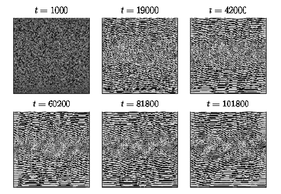
Figure 1: Configurations of the order parameter $\varphi$ on the whole $1024\times 1024$ lattice for the case with $\gamma=5\times 10^{-5}$ and $\nu=4.1667$.

The above described lattice Boltzmann scheme simulates at second order in $\Delta t$ the continuity and the incompressible Navier-Stokes equations (2) with the kinematic viscosity $\nu$ given by

$$\nu=\Delta t\frac{c^{2}}{3}(\tau-\frac{1}{2}).$$ (19)

It appears that the relaxation parameter $\tau$ can be used to tune independently the viscosity.

Equation (8) is numerically integrated by using an explicit Euler scheme on a square lattice with spacing $\Delta x$, the same as for LBM. The spatial derivatives are approximated by discrete expressions which are second order in $\Delta x$. The time step is $\Delta t^{\prime}=\Delta t/m$ with $m=5$. This choice was motivated by the observation of a better numerical stability of the code.

To enforce the flow (7) we assume periodic boundary conditions (BC) along the flow direction and we place walls at the upper and lower rows of the lattice moving them at a constant velocity along the $x$ direction avoiding slip velocity noishear . The velocity ${\bf u}$ obtained from Eq. (16) goes inside the convection-diffusion equation (8). For the order parameter $\varphi$ we adopt Lees-Edwards BC along the $y$ direction lees . This means that $\varphi(x,-L/2)=\varphi(x+(v_{u}-v_{l})\Delta t^{\prime},L/2)$. The algorithm implementing the previous numerical scheme has been described in Ref. noidsfd .

All the simulations in the following have been run by using the parameters $-a=b=2\times 10^{-4}$, $\kappa=-6\times 10^{-4}$, $d=7.6\times 10^{-4}$, and $\Gamma=25$. The system size was $L=1024$ and space and time steps were set to $\Delta x=1$ and $\Delta t=0.2$, respectively. At the beginning of each run the values of $\varphi$ are randomly taken in the range $[-0.1,0.1]$, the distribution functions $f_{i}$ are set so that $n=1$, and the velocities ${\bf u}$ are computed from Eq. (16). We verified that by vertically shifting the reference frame, the fluid velocity profile is accordingly shifted. Therefore we used the choice of placing the walls symmetrically located at $y=\pm L/2$ to have fluid almost at rest in the middle of the system.

III Kinetics of SIS formation

In this Section we will show the evolution of the system described by Eqs. (2,8) for a typical case where shear induced structures appear. Shear rate and viscosity are fixed to $\gamma=5\times 10^{-5}$ and $\nu=4.1667$. All the quantities here and in the following are measured in units of the space step $\Delta x$ and the time step $\Delta t$. For these values, the relaxation time of the linear shear velocity profile in a simple fluid would be of the order of $t=6000$ footnote2 .

Figure 1 shows the configurations of $\varphi$ at successive times. At $t=1000$ after the quench, the order parameter has locally reached one of the minima of the polynomial part of the free-energy, represented by black and white in the figure. Lamellae are ordered only on small scales and in most of the system the effects of shear flow are not observable. Ordered structures appear only very close to the walls. At the next time $t=19000$, lamellar order has developed into the system, but the the middle region is still almost isotropic apparently scarcely influenced by the flow. After this time the region of lamellae aligned with the flow does not increase the extension towards the central part of the system where morphology evolves in a different way. At $t=42000$ the middle region mostly consists of lamellae oriented at about $45^{o}$ with respect to the direction of the flow. Few domains are broken into droplets and small pieces of lamellae. The interface between the central and the two external lamellar regions is not very sharp and shows some undulations.

The further evolution of the middle region can be seen at $t=60200$. We will call this region as a SIS region or SIS phase. Many ruptures have occurred in the central network with the consequent formation of more droplets and worm-like domains. Not relevant changes can be observed at $t=81800$ and $t=101800$. Droplets, once formed, are quite stable. We checked the existence of the SIS region until time $t=200000$. We repeated this numerical experiment starting from 5 different initial configurations and obtaining very similar results for the different histories.

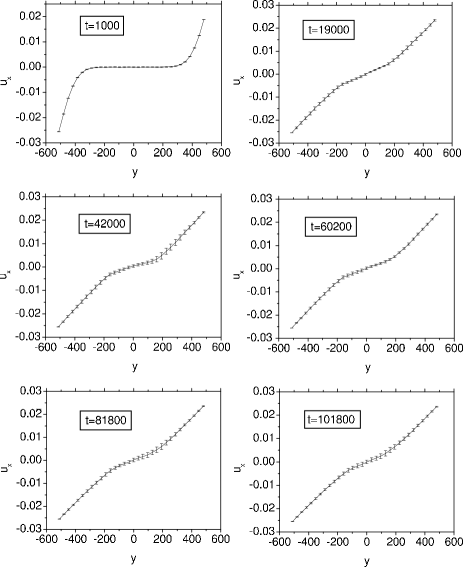
Figure 2: Plots of the $x$-averaged horizontal velocities across the system at different times for the case with $\gamma=5\times 10^{-5}$ and $\nu=4.1667$.

The morphological evolution of the system has to be examined also in relation with the behavior of the velocity profile. In Fig. 2 the $x$-averaged horizontal velocities $u_{x}$ are plotted at the same times of Fig. 1 a functions of $y$. The variance corresponding to each average is also shown; it is generally quite small indicating an uniform behavior of the system in the flow direction. At the beginning ($t=1000$) the shear profile is different from zero only in a region of about $150$ lattice sizes close to the walls; this explains the isotropy of the configuration observed almost everywhere at this time in Fig. 1. At later times the $u_{x}$-profile becomes characterized by two slopes found in correspondence of the regions with lamellar and SIS phases. The profile remains almost stationary from $t\sim 40000$; the local shear rates in the lamellar and SIS regions are respectively higher and lower than the imposed value.

Figure 3: Plots of the different components of stress, summed over the $x$-axis, as functions of time at different positions across the system for the case with $\gamma=5\times 10^{-5}$ and $\nu=4.1667$.

Mechanical properties are described by the behavior of the two stress $S_{xy}^{chem}$ and $S_{xy}^{hydr}$. The structures present in the system locally determine the value of the chemical part of the stress. $S_{xy}^{chem}$ is larger in presence of defects or configurations which are not minima of the free-energy while it is close to zero for a well ordered lamellar configuration. This can be seen in the central part of Fig. 3 where we compare the chemical stress at different distances from the walls. In the middle of the system ($y=0$) the $x$-averaged stress reaches a maximum in correspondence of the formation of the SIS and then remains different from zero. Fluctuations correspond to the evolution of structures present in the SIS phase. The behavior of the chemical stress at $y=L/8$, just inside the SIS region, is similar. On the other hand, in the region with lamellar order, at $y=L/4$ and $y=3L/8$, after a maximum at initial times, the stress relaxes to a very small value. This maximum occurs before than lamellae become aligned with the flow. This behavior is analogous to that observed in phase separation of binary mixtures under shear where the excess viscosity reaches a maximum before than domains orientate with interfaces in the direction of the flow giapp .

The hydrodynamical stress, also shown in Fig. 3, has an opposite behavior: It is larger where shear rate is larger ($y=L/4$ and $y=3L/8$). Closer to the walls ($y=3L/8$) it relaxes to a constant value after an initial maximum corresponding to the fact that the shear rate close to the walls is higher at initial times. The bottom part of Fig. 3 shows that the system is in mechanical equilibrium from $t\sim 20000$ onwards when the total stress has become the same at different distances from the walls.

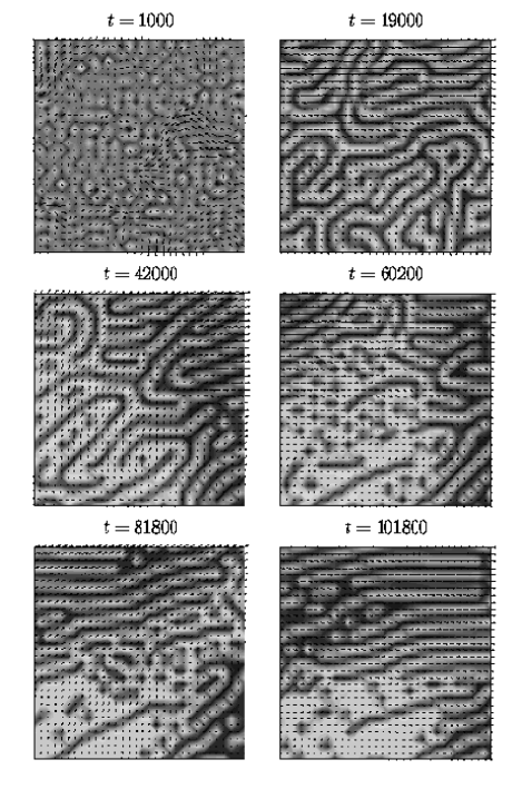
Figure 4: Configurations of the order parameter $\varphi$ on a central portion of size $128\times 128$ of the whole lattice for the case with $\gamma=5\times 10^{-5}$ and $\nu=4.1667$. Arrows represent fluid velocity vectors ${\bf u}$ and are plotted every four lattice sites.

Finally, in Fig. 4, the global patterns of the velocity field are shown for the same times of Fig. 1. We consider a central region of the system which includes a portion of the SIS phase and the interface with the lamellar region. At $t=1000$ there is no evidence of the imposed flow in this part of the system; local flows, as usually in phase segregation, originate from the defects. Effects of the imposed flow becomes evident at $t=19000$. Moving inside the SIS phase, the magnitude of the velocity vector becomes smaller with horizontal and vertical components comparable. Vortex structures, not present in the lamellar phase, can be also observed. In later pictures one observes that the SIS-lamellar interface structure evolves with time together with the local flow patterns. Velocity in the SIS phase always remains small and a jump in the velocity magnitude can be seen moving through the SIS-lamellar interface at all the late times considered.

IV Properties of SIS phase

The behavior described in the previous Section is found, at a given viscosity, for shear rates under a certain threshold. Velocity, stress and other properties, in cases when a SIS region is observed, have been checked to remain stable for long times and a linear velocity profile is never reached. Figure 5 shows the behavior of the chemical part of the stress for two values of shear rate smaller and larger than the threshold that, for the case $\nu=4.1667$, is $2.5\times 10^{-4}\lesssim\gamma_{c}\lesssim 5\times 10^{-4}$.

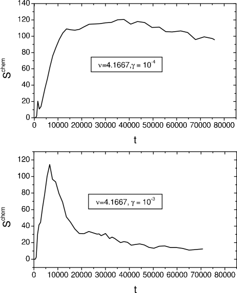
Figure 5: Plots of the integral chemical stress (Eq. (13)) as a function of time for two cases with different shear rates.

At $\gamma=10^{-4}$ the chemical stress remains almost stationary after the formation of the SIS region and the morphological evolution is similar to that shown in Figs. 1-2. On the other hand, at $\gamma=10^{-3}$, after a maximum, the shear stress decreases to small values while the horizontal velocity tends to a profile with constant slope. In this case the SIS region does not form in the middle of the system and ruptures do not occur at all in the lamellar network. Late-time configurations for the two cases are shown in Fig. 6. For $\gamma=10^{-3}$ one sees a well-ordered lamellar state with only few local defects.

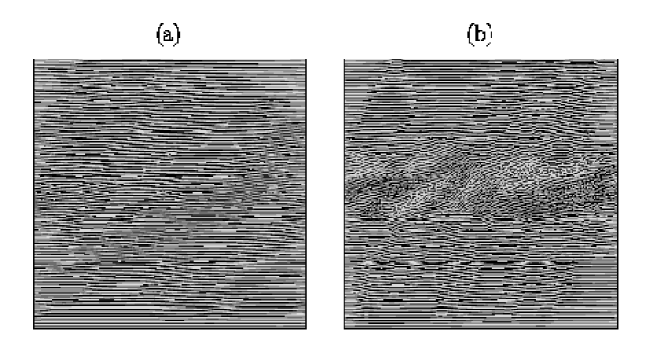
Figure 6: Late time configurations of the order parameter $\varphi$ on the whole $1024\times 1024$ lattice with $\nu=4.1667$ in the cases with $\gamma=10^{-3}$ at time $t=26400$ (a) and $\gamma=10^{-4}$ at time $t=73900$ (b).

For the case $\nu=4.1667$ we run various simulations with different values of $\gamma\leq\gamma_{c}$ also for comparing our results for the SIS phase with the usual scenario of shear banding Olmstedrev ; EYB ; olmsted ; hamley . In this scenario bands of phases with different structure and flow properties can coexist only at a critical value of the stress $S^{\star}$. In experiments with imposed shear rate this leads to a stress plateau on the flow curve (stress versus imposed shear rate) at $S^{\star}$. On the plateau, the shear rates of the different bands do not change by varying the imposed flow which only determines the relative spatial extension of the bands.

Figure 7: Plots of the $x$-averaged measured shear rate across the system for different imposed shear rates $\gamma$ with $\nu=4.1667$. Values are normalized to the imposed shear rate $\gamma$.

In Fig. 7 we show the shear rate profiles for different values of $\gamma<\gamma_{c}$ and for $\gamma=5\times 10^{-4}$ at times, for $\gamma<\gamma_{c}$, when the SIS phase is well formed. A central region with smaller shear rate can be clearly identified in all cases, except that for $\gamma=5\times 10^{-4}$. The width of this region, the one with SIS morphology, decreases when the imposed sear rate is increased, as usually in systems with shear banding. Close to the walls the shear rate is larger than the imposed value with an almost constant value in correspondence of the region with well aligned lamellae. However, differently from other systems with shear banding, the values of shear rates in the lamellar and in the SIS regions change with the imposed flow. The constraint that the integral of the horizontal velocity in the vertical direction gives the value imposed on the boundaries is always verified. An interface of finite width between the lamellar and the SIS region can be seen in all cases, confirming the relevance of the arguments discussed in Ref. olmsted .

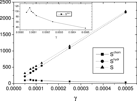
Figure 8: Plots of the different components of stress summed over the whole system at long times as functions of the imposed shear rate $\gamma$ for the case with $\nu=4.1667$. In the inset the chemical stress is plotted on a magnified scale for a better view.

The behavior of the hydrodynamical, chemical and total stress is shown in Fig. 8 as a function of the imposed shear rate. The total stress does not exhibit a flat regime in the interval where the SIS phase exists and changes in the behavior are not observed when $\gamma$ becomes greater than $\gamma_{c}$. As expected, the chemical stress decreases with the reduction of the width of the SIS region.

Finally, we examine the effects of viscosity showing results at fixed shear rate for times after the SIS formation. The main result is that at higher viscosities the width of the SIS region becomes narrower, as shown in Fig. 9. This behavior is confirmed from Fig. 10 where shear rate profiles are plotted.

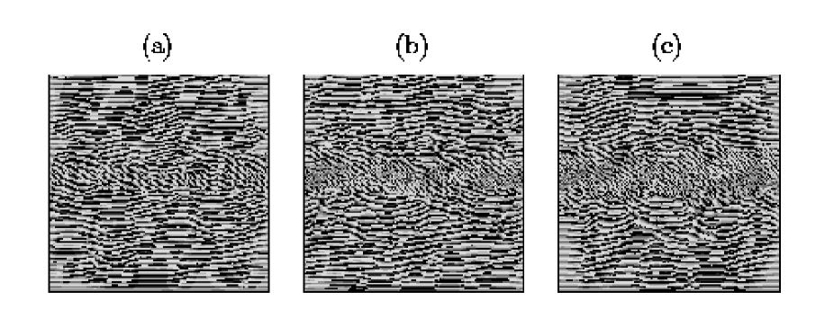
Figure 9: Configurations of the order parameter $\varphi$ on the whole $1024\times 1024$ lattice for the cases with $\gamma=10^{-4}$ and $\nu=15.883$ (a), $7.5$ (b), $4.1667$ (c).

Figure 10: Plots of the $x$-averaged measured shear rate across the system for different viscosities $\nu$ and $\gamma=10^{-4}$.

We have tried to interpret these results considering possible relations between cases with a SIS region and characteristic time scales of the imposed flow. The shear rate naturally introduces a typical time $\tau_{\gamma}=\gamma^{-1}$ when shear effects are expected to become relevant Onuki97 . On the other hand, the propagation of the horizontal velocity from the moving walls requires a relaxation time which, in simple fluids, is inversely proportional to the viscosity footnote2 . This time is also relevant for the effectiveness of the imposed flow in the middle of the system. We did not find a quantitative explanation of the phenomena before described in terms of these time scales, probably, also because the relaxation time of a simple fluid is not appropriate for the system we are studying. However, our results suggest the following general qualitative observation. If shear effects arrive early enough in the middle of the system, due to a large shear rate or to a high viscosity, the flow is able to penetrate in this region and lamellae align with it. Otherwise, at lower shear rates or lower viscosity, a SIS region can be found. We will return on this point in the discussion of the last Section.

V Domain Growth properties

In cases without imposed flows, the kinetics of formation of ordered phases after a quench is a process which is well-known for simple systems like binary mixtures, and still under investigations for lamellar systems. In binary mixtures dynamical scaling occurs with domains growing isotropically with power-law behavior B94 . In lamellar systems the formation of extended defects or grain boundaries between domains of differently oriented lamellae characterizes the late time evolution; other defects like dislocations and disclinations are also present Har00 ; BV02 ; Xuepl . Typical lengths can be defined and their evolution follow power-law or slower asymptotic growth depending on the steepness of the potential energy and on the depth of the quench. In cases with power-law behavior the length corresponding to the inverse of the structure factor at half height grows with an exponent ranging in the interval $0.2<z<0.33$ EVG92 ; BV01 ; CB98 ; Har00 ; YS02 ; QM02 ; Xuepl .

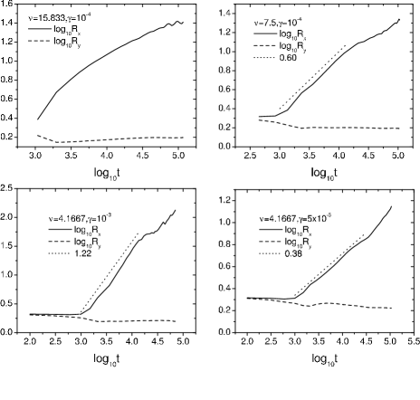
Figure 11: Plots of the domains sizes $R_{x}$ and $R_{y}$ as functions of time for different values of viscosities and imposed shear rates. See the single frames for parameters details and slopes of straight lines.

In our case with shear the presence of banded structures makes problematic the description of ordering in terms of a single length, as we have seen in the previous sections. However, it could still be interesting to consider the behavior of averaged lengths intended as macroscopic indicators of the degree of order in the system. We define

$$R_{\alpha}=\frac{\int d{\bf k}C({\bf k},t)}{\int d{\bf k}|k_{\alpha}|C({\bf k},t)}\;\;\;\;\;\;\;\alpha=x,y$$ (20)

and show in Fig. 11 the evolution of $R_{x},R_{y}$ for different viscosities and shear rates. In all cases $R_{y}$ relaxes to the equilibrium value, while $R_{x}$ grows with exponents $z_{x}$ varying with the viscosity and the shear rate as reported in the figure. In particular, keeping the viscosity $\nu$ fixed, we found that the value of $z_{x}$ increases by increasing the shear rate $\gamma$. In the case discussed in Section III with $\gamma=5\times 10^{-5}$ it results that $z_{x}=0.38$ for times $t\leq 40000$ corresponding to SIS formation; the later growth is characterized by the elimination of local defects in the lamellar region. Finite size effects may affect the behavior of $R_{x}$ at very late times. The case not shown in Fig. 11 with $\gamma=10^{-4}$ and the same viscosity $\nu=4.1667$ is similar. The time interval corresponding to the SIS formation ($t\leq 20000$) is characterized by a growth compatible with exponent $z_{x}=0.52$ while the growth rate changes later. By increasing further the shear rate ($\gamma=10^{-3}$), banded configurations do not form (see Figs. 5-6) and the whole system reaches a lamellar order with exponent $z_{x}\sim 1.2$. The behavior at $\gamma=10^{-4}$ and $\nu=7.5$ is qualitatively similar to those already discussed; the difference is in the value of the growth rate which is now $z_{x}=0.6$ during the SIS formation. We observe that this value is greater than in the case with the lower viscosity $\nu=4.1667$. Finally, for the highest value of viscosity shown in Fig. 11, a power law appears not appropriate for describing the behavior of $R_{x}$. We can conclude that the growth of lamellar order as measured by $R_{x}$ is faster for parameters corresponding to a smaller extension of the SIS region and a larger lamellar phase.

VI Discussion and Conclusions

In this paper we have shown results from two-dimensional simulation results for a fluid mixture quenched from a disordered configuration into a state with lamellar order. The fluid, described by Navier-Stokes and convection-diffusion equations, is subject during all the evolution to the action of a shear flow imposed by the walls of the system. The ordering process of a lamellar system, in absence of flow, would be characterized by the presence of local and extended defects that make slow, sometimes freezing, the evolution of the system. When shear is applied, defects tend to be eliminated and lamellae would be expected to align in a preferred direction forming well-ordered macroscopic domains.

Our results actually show that different evolutions with more complex morphologies are also possible under shear. For small enough shear rates and viscosities we found that the flow stabilizes itself with a horizontal velocity profile characterized by two different slopes. Close to the walls the shear rate is higher than the imposed one and well-ordered lamellae can be observed. In the central part of the system, that is reached later by the flow, the shear rate is smaller than the imposed one and the morphology of domains is characterized by the presence of small droplets and pieces of bent or rolled lamellae never aligned with the flow. We referred to this region as to a SIS phase.

Shear banding phenomena occur in many complex fluids. Similarly to what generally found, in our case the width of the SIS phase decreases by increasing the value of the imposed shear rate. In other important aspects, however, our results differ from the usual picture of shear banding. In the range of shear rates with coexisting lamellar and SIS regions, we do not observe a plateau of the total stress at varying shear intensity. Moreover, in this range, the values of local shear rates corresponding to the two phases depend on the imposed flow.

At the moment, we are not aware of experiments with the same scenario as that described in this paper. However, even if our model can be appropriately used for studying copolymer systems in the weak segregation limit Lei80 , the comparison with experiments is limited from the fact that our simulations are two-dimensional while in three-dimensional systems more complex geometries can occur fre ; hamley , with possible different rheological behaviors and flow patterns. Actually, the purpose of this work was more generic. We wanted to analyze general features of the formation of banded flows in systems with lamellar order considering the full dynamical problem for the velocity and the concentration fields.

Our results of Section III and IV show that when the applied flow is weak enough or propagates from the walls sufficiently slowly (at lower viscosities), it is not able to penetrate with the same shear rate in all the system. In this case the central region, with its intertwined tangled lamellae, opposes to the presence of the flow and tends to keep its morphology. The region tends to behave as an almost frozen network; the shear mainly acts stressing this network and causing ruptures with the production of droplets and small pieces of lamellae. Even if the shear rate in the SIS region is quite small but not zero, the behavior of our system resembles that of yield stress fluids where no flowing steady states exist for stresses under a certain threshold pabl . For example, in soft glass systems, coexistence between not flowing "pasty" states and sheared fluid regions has been observed v3b . In relation with this, it is interesting to observe that an equilibrium glass transition has been found also in systems with lamellar order SW00 . We think that in our case the competition between the intrinsic slow dynamics Xuepl and the acceleration induced by the external flow is responsible for the peculiar shear banding phenomena we have shown.

Finally, we observe that our numerical methods have been proven to be quite convenient for simulating fluids with complex order under driving forces. These methods can be implemented also with different geometries and in the more realistic three-dimensional case. We hope that our two-dimensional results can be useful for the comprehension of shear banding and stimulating for new experiments.

^(∗) Present address: Division of Physics and Astronomy, Yoshida-south Campus, Kyoto University, Sakyo-ku, Kyoto, 606-8501 Japan.

References

- (1) See, e.g., M. E. Cates and M. R. Evans, eds., Soft and Fragile Matter: Non Equilibrium Dynamics Metastability and Flow , IOP Publ., Bristol (2000).
- (2) R. G. Larson, The Structure and Rheology of Complex Fluids, Oxford University Press, New York (1998).
- (3) J. F. Berret, D. C. Roux, and G. Porte, J. Phys II 4, 1261 (1994).
- (4) E. Cappelaere, J. F. Berret, J. P. Decruppe, R. Cressely, and P. Lindner, Phys. Rev. E 56, 1869 (1997).
- (5) Y. T. Hu, P. Boltenhagen, and D. J. Pine, J. Rheol. 42, 1185 (1998).
- (6) P. Panizza, P. Archambault, and D. Roux, J. Phys. II 5, 303 (1995).
- (7) D. Roux, F. Nallet, and O. Diat, Europhys. Lett. 24, 53 (1993).
- (8) See, e.g., N. A. Spenley, M. E. Cates, and T. C. B. MacLeish, Phys. Rev. Lett. 71, 939 (1993); M. M. Britton and P.T. Callaghan, ibid. 78, 4930 (1997); J. B. Salmon, A. Colin, S. Manneville, and F. Molino, ibid. 90, 228303 (2003); J. B. Salmon, A. Colin, S. Manneville, Phys. Rev E 68 051503-4 (2003); D. Bonn, J. Meunier, O. Greffier, A. Alkahwaji, and H. Kellay, Phys. Rev. E 58, 2115 (1998); P. Panizza, L. Courbin, G. Cristobal, J. Rouch, and T. Narayanan, Physica A 322, 38 (2003).
- (9) J. D. Goddard, Annu. Rev. Fluid. Mech. 35, 113 (2003); J. Vermant, Curr. Opin. Colloid In. 6, 451 (2001); P. D. Olmsted, Curr. Opin. Colloid In. 4, 95 (1999).
- (10) P. Espanol, X. F. Yuan, and R. C. Ball, J. Non-Newtonian Fluid Mech. 65, 93 (1996); F. Greco and R. C. Ball, ibid. 69, 195 (1997).
- (11) P. D. Olmsted, Europhys. Lett. 48, 339 (1999).
- (12) A. Onuki, J. Phys.: Cond. Matter 9, 6119 (1997).
- (13) J. M. Yeomans, Ann. Rev. Comp. Physics VII, 61 (2000).
- (14) S.M. Fielding and P. D. Olmsted, Phys. Rev E 68, 036313 (2003).
- (15) S. A. Brazovskii, Sov. Phys. JETP 41, 85 (1975).
- (16) L. Leibler, Macromolecules 13, 1602 (1980); T. Ohta and K. Kawasaki, ibid. 19, 2621 (1986); G. H. Fredrickson and E. Helfand, J. Chem. Phys. 87, 697 (1987).
- (17) F. S. Bates and G. Fredrickson, Ann. Rev. Phys. Chem. 41, 525 (1990).
- (18) G. Gompper and M. Schick, Phase transitions and critical phenomena vol. 16, Academic, New York (1994).
- (19) C. Roland and R. C. Desai, Phys. Rev. B 42, 6658 (1990).
- (20) D. Kivelson, S. A. Kivelson, X. Zhao, Z. Nussinov, and G. Tarjus, Physica A 219, 27 (1995); M. Grousson, V. Krakoviack, G. Tarjus, and P. Viot, Phys. Rev. E 66, 026126 (2002)
- (21) S. C. Glotzer, E. A. Di Marzio, and M. Muthukumar, Phys. Rev. Lett. 74, 2034 (1995).
- (22) R. Benzi, S. Succi, and M. Vergassola, Phys. Rep. 222, 145 (1992); D. A. Wolf-Gladrow, Lattice gas cellular automata and lattice Boltzmann models, Springer-Verlag, New York (2000); S. Succi, The lattice Boltzmann equation, Oxford University Press, New York (2001).
- (23) G. Gonnella, E. Orlandini, and J. Yeomans, Phys. Rev. Lett. 78, 1695 (1997); Phys. Rev. E 58 , 480 (1998).
- (24) E. Orlandini, M. R. Swift, and J. M. Yeomans, Europhys. Lett. 32, 463 (1995); M. R. Swift, E. Orlandini, W. R. Osborn, and J. M. Yeomans, Phys. Rev. E 54, 5041 (1996).
- (25) A. Lamura and G. Gonnella, Physica A 294, 295 (2001).
- (26) X. Shan and H. Chen, Phys. Rev. E 47, 1815 (1993); ibid. 49, 2941 (1994); M. R. Swift, W. R. Osborn, and J. M. Yeomans, Phys. Rev. Lett. 75, 830 (1995); T. Ladd, J. Fluid Mech. 271, 285 (1994); ibid. 271, 311 (1994); A. Lamura, G. Gonnella, and J. M. Yeomans, Europhys. Lett. 45, 314 (1999).
- (27) C. Denniston, E. Orlandini, and J. M. Yeomans, Europhys. Lett. 52, 481 (2000); D. Marenduzzo, E. Orlandini, and J. M. Yeomans, Europhys. Lett. 64, 406 (2003).
- (28) Aiguo Xu, G. Gonnella, and A. Lamura, to appear in the Proceedings of the Discrete Simulations of Fluid Dynamics Conference, Boston, August 2004.
- (29) O. Filippova and D. Hänel, Int. J. Mod. Phys. C 9, 1439 (1998); J. Comput. Phys. 158, 139 (2000); P. Lallemand and L. S. Luo, Phys. Rev. E 68, 036706 (2003); R. Zhang and H. Chen, Phys. Rev. E 67, 066711 (2003).
- (30) Aiguo Xu, G. Gonnella, A. Lamura, G. Amati, and F. Massaioli, submitted to Europhys. Lett., cond-mat/0404205 (2004).
- (31) Y. Iwashita and H. Tanaka, to appear in Phys. Rev. Lett..
- (32) C.-Y. David Lu, P. D. Olmsted, and R. C. Ball, Phys. Rev. Lett. 84, 642 (2000).
- (33) R. Evans, Adv. Phys. 28, 143 (1979).
- (34) In terms of the chemical potentials and of the two components of a mixture one has .
- (35) P. Bhatnagar, E. P. Gross, and M. K. Krook, Phys. Rev. 94, 511 (1954).
- (36) Aiguo Xu, G. Gonnella, and A. Lamura, Phys. Rev. E 67, 056105 (2003); Aiguo Xu, G. Gonnella, and A. Lamura, Physica A 331, 10 (2004).
- (37) A. W. Lees and S. F. Edwards, J. Phys. C 5, 1921 (1972).
- (38) The relaxation time of a linear shear profile in a simple fluid is given by .
- (39) K. Matsuzaka, T. Koga, and T. Hashimoto, Phys. Rev. Lett, 80, 5441 (1998); F. Corberi, G. Gonnella, and A. Lamura, ibid. 81, 3852 (1998).
- (40) I. W. Hamley, J. Phys.: Cond. Matter 13, R643 (2001).
- (41) See, e.g., A. J. Bray, Adv. Phys. 43, 357 (1994).
- (42) D. Boyer and J. Viñals, Phys. Rev. E 65, 046119 (2002).
- (43) C. Harrison et al., Science 290, 1558 (2000); Phys. Rev. E 66, 011706 (2002).
- (44) Y. Yokojima and Y. Shiwa, Phys. Rev. E 65, 056308 (2002).
- (45) K. R. Elder, J. Viñals, and M. Grant, Phys. Rev. Lett. 68, 3024 (1992).
- (46) D. Boyer and J. Viñals, Phys. Rev. E 64, 050101(R) (2001).
- (47) J. J. Christensen and A. J. Bray, Phys. Rev. E 58, 5364 (1998).
- (48) H. Qian an G. F. Mazenko, Phys. Rev. E 67, 036102 (2003).
- (49) G. H. Fredrickson, J. Rheol. 38, 1045 (1994).
- (50) G. Picard, A. Adjari, L. Bocquet, and F. Lequeux, Phys. Rev. E 66, 051501 (2002).
- (51) F. Varnik, L. Bocquet, J. L. Barrat, and L. Berthier, Phys. Rev. Lett. 90, 095702 (2003).
- (52) J. Schmalian and P. G. Wolynes, Phys. Rev. Lett. 85, 836 (2000); M. Grousson, G. Tarjus, and P. Viot, ibid. 86, 3455 (2001); Cheng-Zhong Zhang and Zhen-Gang Wang, preprint cond-mat/0503536.