Critical currents in the BEC/BCS crossover regime

Abstract

Both the trapping geometry and the interatomic interaction strength of a dilute ultracold fermionic gas can be well controlled experimentally. When the interactions are tuned to strong attraction, Cooper pairing of neutral atoms takes place and a BCS superfluid is created. Alternatively, the presence of Feshbach resonances in the interatomic scattering allows populating a molecular (bound) state. These molecules are more tightly bound than the Cooper pairs and can form a Bose-Einstein condensate (BEC). In this contribution, we describe both the BCS and BEC regimes, and the crossover, from a functional integral point of view. In this description, the properties of the superfluid (such as vortices and Josephson tunneling) can be derived and followed as the system is tuned from BCS the BEC. In particular, we present results for the critical current of the superfluid through an optical lattice and link these results to recent experiments with atomic bosons in optical lattices.

I The ultracold dilute Fermi gas

When a dilute Bose gas is cooled below the degeneracy temperature, the bosonic atoms all condense in the same one-particle state and a Bose-Einstein condensate forms. This has been convincingly demonstrated with magnetically trapped, evaporatively cooled atomic gases for a multitude of atom species. Moreover, magnetic or optical traps can be equally well loaded with fermionic isotopes, such as ⁶Li or ⁴⁰K. These atoms do not undergo Bose-Einstein condensation, but fill up a Fermi sea, as has been demonstrated through the observation of the Pauli blocking effect DeMarcoSCI285 and through a measurement of the total energy of the Fermi gas DeMarcoPRL86 . Very soon after the observation of a degenerate Fermi sea of atoms, researchers embarked upon the quest to achieve Cooper pairing in the dilute Fermi gas. Indeed, for metals we know that the Fermi sea is unstable with respect to Cooper pair formation. So, if the (neutral) atoms in the dilute gas attract each other, a similar instability towards a paired state is to be expected.

The interatomic interactions in ultracold gases are remarkable for two reasons. Firstly, the collisions between the atoms can be satisfactorily characterized by a single number, the $s$-wave scattering length $a_{s}$. For low-energy collisions, the effective interaction potential between atoms becomes a contact potential, $V(\mathbf{r}-\mathbf{r}^{\prime})=g\delta(\mathbf{r}-\mathbf{r}^{\prime}),$ where $g=4\pi\hbar a_{s}/m$ with $m$ the mass of the atoms. The scattering length can be both positive (leading to interatomic repulsion) or negative (attraction).

Secondly, this scattering length can be tuned by an external magnetic field when a Feshbach resonance is present TiesingaPRA47 . This resonance occurs when the energy of a bound (molecular) state in a closed scattering channel becomes equal to the energy of the colliding atoms in the open scattering channel. The different channels correspond here to different hyperfine states of the trapped atoms, and the distance in energy between these states can be tuned with a magnetic field.

In what follows, we will consider a trapped mixture of ⁴⁰K atoms in the $\left|9/2,-7/2\right\rangle$ and $\left|9/2,-9/2\right\rangle$ hyperfine states. This potassium isotope is fermionic, and the trapped states display a Feshbach resonance at $B=202.1$ Gauss. When the scattering length is tuned to a negative value, the atoms attract and Cooper pairs can form leading to a BCS regime. The critical temperature for Cooper pairing can be raised by making the scattering length more strongly negative. When the scattering length is large and positive, the molecular state in the closed channel is populated, and molecules appear that can be Bose-Einstein condensed (the BEC regime). The adaptability of the scattering length allows bringing the gas from the BCS regime into the BEC regime or vice versa, and allows studying the interesting intermediate ‘crossover’ regime.

The first experimental realization of superfluidity of a Fermi gas in the molecular BEC regime came in 2003 ZwierleinPRL91 . A condensate of molecules was convincingly observed. The detection of superfluidity in the BCS regime however is much more subtle. In an initial experiment OHaraSCI298 , the superfluid behavior was derived from the hydrodynamic nature of the expansion of the cloud, as compared to a ballistic expansion expected for a non-superfluid weakly-interacting Fermi gas MenottiPRL89 . However, this did not constitute unambiguous proof, since the Fermi gas was in the strongly interacting regime. Subsequent experiments probed superfluidity by mapping the pair density onto a molecular condensate density RegalPRL92 or by spectroscopically measuring the gap BartensteinPRL92 . Yet although these experimental methods clearly demonstrate pairing, they do not unambiguously demonstrate superfluid behavior.

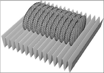
Figure 1: Two counterpropagating laser beams form a periodic potential for the atoms. Such optical lattices can be loaded with quantum gases, forming a stack of quasi-two dimensional clouds.

The very recent observation of a lattice of quantized vortices in resonant Fermi gases ZwierleinNAT435 constitutes the first clear demonstration of superfluidity in the BEC/BCS regime. Observation of these vortices well in the BCS regime may be difficult since the fermionic density penetrates in the core of the vortex in the BCS regime, leading to a loss of contrast in direct imaging BulgacJLTP138 ; TemperePRA71 ; ZwierleinNAT435 . Another possibility to demonstrate superconductivity is though the observation of the Josephson effect WoutersPRA70 in optical lattices. These optical lattices are periodic potentials formed by two counterpropagating laser beams, for example in the $z$-direction:

$$V_{opt}(z)=sE_{R}\sin^{2}(2\pi z/\lambda),$$ (1)

where $\lambda$ is the laser wave length, $E_{R}=h^{2}/(2m\lambda^{2})$ is the recoil energy, and $s$ is the laser intensity expressed in units of the recoil energy. Typically, $s=1-20$, $\lambda=795$ nm. The atoms collect in the valleys of the optical lattice and form a ”stack of pancakes”, illustrated in Fig. 1. Typically, there are on the order of a few 100 ‘pancakes’ with on the order of 1000 atoms each. When a superfluid is loaded in such an optical lattice, the system corresponds to an array of Josephson junctions. In such an array, the superfluid gas can propagate whereas the normal state gas is pinned. This has already been demonstrated for bosonic atoms CataliottiSCI293 , and has been predicted theoretically for fermionic atoms WoutersPRA70 ; OrsoPRL93 .

In this contribution, we derive and discuss the critical Josephson current for the flow of the superfluid component through an optical lattice. For this purpose, we base ourselves on the path-integral description as applied by Randeria and co-workers RanderiaPRB55 ; RanderiaPRL71 to the BEC/BCS crossover model of high-T_c superconductors. In section II, we give an overview of the application of path-integrals to the system of ultracold fermions, and in section III we present our results for the critical current.

II Path-integral treatment of the BEC/BCS crossover

The partition function for the atomic Fermi gas is given by the functional integral

$$\mathcal{Z}=\int\mathcal{D}\bar{\psi}_{\mathbf{x},\tau,\sigma}\mathcal{D}\psi_{\mathbf{x},\tau,\sigma}\text{ }\exp\left\{-\mathcal{S}/\hbar\right\}$$ (2)

with an action

$$\mathcal{S} ={\displaystyle\int\limits_{0}^{\hbar\beta}}d\tau\int d\mathbf{x}\text{ }{\textstyle\sum_{\sigma}}\bar{\psi}_{\mathbf{x},\tau,\sigma}\left(\hbar\frac{\partial}{\partial\tau}-\frac{\hbar^{2}}{2m}\nabla_{\mathbf{x}}^{2}-\mu\right)\psi_{\mathbf{x},\tau,\sigma}$$

$$+{\displaystyle\int\limits_{0}^{\hbar\beta}}d\tau\int d\mathbf{x}\text{ }g\bar{\psi}_{\mathbf{x},\tau,\uparrow}\bar{\psi}_{\mathbf{x},\tau,\downarrow}\psi_{\mathbf{x},\tau,\downarrow}\psi_{\mathbf{x},\tau,\uparrow}.$$ (3)

The fermionic fields $\psi_{\mathbf{x},\tau},\bar{\psi}_{\mathbf{x},\tau}$ are Grassman variables. The interaction potential, as discussed in the previous section, is a contact potential with experimentally adjustable strength $g$. The two hyperfine states are denoted by $\sigma=\uparrow,\downarrow$. The functional integral over the Grassman variables can be performed analytically only for an action that is quadratic in $\psi_{\mathbf{x},\tau},\bar{\psi}_{\mathbf{x},\tau}$. In order to get rid of the quartic term in (3) we perform a Hubbard-Stratonovic (HS) transformation, introducing auxiliary bosonic fields $\bar{\Delta}_{\mathbf{x},\tau}$ and $\Delta_{\mathbf{x},\tau}$ :

$$\mathcal{Z}\propto\int\mathcal{D}\bar{\psi}_{\mathbf{x},\tau,\sigma}\mathcal{D}\psi_{\mathbf{x},\tau,\sigma}\int\mathcal{D}\bar{\Delta}_{\mathbf{x},\tau}\mathcal{D}\Delta_{\mathbf{x},\tau}\text{ }\exp\left\{-\mathcal{S}/\hbar\right\}$$ (4)

with

$$\mathcal{S} ={\displaystyle\int\limits_{0}^{\hbar\beta}}d\tau\int d\mathbf{x}\text{ }{\textstyle\sum_{\sigma}}\bar{\psi}_{\mathbf{x},\tau,\sigma}\left(\hbar\frac{\partial}{\partial\tau}-\frac{\hbar^{2}}{2m}\nabla_{\mathbf{x}}^{2}-\mu\right)\psi_{\mathbf{x},\tau,\sigma}$$

$$-{\displaystyle\int\limits_{0}^{\hbar\beta}}d\tau\int d\mathbf{x}\text{ }\left(\bar{\Delta}_{\mathbf{x},\tau}\psi_{\mathbf{x},\tau,\downarrow}\psi_{\mathbf{x},\tau,\uparrow}+\Delta_{\mathbf{x},\tau}\bar{\psi}_{\mathbf{x},\tau,\uparrow}\bar{\psi}_{\mathbf{x},\tau,\downarrow}+\frac{\bar{\Delta}_{\mathbf{x},\tau}\Delta_{\mathbf{x},\tau}}{g}\right).$$ (5)

Indeed, performing the functional integral over the HS fields $\bar{\Delta}_{\mathbf{x},\tau}$,$\Delta_{\mathbf{x},\tau}$ in (5) brings us back to (3). Our goal is an investigation of the superfluid properties of the ultracold Fermi system. For a straightforward hydrodynamic interpretation of the Hubbard-Stratonovic fields, it is advantageous to work with $\left|\Delta_{\mathbf{x},\tau}\right|$ and $\theta_{\mathbf{x},\tau}$. These are related to the original HS field by $\Delta_{\mathbf{x},\tau}=\left|\Delta_{\mathbf{x},\tau}\right|\exp(i\theta_{\mathbf{x},\tau})$. We have restricted the functional integral to $\bar{\Delta}_{\mathbf{x},\tau}=(\Delta_{\mathbf{x},\tau})^{\ast}$ without neglecting any field configurations of importance to the final result. The hydrodynamic interpretation of $\left|\Delta_{\mathbf{x},\tau}\right|^{2}$ is the density of fermion pairs, whereas $\hbar\mathbf{\nabla}_{\mathbf{x}}\theta_{\mathbf{x},\tau}/m=\mathbf{v}_{\mathbf{x},\tau}$ can be interpreted as the superfluid velocity field. Performing this change of variables in the functional integral yields

$$\mathcal{Z}\propto\int\mathcal{D}\bar{\psi}_{\mathbf{x},\tau,\sigma}\mathcal{D}\psi_{\mathbf{x},\tau,\sigma}\int\mathcal{D}\left|\Delta_{\mathbf{x},\tau}\right|\mathcal{D}\theta_{\mathbf{x},\tau}\text{ }\exp\left\{-\mathcal{S}/\hbar\right\},$$ (6)

with

$$\mathcal{S} ={\displaystyle\int\limits_{0}^{\hbar\beta}}d\tau\int d\mathbf{x}\text{ }\bar{\psi}_{\mathbf{x},\tau,\sigma}\left(\hbar\frac{\partial}{\partial\tau}-\frac{\hbar^{2}}{2m}\nabla_{\mathbf{x}}^{2}-\frac{1}{2}\mathbf{v_{\mathbf{x},\tau}}\cdot i\hbar\mathbf{\nabla}_{\mathbf{x}}-\mu\right.$$

$$\qquad\qquad\qquad+\left.\frac{i\hbar}{2}\frac{\partial\theta_{\mathbf{x},\tau}}{\partial\tau}-\frac{1}{4}\left(i\hbar\mathbf{\nabla}_{\mathbf{x}}\cdot\mathbf{v}_{\mathbf{x},\tau}\right)+\frac{1}{8}m\mathbf{v}_{\mathbf{x},\tau}^{2}\right)\psi_{\mathbf{x},\tau,\sigma}$$

$$-{\displaystyle\int\limits_{0}^{\hbar\beta}}d\tau\int d\mathbf{x}\text{ }\left(\left|\Delta_{\mathbf{x},\tau}\right|\psi_{\mathbf{x},\tau,\downarrow}\psi_{\mathbf{x},\tau,\uparrow}+\left|\Delta_{\mathbf{x},\tau}\right|\bar{\psi}_{\mathbf{x},\tau,\uparrow}\bar{\psi}_{\mathbf{x},\tau,\downarrow}+\frac{\left|\Delta_{\mathbf{x},\tau}\right|^{2}}{g}\right).$$ (7)

De Palo et al. DePaloPRB60 suggest at this point to introduce additional collective quantum variables to extract the fermionic density. However, care must be taken, since when additional collective quantum fields are present the problem of double-counting poses itself KleinertFP26 , and variational perturbation theory has to be applied to avoid double-counting KleinertAP266 . However, in the present case it is not necessary to explicitly introduce the additional collective variables to obtain information about the atomic density profile PelsterPC . In (6) the integration over the fermionic variables can be taken, leading to

$$\mathcal{Z}\propto\int\mathcal{D}\left|\Delta_{\mathbf{x},\tau}\right|\mathcal{D}\theta_{\mathbf{x},\tau}\text{ }\exp\left\{-\mathcal{S}_{\text{eff}}/\hbar\right\}$$ (8)

with an effective action

$$\mathcal{S}_{\text{eff}}=-\hbar\operatorname*{tr}\left[\ln\left(\frac{-\mathbb{G}^{-1}}{\hbar}\right)\right]-{\displaystyle\int\limits_{0}^{\hbar\beta}}d\tau\int d\mathbf{x}\text{ }\frac{\left|\Delta_{\mathbf{x},\tau}\right|^{2}}{g}.$$ (9)

where the inverse propagator can be written as the sum of an inverse ‘free fermion propagator’ and a term arising from the superfluidity:

$$-\mathbb{G}^{-1}=-\mathbb{G}_{0}^{-1}+\mathbb{S}$$ (10)

The inverse free fermion propagator is

$$-\mathbb{G}_{0}^{-1}=\sigma_{0}\left(\hbar\frac{\partial}{\partial\tau}\right)+\sigma_{3}\left(-\frac{\hbar^{2}}{2m}\mathbf{\nabla}_{\mathbf{x}}^{2}-\mu\right).$$ (11)

and the superfluid part of the propagator can be written as

$$\mathbb{S} =\sigma_{0}\left(-\frac{1}{2}\mathbf{v_{\mathbf{x},\tau}}\cdot i\hbar\mathbf{\nabla}_{\mathbf{x}}\right)-\sigma_{1}(\hbar\left|\Delta_{\mathbf{x},\tau}\right|)$$

$$+\sigma_{3}\left(\frac{i\hbar}{2}\frac{\partial\theta_{\mathbf{x},\tau}}{\partial\tau}-\frac{1}{4}i\hbar\mathbf{\nabla}_{\mathbf{x}}\cdot\mathbf{v}_{\mathbf{x},\tau}+\frac{1}{8}m\mathbf{v}_{\mathbf{x},\tau}^{2}\right).$$ (12)

In these expressions, $\sigma_{0}...\sigma_{3}$ are the Pauli matrices. Note that if we have an external potential $V_{ext}(\mathbf{x)}$ present, for example the optical potential or the magnetic trap, this appears in $-\mathbb{G}_{0}^{-1}$ as an extra term $+\sigma_{3}V_{ext}(\mathbf{x)}$. The effective action (9) depends on the fields $\left|\Delta_{\mathbf{x},\tau}\right|,\theta_{\mathbf{x},\tau}$ and $\rho_{\mathbf{x},\tau},\zeta_{\mathbf{x},\tau}$. For the former, a saddle point approximation is usually made. For example, a good saddle point form when no vortex is present is RanderiaPRL71 ; RanderiaPRB55 :

$$\left\{\begin{array}[c]{c}\left|\Delta_{\mathbf{x},\tau}\right|=\Delta\\ \theta_{\mathbf{x},\tau}=\text{constant.}\end{array}\right.$$ (SP1)

The value of the constant for the phase is irrelevant, and the value of $\Delta$ can be extracted by extremizing the effective action $\delta\mathcal{S}_{\text{eff}}/\delta\Delta=0$. This yields the well-known gap equation in the case of neutral atoms interacting through a contact potential. Alternatively, we proposed in Ref. TemperePRA71 to use a different saddle point approximation to investigate the case of a fermionic superfluid containing a vortex parallel to the $z$-axis:

$$\left\{\begin{array}[c]{c}\left|\Delta_{\mathbf{x},\tau}\right|=\Delta_{r}\\ \theta_{\mathbf{x},\tau}=\phi\text{.}\end{array}\right.$$ (SP2)

Here, $\phi$ is the angle around the $z$-axis, and $r$ is the distance to the $z$-axis. Again, a gap equation can be derived for $\Delta_{r}$ by extremizing the action - this gap equation yields a gap that depends on the distance to the vortex line (the $z$-axis). Fixing the total number of fermions yields a number equation in which the local density of fermions can be identified straightforwardly.

Consider first the simplest saddle point approximation, (SP1). The saddle point result for the action in this case is

$$\mathcal{S}_{\text{sp1}}=\frac{\left|\Delta\right|^{2}}{g}\left.-2\int\dfrac{d\mathbf{k}}{(2\pi)^{3}}\ln\left[2\cosh\left(\dfrac{\beta}{2}\sqrt{\left(\dfrac{k^{2}}{2m}-\mu\right)^{2}+\left|\Delta\right|^{2}}\right)\right]\right\}.$$ (13)

Two unknowns are the chemical potential $\mu$ and the value of constant $\Delta$, the gap. The chemical potential is obtained by fixing the particle density. In the BCS limit, $\mu\rightarrow E_{F}$ whereas in the BEC limit, the chemical potential goes to the binding energy of the molecule, $\mu\rightarrow\hbar^{2}/(ma_{s}^{2})$. In the intermediate regime, there is a smooth crossover between the two limiting values. The gap $\Delta$ is found by extremizing the saddle point action, $\delta\mathcal{S}_{\text{sp1}}/\delta\Delta=0$. The result is shown for different temperatures in figure 2. At temperature zero, the gap depends exponentially on the scattering length as we expect from the BCS theory. As the temperature is raised, the gap decreases, reaching zero at a certain temperature. In the BCS limit, the superfluidity is destroyed by breaking up Cooper pairs, so the critical temperature corresponds to the temperature where $\Delta=0$. However, in the BEC limit, superfluidity is destroyed through phase fluctuations, and one cannot extract the critical temperature from the results shown in figure 2. It becomes necessary to include fluctuations around the saddle point value (SP1) and expand the effective action up to second order in these fluctuations around the saddle point value. This second-order expansion yields an action that is quadratic in the fluctuation variables and that can be integrated analytically. For fluctuations around the saddle point (SP1) this was done by Randeria and co-workers, who obtained a corrected value of the critical temperature that in the BEC limit becomes independent of $1/(k_{F}a_{s})$. More recently, the effects of fluctuations in the superfluid regime, in the context of a diagrammatic expansion of the thermodynamic potential in refs. PeraliPRL92 ; HuCM .

Figure 2: The saddle point value $\Delta~{}$is shown as a function of the interaction strength parameter $1/(k_{F}a_{s})$ for different values of the temperature. In the BCS regime this corresponds to the BCS gap and it vanishes at the critical temperature. The inset shows the temperature at which $\Delta=0$. In the BEC regime, fluctuations around the saddle point need to be taken into account to obtain the correct critical temperature RanderiaPRL71 ; PeraliPRL92 ; HuCM .

III Determination of the critical current

III.1 Effective action in the optical potential

The path-integral method outlined in the previous section has been applied before to describe vortices in a superfluid Fermi gas TemperePRA71 and to describe the propagation of a superfluid Fermi gas in an optical potential WoutersPRA70 . When an optical lattice (1) is present along the $z$-direction, we can decouple the (free) motion in the $x,y$-plane from the (tunneling) motion in the $z$-direction. To make this decoupling clear in the notations, we write the partition function of the system as

$$\mathcal{Z}=\int\mathcal{D}\bar{\psi}_{j,\sigma}(r)\mathcal{D}\psi_{j,\sigma}(r)\text{ }\exp\left\{-\mathcal{S}/\hbar\right\},$$ (14)

with $r=\{x,y,\tau\}$ and

$$\mathcal{S}=\sum_{j}\mathcal{S}_{j}+\sum_{j}\mathcal{S}_{j\rightarrow j+1}^{tunnel}.$$ (15)

The action functional for the gas in layer $j$ separately is given by

$$\mathcal{S}_{j} ={\displaystyle\int\limits_{0}^{\hbar\beta}}d\tau\int d\mathbf{x}\text{ }{\textstyle\sum_{\sigma}}\bar{\psi}_{j,\sigma}(r)\left(\hbar\frac{\partial}{\partial\tau}-\frac{\hbar^{2}}{2m}\nabla_{\mathbf{x}}^{2}-V_{ext}(j)-\mu\right)\psi_{j,\sigma}(r)$$

$$+{\displaystyle\int\limits_{0}^{\hbar\beta}}d\tau\int d\mathbf{x}\text{ }g\bar{\psi}_{j,\uparrow}(r)\bar{\psi}_{j,\downarrow}(r)\psi_{j,\downarrow}(r)\psi_{j,\uparrow}(r).$$ (16)

This is the two-dimensional version of the action functional (3), supplemented with a layer index. Moreover, there is an external potential $V_{ext}(j)$ acting on each layer. This can a parabolic potential in addition to the optical potential itself. The tunneling of atoms from one layer to another is described by

$$\mathcal{S}_{j\rightarrow j+1}^{tunnel}={\displaystyle\int\limits_{0}^{\hbar\beta}}d\tau\int d\mathbf{x}\text{ }t_{1}\sum_{\sigma}\left[\bar{\psi}_{j,\sigma}(r)\psi_{j+1,\sigma}(r)+\bar{\psi}_{j+1,\sigma}(r)\psi_{j,\sigma}(r)\right],$$ (17)

where the tunneling energy $t_{1}$ to bring an atom from one well of the optical potential to the next was derived in Ref. MartikainenPRA68 :

$$t_{1}=sE_{R}\left[\frac{\pi^{2}}{4}-1\right]e^{-\sqrt{s}(\pi/2)^{2}}.$$ (18)

For this particular decomposition of the action functional in intralayer contributions and tunneling contributions, we can perform the same analysis as described in the previous section. A Hubbard-Stratonovich transformation gets rid of the four-operator term and introduces the HS fields $\left|\Delta_{j}\right|,\theta_{j}$, after which the integration over fermionic variables is performed. The final result for the effective action can again be written as the sum of contributions independent of $t_{1}$ and tunneling contributions:

$$\mathcal{S}_{\text{eff}}=\sum_{j}\mathcal{S}_{\text{eff,}j}+\sum_{j}\mathcal{S}_{\text{eff, }j\rightarrow j+1}^{tunnel}.$$ (19)

The effective action for layer $j$ is

$$\mathcal{S}_{\text{eff,}j}=-\hbar\operatorname*{tr}\left[\ln\left(\frac{-\mathbb{G}_{\text{sp}}^{-1}}{\hbar}\right)\right]-{\displaystyle\int\limits_{0}^{\hbar\beta}}d\tau\int d\mathbf{x}\text{ }\frac{\left|\Delta_{j}\right|^{2}}{g}$$ (20)

with

$$-\mathbb{G}_{\text{sp}}^{-1}=\sigma_{0}\left(\hbar\frac{\partial}{\partial\tau}\right)+\sigma_{3}\left(-\frac{\hbar^{2}}{2m}\mathbf{\nabla}_{\mathbf{x}}^{2}-V_{ext}\left(j\right)-\mu\right)-\sigma_{1}(\hbar\left|\Delta_{j}\right|).$$ (21)

The tunneling contributions in the effective action can be treated perturbatively. In that framework, the saddle-point values $\left|\Delta_{j}\right|$ can be extracted from the gap equation of each layer separately, and the chemical potential $\mu$ is obtained from the number equation. In each layer $j$, there is an ‘effective’ chemical potential $V_{ext}\left(j\right)+\mu$ fixing the local density $\rho_{j}$ in layer $j$. Based on these results for the layers, the lowest-order perturbative expansion of the action with respect to the tunneling part ($t_{1}$) yields

$$\mathcal{S}_{\text{eff, }j\rightarrow j+1}^{tunnel}=-{\displaystyle\int\limits_{0}^{\hbar\beta}}d\tau\int d\mathbf{x}\text{ }T_{j\rightarrow j+1}\cos[\theta_{j+1}-\theta_{j}]$$ (22)

with,

$$T_{j\rightarrow j+1}=\frac{t_{1}^{2}\rho_{j}}{2\pi\hbar^{2}\rho_{j}/m+E_{b}},$$ (23)

where $E_{b}$ is the binding energy of the molecule. This molecular binding energy appears through the gap equations and can be derived from scattering theory in reduced dimensionality. It is given by PetrovPRA64 :

$$E_{b}^{\text{2D}}=0.583\sqrt{s}E_{R}\exp\left(\frac{1}{\sqrt{2\pi}}\frac{\lambda}{s^{-1/4}a_{s}}\right).$$ (24)

It is important to note that the binding energy depends on the intensity and wavelength of the lasers generating the optical potential. More intense laser beams or smaller wavelengths confine the gas more strongly in the optical lattice and alter the binding energy of the resonant molecules. A more detailed determination of the molecular binding energy in an optical lattice, taking into account molecules formed from atoms in neighboring lattice sites, is given in Ref. WoutersCM .

III.2 Coupled density-phase equations

The equations of motion for the remaining variables (density $\rho_{j}$ and phase $\theta_{j}$ in layer $j$) can be derived from the effective action (19)-(22) through the extremum conditions $\delta S_{\text{eff}}/\delta\theta_{j}=0$ and the number equation. This leads to the equations reported by the present authors and M. Wouters in Ref. WoutersPRA70 :

$$\hbar\partial_{t}\frac{\rho_{j}\left(x\right)}{2} =-\frac{\mathbf{\nabla}\theta_{j}\cdot\mathbf{\nabla}\rho_{j}}{4m}$$

$$+T_{j,j-1}\sin\left(\theta_{j}-\theta_{j-1}\right)$$

$$-T_{j+1,j}\sin\left(\theta_{j+1}-\theta_{j}\right),$$ (25)

and

$$-\hbar\partial_{t}\frac{\theta_{j}}{2} =\frac{\left[\nabla\theta_{j}\right]^{2}}{8m}+V_{ext}\left(j\right)-\mu$$

$$-\frac{\partial T_{j+1,j}}{\partial\rho_{j}}\cos\left(\theta_{j+1}-\theta_{j}\right)$$

$$-\frac{\partial T_{j,j-1}}{\partial\rho_{j}}\cos\left(\theta_{j}-\theta_{j-1}\right).$$ (26)

In these equations, we have introduced the possibility of applying an external potential $V_{ext}(j)$ varying over the layers. Here, we investigate the case with a constant phase difference $\theta_{j+1}-\theta_{j}=\Delta\theta$ and a smoothly varying density $\rho_{j+1}\approx\rho_{j}$. This situation corresponds to a uniform flow of superfluid through the lattice. Then equations (25),(26) simplify to

$$\hbar\partial_{t}\frac{\rho_{j}}{2} =\frac{t_{1}^{2}}{2\pi\hbar^{2}\rho_{j}/m+E_{b}}\rho_{j}\sin(\Delta\theta)$$ (27)

$$-\hbar\partial_{t}\frac{\Delta\theta}{2} =\nabla_{j}\left[V_{ext}\left(j\right)\right]-\frac{t_{1}^{2}E_{b}}{[2\pi\hbar^{2}\rho_{j}/m+E_{b}]^{2}}\cos(\Delta\theta)$$ (28)

In the BEC case, $E_{b}\gg\hbar^{2}\rho_{j}/m$ and we retrieve the equations describing a conventional Josephson junction array. However, on the BCS side, the tunneling coefficients start to depend on $\rho_{j}$, as $E_{b}$ and $\hbar^{2}\rho_{j}/m$ become comparable.

III.3 Critical Josephson current and critical velocity

Equation (27) states that the current density $J$ is proportional to $\sin(\Delta\theta)$. This is similar to the first Josephson equation,

$$J=J_{c}\sin(\Delta\theta).$$

The second equation, (28), fixes the time derivative of the phase difference to the differences in potential energy of the gas in the different wells. Near $\Delta\theta=0,\pi/2$ equation (28) yields the second Josephson equation $-\hbar d(\Delta\theta)/dt=\Delta U$ where $\Delta U$ is the difference in energy between consecutive wells for the molecules. From the first Josephson equation we can extract a critical current by setting $\Delta\theta=\pi/2,$ as has been done for bosonic atoms in the optical lattice in Ref. SmerziPRL89 . This yields a critical current density for Josephson tunneling from layer to layer:

$$J_{c}=\frac{2}{\hbar}\frac{t_{1}^{2}}{2\pi\hbar^{2}\rho_{j}/m+E_{b}}\rho_{j},$$ (29)

The layers are separated by a distance $\lambda/2$. From $J_{c}$ we can then extract the critical velocity for the fermionic atoms through the optical lattice,

$$v_{c}=\frac{t_{1}^{2}}{2\pi\hbar^{2}\rho_{j}/m+E_{b}}\frac{\lambda}{\hbar}.$$ (30)

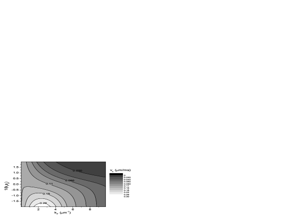
Figure 3: The critical Josephson velocity through the optical lattice, in microns/ms, is shown as a function of the interaction strength parameter $1/(k_{F}a_{s})$ and the Fermi wavevector of the 2D fermi gas in the valleys. In the upper half ($a_{s}>0$) of the figure the BEC regime develops, and in the lower half ($a_{s}<0$) the BCS regime appears. The optical lattice parameters are $\lambda=795$ nm and $s=3$. The atom parameters correspond to ⁴⁰K atoms in the $\left|9/2,-7/2\right\rangle$ and $\left|9/2,-9/2\right\rangle$ hyperfine states, having a Feshbach resonance at $B=202.1$ Gauss.

The critical velocity of the fermionic superfluid depends on the scattering length $a_{s},$ via the binding energy of the Feshbach resonant molecule, $E_{b}$. The critical velocity also depends on the density (or, equivalently, the Fermi wave vector). In Figure 3 we show the results for the critical velocity (expressed in microns per millisecond), as a function of $k_{F}$ and of the interaction parameter $1/(k_{F}a_{s})$. In the region $1/(k_{F}a_{s})>0$ we are in the molecular BEC regime, and $E_{b}\gg\hbar^{2}\rho_{j}/m$. The critical velocity in the BEC regime is roughly proportional to $t_{1}^{2}/E_{b}$. In the region $1/(k_{F}a_{s})<0,$ the BCS regime of Cooper pairs arises, and the result for the critical velocity becomes nontrivial. For each fixed value of $1/(k_{F}a_{s})<0,$ there appears a maximum as a function of $k_{F}$. This maximum occurs when $E_{b}\approx\hbar^{2}\rho_{j}/m$, minimizing the denominator in (30).

Although superfluid gases of bosonic atoms have already been studied in optical lattices CataliottiSCI293 ; CataliottiNJP5 , superfluid Fermi gases have to this moment not been loaded in optical lattices. Also no molecular condensates have been placed in optical lattices. For atomic condensates, a critical velocity could be determined experimentally CataliottiNJP5 , and was found to vary between $0.2$ and $1.2$ $\mu$m/ms for ⁸⁷Rb atoms. This is comparable to the velocities that we predict for (fermionic) ⁴⁰K in the same $\lambda=795$ optical potential. Thus, the superfluid regime of paired fermionic atoms in an optical lattice should be accessible experimentally.

IV Conclusions

The path-integral description of ultracold fermionic atoms interacting through a tunable contact potential allows to describe vortex configurations and other non-ground state configurations through a judicious choice of saddle point. We apply this formalism to the case of a fermionic gas in an optical potential. When the fermionic gas is in the superfluid regime, the layers of gas in the optical potential form a Josephson junction array. Equations of motion for the density and phase in each layer are obtained and applied to the case where the phase difference between consecutive layers is constant. This permits the derivation of a critical velocity of the superfluid flow through the optical potential. Although these results are strictly speaking derived for $T=0,$ in the experiments the temperature can typically be brought down well below the degeneracy temperature so that we believe our results will be relevant to the experiments with optical lattices.

- (1) B. DeMarco and D.S. Jin, Science 285, 1703 (1999).
- (2) B. DeMarco, S.B. Papp, and D.S. Jin, Phys. Rev. Lett. 86, 5409 (2001).
- (3) E. Tiesinga, B. J.Verhaar, and H.T.C. Stoof, Phys. Rev. A 47, 4114 (1993).
- (4) M. W. Zwierlein, C. A. Stan, C. H. Schunck, S. M. F. Raupach, S. Gupta, Z. Hadzibabic, and W. Ketterle, Phys. Rev. Lett. 91, 250401 (2003).
- (5) K. M. O’Hara, S. L. Hemmer, M. E. Gehm, S. R. Granade, and J. E. Thomas, Science 298, 2179 (2002).
- (6) C. Menotti, P. Pedri, and S. Stringari, Phys. Rev. Lett. 89, 250402 (2002).
- (7) C. A. Regal, M. Greiner, D.S. Jin, Phys. Rev. Lett. 92, 040403 (2004).
- (8) M. Bartenstein, A. Altmeyer, S. Riedl, S. Jochim, C. Chin, J. H. Denschlag, and R. Grimm, Phys. Rev. Lett. 92, 120401 (2004).
- (9) M.W. Zwierlein, J. R. Abo-Shaeer, A. Schirotzek, C.H. Schunck, and W. Ketterle, Nature 435, 1047 (23/6/2005).
- (10) A. Bulgac, Y. Yu, J. Low Temp. Phys. 138, 741 (2005).
- (11) J. Tempere, M. Wouters, and J.T. Devreese, Phys. Rev. A 71, 033631 (2005).
- (12) M. Wouters, J. Tempere, and J.T. Devreese, Phys. Rev. A 70, 013616 (2004).
- (13) F. S. Cataliotti, S. Burger, C. Fort, P. Maddaloni, F. Minardi, A. Trombettoni, A. Smerzi, and M. Inguscio, Science 293, 843 (2001).
- (14) G. Orso, L. P. Pitaevskii, and S. Stringari, Phys. Rev. Lett. 93, 020404 (2004).
- (15) C. A. R. Sá de Melo, M. Randeria, and J. R. Engelbrecht, Phys. Rev. Lett. 71, 3202 (1993).
- (16) J. R. Engelbrecht, M. Randeria, and C. A. R. Sá de Melo, Phys. Rev. B 55, 15153 (1997).
- (17) S. De Palo, C. Castellani, C. Di Castro and B. K. Chakraverty, Phys. Rev. B 60, 564 (1999).
- (18) H. Kleinert, Fortschr. Physik 26, 565 (1978).
- (19) H. Kleinert, Annals of Physics 266, 135 (1998).
- (20) A. Pelster, private communication.
- (21) A. Perali, P. Pieri, L. Pisani, and G. C. Strinati, Phys. Rev. Lett. 92, 220404 (2004).
- (22) H. Hu, X.-J. Liu, and P. D. Drummond, cond-mat/0506046.
- (23) J.-P. Martikainen, H. T. C. Stoof, Phys. Rev. A 68, 013610 (2003).
- (24) D.S. Petrov and G.V. Shlyapnikov, Phys. Rev. A 64, 012706 (2001).
- (25) G. Orso, L.P. Pitaevskii, S. Stringari, M. Wouters, cond-mat/0503096.
- (26) A. Smerzi, A. Trombettoni, P.G. Kevrekidis, and A. R. Bishop, Phys. Rev. Lett. 89, 170402 (2002).
- (27) F. S. Cataliotti, L. Fallani, F. Ferlaino, C. Fort, P. Maddaloni, M. Inguscio, New Journal of Physics 5, 71 (2003).