Precipitation in Al-Zr-Sc alloys:
a comparison between kinetic Monte Carlo, cluster dynamics
and classical nucleation theory

Emmanuel Clouet,¹ Maylise Nastar,¹ Alain Barbu,¹ Christophe Sigli,² Georges Martin³

Abstract

Zr and Sc precipitate in aluminum alloys to form the Al₃Zr_xSc_1-x compound which, for low supersaturations of the solid solution, exhibits the L1₂ structure. The aim of the present study is to model at an atomic scale the kinetics of precipitation and to build mesoscopic models so as to extend the range of supersaturations and annealing times that can be simulated up to values of practical interest. In this purpose, we use some ab initio calculations and experimental data to fit an Ising type model describing thermodynamics of the Al-Zr-Sc system. Kinetics of precipitation are studied with a kinetic Monte Carlo algorithm based on an atom-vacancy exchange mechanism. Cluster dynamics is then used to model at a mesoscopic scale all the different stages of homogeneous precipitation in the two binary Al-Zr and Al-Sc alloys. This technique correctly manages to reproduce both the kinetics of precipitation simulated with kinetic Monte Carlo as well as experimental observations. Focusing on the nucleation stage, it is shown that classical theory well applies as long as the short range order tendency of the system is considered. This allows us to propose an extension of classical nucleation theory for the ternary Al-Zr-Sc alloy.

Introduction

Transition elements like Mn, Cr, Zr or Sc are usually added to aluminum alloys so as to form small ordered precipitates which increase the tensile strength and inhibit recrystallization. As these properties directly depend on the density and the size of the particles, an accurate control of the precipitation process is necessary so as to optimize the material. In particular, one can use a combined addition of solute elements so as to change the precipitate distribution and thus improve the alloy properties. Such an example for aluminum alloy is the addition of Zr and Sc elements. Both elements, when added separately, increase the tensile strength and the recrystallization resistance, but the effect is even better for the combined addition as there are more precipitates which are smaller and less sensitive to coarsening [1, 2, 3, 4, 5, 6]. So as to better understand the precipitation kinetics in Al-Zr-Sc we develop a multiscale approach combining atomic and mesoscopic simulations.

At the atomic scale, kinetic Monte Carlo (KMC) simulations are the suitable tool to study precipitation kinetics. Thanks to a precise description of the physical phenomenon leading to the evolution of the alloy, such simulations allow to predict the kinetic pathways in full details. These predictions are valuable for a ternary alloy like Al-Zr-Sc because few information on the precipitation kinetics is available whereas the diversity of the possible kinetic pathways is richer than for a binary alloy. Nevertheless, one drawback of this atomic approach is the needed computational time: only the early stages of precipitation and the high supersaturations can be simulated. There is thus a need to develop mesoscopic models so as to study alloys and heat treatments compatible with technological requirements and to allow a comparison between simulated kinetics and experimental data. These mesoscopic models, which include cluster dynamics (CD) and the ones based on classical nucleation theory (CNT), describe the alloy by the means of the cluster size distribution. Their input parameters are not always directly available but can be obtained from the atomic model. Their main drawback is that they are not as predictive as atomic models, especially for ternary alloys where one has to know the kinetic pathway before modeling the precipitation kinetics. Therefore, a multiscale approach combining atomic and mesoscopic simulations sounds valuable. It allows to use KMC simulations to obtain the missing information required by mesoscopic models and thus extend the range of supersaturations and heat treatments that can be studied.

Kinetic Monte Carlo (KMC)

Atomic model

Al-Zr-Sc thermodynamics.

The system we want to model is the ternary Al-Zr-Sc alloy. The aluminum solid solution has a face-centered-cubic (fcc) structure and the forming precipitates are Al₃Zr, Al₃Sc, and Al₃Zr_xSc_1-x, all precipitates having the L1₂ structure. This structure relies on an fcc underlying lattice. Therefore a rigid lattice model can be used so as to describe the different configurations of the system. This model is well suited to the Al-Zr-Sc alloy because the lattice parameters of the forming precipitates are really close to that of the aluminum matrix and precipitates remain coherent at least for diameters smaller than 10 nm. Therefore elastic relaxation as well as loss of coherency can be neglected in a study focusing on the first stages of the precipitation kinetics.

Atoms are thus constrained to lie on an fcc lattice configurations of which are described by the occupation numbers $p^{i}_{n}$. $p^{i}_{n}=1$ if the site $n$ is occupied by an atom of type $i$ and $p^{i}_{n}=0$ if not. Energies of such configurations are given by an Ising model with first and second nearest neighbor interactions. Thus, in our model, the energy per site of a given configuration is

$$E=\frac{1}{2N_{s}}\sum_{\begin{subarray}{c}n,m\\ i,j\end{subarray}}\varepsilon_{ij}^{(1)}p^{i}_{n}p^{j}_{m}+\frac{1}{2N_{s}}\sum_{\begin{subarray}{c}r,s\\ i,j\end{subarray}}\varepsilon_{ij}^{(2)}p^{i}_{r}p^{j}_{s},$$ (1)

where the first and second sums respectively runs on all first and second nearest neighbor pairs of sites, $N_{s}$ is the number of lattice sites, $\varepsilon_{ij}^{(1)}$ and $\varepsilon_{ij}^{(2)}$ are the respective effective energies of a first and second nearest neighbor pair in the configuration {$i,j$}.

Such a rigid lattice model has been previously developed for Al-Zr and Al-Sc binary alloys [12]. First and second nearest neighbor interactions have been fitted so as to reproduce the free energies of formation of Al₃Zr and Al₃Sc compounds in the L1₂ structure as well as Zr and Sc solubility limits in aluminum. So as to study precipitation in the ternary Al-Zr-Sc system, this atomic model needs to be generalized by including interactions between Zr and Sc atoms. As no experimental information is available, we use ab initio calculations to deduce the corresponding parameters. The formation energies of 19 ordered compounds in the Al-Zr-Sc system are calculated with the full potential linear muffin tin orbital method[14] in the generalized gradient approximation[15]. We then use the inverse Connoly-Williams method[16] to obtain the two missing parameters of the atomic model, i.e. $\varepsilon^{(1)}_{\mathrm{ZrSc}}$ and $\varepsilon^{(2)}_{\mathrm{ZrSc}}$ are fitted on this database of formation energies. We obtain an order energy $\omega^{(1)}_{\mathrm{ZrSc}}=\epsilon_{\mathrm{ZrSc}}^{(1)}-\frac{1}{2}\epsilon_{\mathrm{ZrZr}}^{(1)}-\frac{1}{2}\epsilon_{\mathrm{ScSc}}^{(1)}=237$ meV corresponding to a strong repulsion when Zr and Sc atoms are first nearest neighbors and a slight attraction when they are second nearest neighbors ($\omega^{(2)}_{\mathrm{ZrSc}}=-2.77$ meV). With such interactions, an ordered ternary compound Al₆ZrSc is stable at 0K. It is based on the L1₂ structure with Zr and Sc atoms being ordered on the minority sublattice so as to form only attractive second nearest neighbor ZrSc interactions. When increasing the temperature, this structure partially disorders and leads to an Al₃Zr_xSc_1-x compound where $0\leq x\leq 1$ is a variable quantity. This compound has a L1₂ structure too and the atoms on the minority sublattice can equally be Zr or Sc. The order-disorder transition temperature estimated within Bragg-Williams approximation is $T\sim 70$K. Thus, at the temperatures we are interested in, i.e. above the ambient temperature, our atomic model predicts that only the Al₃Zr_xSc_1-x compound is stable. This agrees with experimental observations [1, 17, 8] performed with transmission electron microscopy (TEM) which show that precipitates in the ternary system have the structure described above.

Al-Zr-Sc kinetics.

We introduce in the Ising model atom-vacancy interactions for first nearest neighbors: $\varepsilon^{(1)}_{\mathrm{AlV}}$, $\varepsilon^{(1)}_{\mathrm{ZrV}}$, and $\varepsilon^{(1)}_{\mathrm{ScV}}$ are deduced from vacancy formation energy and binding energies with solute atoms in aluminum [12].

Diffusion can then be described through vacancy jumps. The vacancy exchange frequency with one of its twelve first nearest neighbors of type $\alpha$ is given by

$$\Gamma_{\alpha\mathrm{-V}}=\nu_{\alpha}\exp{\left(-\frac{E^{act}_{\alpha}}{kT}\right)},$$ (2)

where $\nu_{\alpha}$ is an attempt frequency and the activation energy $E^{act}_{\alpha}$ is the energy change required to move the $\alpha$ atom from its initial stable position to the saddle point position. It is computed as the difference between the contribution $e^{sp}_{\alpha}$ of the jumping atom to the saddle point energy and the contribution of the vacancy and of the jumping atom to the initial energy of the stable position. This last term is obtained by considering all bonds which are broken during the jump. The six kinetic parameters $\nu_{\alpha}$ and $e^{sp}_{\alpha}$ are fitted so as to reproduce Al self diffusion coefficient and Zr and Sc impurity diffusion coefficients[12].

Atomic simulations

Kinetic Monte Carlo algorithm.

We use time residence algorithm to run KMC simulations. The simulation boxes contain $N_{s}=100^{3}$ or $200^{3}$ lattice sites and a vacancy occupies one of these sites. At each step, the vacancy can exchange with one of its twelve first nearest neighbors, the probability of each jump being given by Eq. (2). The time increment corresponding to this event is

$$\Delta t=\frac{1}{N_{s}(1-13x^{0}_{\mathrm{X}})C_{\mathrm{V}}(\mathrm{Al})}\frac{1}{\sum_{\alpha=1}^{12}{\Gamma_{\alpha\mathrm{-V}}}},$$ (3)

where $x^{0}_{\mathrm{X}}=x^{0}_{\mathrm{Zr}}+x^{0}_{\mathrm{Sc}}$ is the solute nominal concentration of the simulation box and $C_{\mathrm{V}}(\mathrm{Al})$ the real vacancy concentration in pure Al as deduced from energy parameters.

Criteria used to discriminate atoms belonging to the solid solution from those in L1₂ precipitates are the same as the ones developed in our study of the precipitation kinetics in the two binary Al-Zr and Al-Sc alloys: perfect order is assumed for L1₂ cluster and a critical size $n_{\mathrm{X}}^{*}$ is defined so as to differentiate unstable clusters from precipitates.

Precipitation kinetics in the ternary alloy.

Using this atomic diffusion model, we run KMC simulations of the annealing of supersaturated Al-Zr-Sc solid solutions. Precipitates appearing in the simulation box are Al₃Zr_xSc_1-x ternary compounds having the partially ordered L1₂ structure predicted by thermodynamics. These precipitates are inhomogeneous (Fig. 1): their core is richer in Sc than in Zr whereas this is the opposite for the external shells. Zr concentration slightly decreases away from the core and the intermediate shells have almost the Al₃Sc stoichiometry. As for the external shells, they are strongly enriched in Zr. This structure predicted by our atomic model agrees with experimental observations recently made with high resolution electron microscopy [18, 19] and with three-dimensional atom probe [20, 21].

	Sc
	Zr

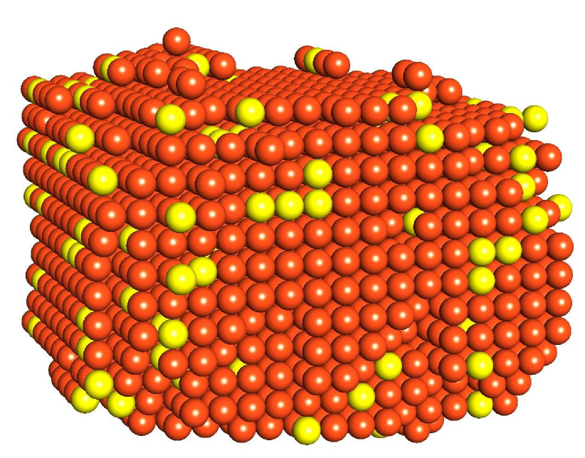
Figure 1: Precipitate obtained after the annealing during 1.2 s at 550°C of an aluminum solid solution containing 0.1 at.% Zr and 0.5 at.% Sc simulated with KMC (for clarity, only Zr and Sc atoms are shown). The corresponding radial concentration profile shows the Zr enrichment of the periphery compared to the core of the precipitate.

Figure 2: Projection in the plane $x_{\mathrm{Zr}}$, $n_{\mathrm{X}}$ of the precipitate distribution in a solid solution of composition $x^{0}_{\mathrm{Zr}}=0.5$ at.% and $x^{0}_{\mathrm{Sc}}=0.5$ at.% annealed at $T=550^{\circ}$C.

Following the composition and the size of all clusters present in the simulation box (Fig. 2), we see that small clusters, which should be sub-critical, can have all compositions between the two Al₃Zr and Al₃Sc stoichiometric compounds. As for over-critical clusters, the smaller ones are richer in Zr than the larger ones. These small clusters, which have just nucleated, grow by absorbing Sc atoms, leading to the tail of the distribution in the Sc richer part. As there is no diffusion inside precipitates (because of a high vacancy energy of formation and of the energetic cost associated with the creation of antisite defects), Zr and Sc atoms cannot homogenize. Therefore this distribution is consistent with the previous observation that the core of the precipitates can contain Zr whereas the intermediate shells contain almost exclusively Sc. This shows that Zr plays a role during nucleation but that growth is controlled by Sc, because this element diffuses much faster than Zr in the matrix. As precipitation is going on, the solid solution depletes in Sc. Therefore clusters can only grow by absorbing Zr atoms, leading to a move of the whole distribution towards the Zr richer part (Fig. 2). This is consistent with the fact that the external shells of the precipitates are richer in Zr. The precipitate growth by Zr absorption occurring in a second stage leads to a slowdown of the precipitation kinetics.

Figure 3: Kinetics of precipitation at $T=450^{\circ}$C: variation with the Zr and Sc concentration of the number $N_{p}$ of precipitates and of their mean size $<n_{\mathrm{X}}>$. The critical size to discriminate precipitates from sub-critical clusters is $n^{*}_{\mathrm{X}}=6$.

In agreement with TEM observations [1, 4], these atomic simulations show that a Zr addition to an Al-Sc alloy leads to a higher density of precipitates, these precipitates being smaller (Fig.3). Our atomic model allows to understand this effect. A Zr addition increases the nucleation driving force and thus the number of precipitates. As these ones mainly grow by absorbing Sc, one obtains smaller precipitates because the number of growing clusters is higher and there is less Sc available for growth at the end of the nucleation stage. The precipitate growth by Zr absorption is really slow but plays an important role too as it leads to the formation of an external Zr enriched shell which is responsible for the good resistance against coarsening. This kinetic effect due to the addition of an impurity having an attractive interaction with solute atoms ($\omega^{(2)}_{\mathrm{ZrSc}}<0$) has been already noticed by Soisson and Martin [22].

It is interesting to notice that a Sc addition to an Al-Zr alloy has quite distinct effects (Fig. 3). As Sc atoms plays a key role for nucleation and growth, such an addition leads to an increase of the precipitate density as well as to an increase of the precipitate size. Indeed the nucleation stage is shorter and the number of nucleating precipitates is higher. But this increase of the nuclei density does not consume the whole Sc in the solid solution and at the end of the nucleation stage, enough Sc remains so as to accelerate precipitate growth and coarsening, thus leading to bigger precipitates. In this case, one has to consider not only the thermodynamic contribution of the impurity addition, but its kinetic contribution too so as to conclude on its effects on the precipitation kinetics.

Cluster dynamics (CD)

KMC simulations allow us to understand precipitation kinetics in the ternary Al-Zr-Sc alloy in great details. Nevertheless, these simulations are restricted to short annealing times and high enough supersaturations, preventing any comparison with experimental data. Starting from the same atomic model, we build a mesoscopic modeling [23] which is based on a set of rate equations describing in the same framework the three different stages of precipitation, i.e. nucleation, growth and coarsening. It requires only a limited number of parameters, the interface free energy and the solute diffusion coefficients, which can be quite easily deduced from atomic parameters. The range of supersaturations and annealing times that can be simulated are thus extended for both binary Al-Zr and Al-Sc systems allowing a comparison with experimental data.

Mesoscopic model

In its strict sense, CD rests on the description of the alloy undergoing phase separation as a gas of solute clusters which exchange solute atoms by single atom diffusion[24, 25, 26]. Clusters are assumed to be spherical and are described by a single parameter, their size or the number $n_{\mathrm{X}}$ of solute atoms $\mathrm{X}$ they contain. In such a description, there is no precisely defined distinction between the solid solution on the one hand and the precipitates on the other hand, at variance with the CNT: the distribution of cluster sizes is the only quantity of interest (for a detailed discussion see Ref. 27).

Master equation.

The CD technique describes the precipitation kinetics thanks to a master equation giving the time evolution of the cluster size distribution[24, 25, 26]. When only monomers can migrate, which is the case for Al-Zr as well as Al-Sc systems [12], the probability $C_{n_{\mathrm{X}}}$ to observe a cluster containing $n_{\mathrm{X}}$ solute atoms obeys the differential equations

$$\frac{\mathrm{d}C_{n_{\mathrm{X}}}}{\mathrm{d}t} =J_{n_{\mathrm{X}}-1\to n_{\mathrm{X}}}-J_{n_{\mathrm{X}}\to n_{\mathrm{X}}+1},\quad\forall\ n_{\mathrm{X}}\geq 2$$ (4a)

$$\frac{\mathrm{d}C_{1}}{\mathrm{d}t} =-2J_{1\to 2}-\sum_{n_{\mathrm{X}}\geq 2}{J_{n_{\mathrm{X}}\to n_{\mathrm{X}}+1}},$$ (4b)

where the flux $J_{{n_{\mathrm{X}}}\to{n_{\mathrm{X}}}+1}$ from the class of size $n_{\mathrm{X}}$ to the class $n_{\mathrm{X}}+1$ is written

$$J_{{n_{\mathrm{X}}}\to{n_{\mathrm{X}}}+1}=\beta_{n_{\mathrm{X}}}C_{n_{\mathrm{X}}}-\alpha_{{n_{\mathrm{X}}}+1}C_{{n_{\mathrm{X}}}+1},$$ (5)

$\beta_{n_{\mathrm{X}}}$ being the probability per unit time for one solute atom to impinge on a cluster of size $n_{\mathrm{X}}$ and $\alpha_{n_{\mathrm{X}}}$ for one atom to leave a cluster of size $n_{\mathrm{X}}$.

Condensation rate.

When the solute long-range diffusion controls the precipitation kinetics, the condensation rate is obtained by solving the diffusion problem in the solid solution around a spherical precipitate. For a cluster of radius $r_{n_{\mathrm{X}}}$, this condensation rate takes the form [28, 29]

$$\beta_{n_{\mathrm{X}}}=4\pi r_{n_{\mathrm{X}}}\frac{D_{\mathrm{X}}}{\Omega}C_{1},$$ (6)

where $D_{\mathrm{X}}$ is the diffusion coefficient of the solute at infinite dilution of the solid solution and $\Omega$ is the mean atomic volume corresponding to one lattice site.

Evaporation rate.

The evaporation rate is obtained assuming that it is an intrinsic property of the cluster and therefore does not depend on the solid solution surrounding the cluster. This means that the cluster has enough time to explore all its configurations between the arrival and the departure of a solute atom. Thus $\alpha_{n_{\mathrm{X}}}$ should not depend on the nominal concentration of the solid solution and can be obtained by considering any undersaturated solid solution of nominal concentration $x^{0}_{\mathrm{X}}$. Such a solid solution is stable. Then there should be no energy dissipation. This involves that all fluxes $J_{n_{\mathrm{X}}\to n_{\mathrm{X}}+1}$ equal zero. Using equation 5, one obtains

$$\alpha_{{n_{\mathrm{X}}}+1}=\bar{\alpha}_{{n_{\mathrm{X}}}+1}(x^{0}_{\mathrm{X}})=\bar{\beta}_{n_{\mathrm{X}}}(x^{0}_{\mathrm{X}})\frac{\bar{C}_{n_{\mathrm{X}}}(x^{0}_{\mathrm{X}})}{\bar{C}_{{n_{\mathrm{X}}}+1}(x^{0}_{\mathrm{X}})},$$ (7)

where overlined quantities are evaluated in the solid solution at equilibrium. This finally leads to

$$\alpha_{{n_{\mathrm{X}}}+1}=4\pi r_{n_{\mathrm{X}}}\frac{D_{\mathrm{X}}}{\Omega}\exp{\left[(G_{n_{\mathrm{X}}+1}-G_{n_{\mathrm{X}}}-G_{1})/kT\right]},$$ (8)

where $G_{n_{\mathrm{X}}}$ is the free energy of a cluster containing $n_{\mathrm{X}}$ atoms. It can be divided into a volume and an interface contributions, which involves the following expression of the evaporation rate:

$$\alpha_{{n_{\mathrm{X}}}+1}=4\pi r_{n_{\mathrm{X}}}\frac{D_{\mathrm{X}}}{\Omega}\exp{\left[(36\pi)^{1/3}a^{2}\left((n_{\mathrm{X}}+1)^{2/3}\sigma_{n_{\mathrm{X}}+1}-{n_{\mathrm{X}}}^{2/3}\sigma_{n_{\mathrm{X}}}-\sigma_{1}\right)/kT\right]},$$ (9)

where $\sigma_{n_{\mathrm{X}}}$ is the interface free energy of a cluster containing $n_{\mathrm{X}}$ solute atoms and $a$ the lattice parameter.

Looking at the expression 6 of the condensation rate and the expression 9 of the evaporation rate, one sees that the only parameters needed by CD are the diffusion coefficient and the interface free energy. There is no need to know the nucleation free energy in opposition to other mesoscopic models based on CNT. In CD, thermodynamics of the solid solution is described thanks to a lattice gas model and therefore the nucleation free energy results from this description and is not an input of the modeling.

Interface free energy.

The interface free energy can be deduced from the atomic model [12] by computing within the Bragg-Williams approximation the free energies corresponding to planar interfaces between the aluminum solid solution and the L1₂ precipitates for the three most dense packing orientations {111}, {110} and {100}. We obtain $\sigma_{100}<\sigma_{110}<\sigma_{111}$, indicating that precipitates mainly show facets in the {100} direction and that facets in the {110} and {111} directions are small. As the difference between $\sigma_{100}$, $\sigma_{110}$ and $\sigma_{111}$ is decreasing with temperature, precipitates are becoming more isotropic at higher temperatures. This is in agreement with the shapes of the precipitates observed during the atomic simulations, as well as with experimental observations done by Marquis and Seidman [30].

So as to get the input parameters needed by CD, one has to deduce an isotropic average interface free energy $\bar{\sigma}$ from these planar interface free energies. This can be done using the Wulff construction [31, 32]: $\bar{\sigma}$ is defined so as to give the same interface free energy for a spherical precipitate having the same volume as the real faceted one. For temperatures ranging between 0 K and the aluminum melting temperature (933.5 K), $\bar{\sigma}$ is varying between 124 and 92 mJ.m^-2 for Al₃Zr precipitates and between 138 and 95 mJ.m^-2 for Al₃Sc precipitates.

Figure 4: Variation with the cluster size $n_{\mathrm{Sc}}$ of the interface free energy between the solid solution and Al₃Sc at three different temperatures (300, 400, and 500^∘C). Symbols correspond to $\sigma_{n_{\mathrm{Sc}}}$ as given by the direct calculation of the cluster formation free energy (Eq. 20 of Ref. 12) and lines to the capillary approximation (Eq. 10) as well as to its asymptotic limit. Dotted lines indicate the range of sizes where the coefficients $c$ and $d$ have been fitted.

The interface free energy $\bar{\sigma}$ does not depend on the size of the cluster and corresponds to the asymptotic limit of the quantity $\sigma_{n_{\mathrm{X}}}$ used to define the evaporation rate (Eq. 9). A direct calculation considering the partition functions of small clusters [12] shows that $\sigma_{n_{\mathrm{X}}}$ slightly deviates from this asymptotic value at small sizes (Fig. 4). Nevertheless, CD is very sensitive to this input parameter because its thermodynamic description only relies on it. Therefore, the size dependence of $\sigma_{n_{\mathrm{X}}}$ has to be considered. In this purpose, for clusters containing no more than 9 solute atoms, the interface free energy is computed precisely using Eq. 20 of Ref. 12 and for clusters of size $n_{\mathrm{X}}\geq 10$, the interface free energy is obtained using an extension of the capillary approximation,

$$\sigma_{n_{\mathrm{X}}}=\bar{\sigma}\left(1+c\ n_{\mathrm{X}}^{-1/3}+d\ n_{\mathrm{X}}^{-2/3}\right),$$ (10)

where $c$ and $d$ respectively correspond to the line and point contributions [33]. The asymptotic value $\bar{\sigma}$ used is the one previously calculated whereas coefficients $c$ and $d$ are obtained by a least square fit of the exact expression for sizes $5\geq n_{\mathrm{X}}\geq 9$.

Precipitation kinetics

Figure 5: Mean precipitate radius and precipitate density as a function of the aging time for a solid solution of composition $x^{0}_{\mathrm{Sc}}=0.18$ at.% at different temperatures ($T=300$, 350, and 400°C) as given by CD and compared to experimental data[34, 30, 35, 36] and to KMC results[12]. The cutoff radius used for CD and KMC is $r^{*}\sim 0.75$ nm ($n_{\mathrm{X}}^{*}=27$).

In order to compare precipitation kinetics obtained from KMC and from CD simulations, an arbitrary threshold size $n_{\mathrm{X}}^{*}$ is used to define precipitates so as to be able to calculate mean quantities like the precipitate size and density. Below this threshold size, clusters are assumed to be invisible. When comparing with experimental data, we choose $n_{\mathrm{X}}^{*}=27$ corresponding to a precipitate diameter equal to 1.5 nm which is supposed to be the smallest size which can be discriminated by TEM. This threshold size can thus be different from the critical size of CNT: the only important thing is to use the same criterion to define precipitates when comparing atomic and mesoscopic simulations.

Comparing the precipitation kinetics obtained with KMC and CD simulations, one sees that CD manages to reproduce the variations of the precipitate density and of their mean size (Fig. 5). A more thorough comparison [23] shows that CD catches variations with the supersaturations and the annealing temperatures of the precipitation kinetics. For low supersaturations, the agreement between both modeling is really good, whereas for high supersaturations, kinetics modeled by CD appear to be slightly too slow compared to the ones simulated with KMC. This delay only corresponds to a constant factor on the time scale and in all cases the prediction of the precipitate maximal density at the transition between the growth and the coarsening stages is correct.

Precipitation kinetics simulated with CD can be compared too with the experimental data of Novotny and Ardell [34] and those of Marquis et al. [30, 35, 36] who studied an aluminum alloy having the composition $x^{0}_{\mathrm{Sc}}=0.18$ at.%. For the three different temperatures $T=300$, $350$ and $400^{\circ}$C, it appears that the CD equations manage to reproduce the variation with time of the mean precipitate radius (Fig. 5). Despite the fact that the time scales in real experiments are several order of magnitude larger than those in KMC, CD, with a single set of parameters, reproduces atomic simulations at short times and gives a safe extrapolation thereof to the range of annealing times that can be compared with experimental data. In Ref. 23, it was shown too that the precipitate size distributions simulated with CD agrees really well with the experimentally ones measured by Novotny and Ardell [34].

Figure 6: Time evolution of the resistivity $\rho$ experimentally observed [37, 38] and deduced from CD simulations for two solid solution of composition $x^{0}_{\mathrm{Sc}}=0.12$ and 0.24 at.%.

CD can be used so as to simulate the evolution of the electric resistivity during annealing kinetics. Some calculations of the electrical resistivity associated with a cluster distribution exist in the literature [39, 40], but as a first approximation, one can consider that the resistivity contribution $\rho_{n}$ of a cluster of size $n$ is proportional to its section, $\rho_{n}=\rho_{1}n^{2/3}$. If one assumes that all clusters are contributing to the resistivity, the resistivity measured at time $t$ in the phase separating system should be

$$\rho(t)=\rho^{0}_{\mathrm{Al}}+\delta\rho_{\mathrm{Sc}}\sum_{n=1}^{\infty}{C_{n}(t)n^{2/3}},$$ (11)

where the size distribution $C_{n}(t)$ is given by CD (Eq. 4). $\rho^{0}_{\mathrm{Al}}$ is the resistivity of pure aluminum and is temperature dependent. The increase of resistivity with Sc content has been measured at 77 K by Fujikawa et al. [41, 42] who give $\delta\rho_{\mathrm{Sc}}=3400$ n$\Omega$m. Assuming that Matthienssen rule[43] is obeyed, this quantity does not depend on the temperature. When comparing resistivity predicted by CD with the experimental ones measured during precipitation kinetics [37, 38] we obtain a good agreement (Fig. 6), especially for the lowest temperatures: CD manages to reproduce the fast decrease of resistivity during the nucleation and growth stages as well as the slower variation which follows during the coarsening stage. For the highest temperatures (330^∘C for the solid solution of concentration $x^{0}_{\mathrm{Sc}}=0.12$ at.% and 400°C for $x^{0}_{\mathrm{Sc}}=0.24$ at.%), CD appears to be too fast compared to experimental data. This may arise from the approximation we are using for the contributions to resistivity of the various clusters as this size dependence may be too crude for small clusters. One should notice too that the evolution predicted by CD at these temperatures is really fast and that the resistivity drop appears at times ($t\sim 10$ s) which are too small to be precisely observed experimentally.

CD is thus a powerful modeling technique to study precipitation in a binary alloy, allowing to link different scales. Starting from an atomic diffusion model, it gives quantitative predictions of precipitation kinetics in agreement with experimental data. It is possible to generalize this mesoscopic technique so as to study precipitation in a ternary alloy[44] but some work still needs to be done. In the case of the Al-Zr-Sc alloy, one of the main difficulties is to find a way for CD to describe the precipitate inhomogeneities. Therefore, in the following, we will not use this technique to model the whole kinetics of precipitation in the ternary alloy, but we will focus on the nucleation stage and see how CNT can be extended so as to predict the nucleation rate as well as the compositions $x$ of the Al₃Zr_xSc_1-x nuclei in this ternary alloy.

Classical nucleation theory (CNT)

CNT allows to predict the nucleation rate in a supersaturated binary solid solution. Comparisons with KMC simulations [47, 48, 49, 22, 50, 51, 12] show that its predictions are correct as long as its input parameters are carefully evaluated. In particular, for the Al-Zr and Al-Sc alloys, it has been shown that one has to take into account the ordering tendency of the binary alloy when calculating the nucleation driving force[12]. We will see how this can be done in a convenient way as well as how CNT applies to the two binary Al-Zr and Al-Sc alloys, before extending the theory to the ternary Al-Zr-Sc alloy.

Binary Al-Zr and Al-Sc alloys

Whereas CD describes the time evolution of the whole cluster size distribution (Eq. 4), CNT assumes that the distribution is stationary in the solid solution, i.e. below a critical size $n_{\mathrm{X}}^{*}$, and does not provide any information on the distribution of larger clusters. The probability to observe a cluster containing $n_{\mathrm{X}}$ solute atoms for $n_{\mathrm{X}}\leq n_{\mathrm{X}}^{*}$ is thus given by

$$C_{n_{\mathrm{X}}}=\exp{\left(-\Delta G_{n_{\mathrm{X}}}/kT\right)},$$ (12)

where $\Delta G_{n_{\mathrm{X}}}$ is the formation free energy of the cluster. It can be evaluated thanks to the capillary approximation, dividing this formation free energy into a volume and a surface contribution,

$$\Delta G_{n_{\mathrm{X}}}(x_{\mathrm{X}}^{0})=4n_{\mathrm{X}}\Delta G^{nuc}(x_{\mathrm{X}}^{0})+\left(36\pi\right)^{1/3}{n_{\mathrm{X}}}^{2/3}a^{2}\sigma_{n_{\mathrm{X}}}.$$ (13)

One thus sees that CNT needs one more input parameter than CD, the nucleation free energy $\Delta G^{nuc}(x_{\mathrm{X}}^{0})$.

With this additional parameter and the assumption on the cluster size distribution in the metastable solid solution, CNT leads to the following prediction of the steady-state nucleation rate,

$$J^{st}=4N_{s}\beta_{n_{\mathrm{X}}^{*}}\sqrt{-\frac{1}{2\pi kT}\left.\frac{\partial^{2}{\Delta G_{n_{\mathrm{X}}}}}{\partial{n_{\mathrm{X}}}^{2}}\right|_{n_{\mathrm{X}}=n_{\mathrm{X}}^{*}}}\exp{\left(-\frac{\Delta G_{n_{\mathrm{X}}*}}{kT}\right)},$$ (14)

where $N_{s}$ is the number of lattice site. The condensation rate $\beta_{n_{\mathrm{X}}^{*}}$ takes the same expression as in CD (Eq. 6) and, like the formation free energy and its second derivative, it is evaluated for the critical size $n_{\mathrm{X}}^{*}$ corresponding to the maximum of the formation free energy.

Figure 7: Variation with the nominal concentration and the temperature of the steady-state nucleation rate $J^{st}$ for Al₃Zr precipitation. Symbols correspond to KMC simulations and lines to CNT. On the left, different thermodynamic approximations are used to evaluate $\Delta G^{nuc}$: the ideal and regular solid solution models, the cluster variation method (CVM) and the low temperature expansion (LTE) to second order (Eq. 15). On the right, only LTE is used.

Different thermodynamic approximations can be used to obtain the nucleation free energy from the atomic model. Usually, one uses simple mean-field approximation, like the ideal or regular solid solution model which both rely on the Bragg-Williams approximation. Nevertheless, we showed in Ref. 12 that they lead to bad predictions of the CNT: the cluster size distribution in the solid solution corresponding to Eq. 12 completely disagrees with that observed during KMC simulations. As the steady-state nucleation rate relies on this distribution, we observe the same discrepancy for the prediction of $J^{st}$ (Fig. 7). So as to obtain a good agreement, one has to take into account order effects corresponding to the strong attraction existing between Al and Zr as well as Al and Sc atoms when they are first nearest neighbors and the strong repulsion when they are second nearest neighbors This can be done using the cluster variation method (CVM) [52, 53] to calculate the nucleation free energy. The cluster size distribution given by Eq. 12 then corresponds to the one observed in atomic simulations and CNT theory well reproduces the nucleation rate (Ref. 12 and Fig. 7). Nevertheless, one drawback of CVM is that it does not lead to an analytical expression of the nucleation free energy. It is then not really convenient to combine it with a theory whose main contribution is to give an analytical expression of the nucleation rate. Moreover, it would be interesting to understand thoroughly what is wrong with the ideal and the regular solid solution models and in particular why the regular model leads to worse predictions than the ideal one. In this purpose, we use low temperature expansions[54]. This thermodynamic approximation leads to analytical expression of the nucleation free energy and takes correctly into account the ordering tendency of the alloy.

A low temperature expansion consists in developing the partition function of the system around a reference state, keeping in the series only the excited states of lowest energies. For an Al-Sc or an Al-Zr solid solution, this reference state corresponds to pure Al and the two first excited states are the transformation of an Al atom into an X solute atom and of a pair of Al second nearest neighbors to a pair of X atoms. When considering only the second order of the expansion, one can obtain analytical expressions of the different thermodynamic quantities in the canonic ensemble, thus depending on the nominal concentration $x_{\mathrm{X}}^{0}$ of the solid solution. In particular, the nucleation free energy takes the form

$$\begin{split}\Delta G^{nuc}(x_{\mathrm{X}}^{0})=&kT\left[\operatorname{q}{(x_{\mathrm{X}}^{0})}-\operatorname{q}{(x_{\mathrm{X}}^{eq})}\right]+3kT\exp{\left(2\omega^{(2)}_{\mathrm{AlX}}/kT\right)}\left[\operatorname{q}{(x_{\mathrm{X}}^{0})}^{2}-\operatorname{q}{(x_{\mathrm{X}}^{eq})^{2}}\right]\\ &-\frac{1}{4}kT\left\{\ln{\left[\operatorname{q}{(x_{\mathrm{X}}^{0})}\right]}-\ln{\left[\operatorname{q}{(x_{\mathrm{X}}^{eq})}\right]}\right\},\end{split}$$ (15)

where we have defined the function

$$\operatorname{q}{(x)}=\frac{2x}{1+\sqrt{1+24x\exp{\left(2\omega^{(2)}_{\mathrm{AlX}}/kT\right)}}}.$$ (16)

Using this expression of the nucleation free energy with CNT one obtains predictions of the nucleation rate as good as with CVM (Fig. 7) compared to the rate observed during KMC simulations. In particular, the variations with the concentration of the solid solution and with the annealing temperatures are well reproduced.

So as to understand why simple mean-field approximations lead to bad approximations of the nucleation free energy, we develop the expression 15 to first order in the concentrations $x_{\mathrm{X}}^{0}$ and $x_{\mathrm{X}}^{eq}$:

$$\Delta G^{nuc}_{LTE}(x_{\mathrm{X}}^{0})\sim\frac{3}{4}kT\ln{\left(\frac{1-x_{\mathrm{X}}^{eq}}{1-x_{\mathrm{X}}^{0}}\right)}+\frac{1}{4}kT\ln{\left(\frac{x_{\mathrm{X}}^{eq}}{x_{\mathrm{X}}^{0}}\right)}+\frac{1}{4}\left(1+6\mathrm{e}^{2\omega^{(2)}_{\mathrm{AlX}}/kT}\right)\left(x_{\mathrm{X}}^{0}-x_{\mathrm{X}}^{eq}\right).$$ (17)

Doing the same development for the nucleation free energy calculated within the Bragg-Williams approximation (regular solid solution), we obtain

$$\Delta G^{nuc}_{reg}(x_{\mathrm{X}}^{0})\sim\frac{3}{4}kT\ln{\left(\frac{1-x_{\mathrm{X}}^{eq}}{1-x_{\mathrm{X}}^{0}}\right)}+\frac{1}{4}kT\ln{\left(\frac{x_{\mathrm{X}}^{eq}}{x_{\mathrm{X}}^{0}}\right)}+\left(6\omega^{(1)}_{\mathrm{AlX}}+3\omega^{(2)}_{\mathrm{AlX}}\right)\left(x_{\mathrm{X}}^{0}-x_{\mathrm{X}}^{eq}\right).$$ (18)

Comparing Eq. 17 with Eq. 18, we see that these two thermodynamic approximations deviate from the ideal solid solution model by a distinct linear term. In the low temperature expansion (Eq. 17), the nucleation free energy is only depending on the second nearest neighbor interaction and the coefficient in front of the concentration is positive. On the other hand, the Bragg-Williams approximation (Eq. 18) incorporates both first and second nearest neighbor interactions into a global parameter $\omega_{\mathrm{AlX}}=6\omega^{(1)}_{\mathrm{AlX}}+3\omega^{(2)}_{\mathrm{AlX}}$. This leads to a linear correction with a negative coefficient as $\omega_{\mathrm{AlX}}<0$ for both binary alloys. We thus demonstrate that the regular solid solution model leads to a wrong correction of the ideal model because it does not consider properly short range order. In the case of a L1₂ ordered compound precipitating from a solid solution lying on a fcc lattice, one cannot use such an approximation to calculate the nucleation free energy. On the other hand, Eq. 15 is a good approximation and can be used to calculate the nucleation free energy even when the second nearest neighbor interaction $\omega^{(2)}_{\mathrm{AlX}}$ is not known. Indeed, this parameter can be deduced from the solubility limit $x_{\mathrm{X}}^{eq}$ by inverting Eq. 4 of Ref. [12], leading to the relation

$$\omega^{(2)}_{\mathrm{AlX}}=-\frac{1}{6}kT\ln{\left(x_{\mathrm{X}}^{eq}\right)}+kT\left({x_{\mathrm{X}}^{eq}}^{2/3}+\frac{49}{6}{x_{\mathrm{X}}^{eq}}^{4/3}\right).$$ (19)

This relation combined with Eq. 15 provides a powerful way for calculating the nucleation free energy from the solid solubility.

Ternary Al-Zr-Sc alloy

We now explore how CNT can be extended to the Al-Zr-Sc alloy. Going from the binary to the ternary alloy, the main difficulty is that the precipitates have the composition Al₃Zr_xSc_1-x, where $x$ is not known a priori. Therefore, the theory has to predict their composition. As we showed for the two binary Al-Zr and Al-Sc alloys that the capillary approximation is well suited to describe thermodynamics of the clusters, even the smallest ones, We use the same approximation for the ternary system. The formation free energy of a cluster Al₃Zr_xSc_1-x containing $n_{\mathrm{X}}$ solute atoms can then be written

$$\Delta G_{n_{\mathrm{X}}}(x^{0}_{\mathrm{Zr}},x^{0}_{\mathrm{Sc}},x)=4n_{\mathrm{X}}\Delta G^{nuc}(x^{0}_{\mathrm{Zr}},x^{0}_{\mathrm{Sc}},x)+\left(36\pi\right)^{1/3}{n_{\mathrm{X}}}^{2/3}a^{2}\bar{\sigma}(x).$$ (20)

The nucleation free energy is depending not only on the composition of the supersaturated solid solution but also on the composition of the nucleus:

$$\begin{split}\Delta G^{nuc}(x^{0}_{\mathrm{Zr}},x^{0}_{\mathrm{Sc}},x)=&\frac{1}{4}\left\{x\left[3\mu_{\mathrm{Al}}^{p}(x)+\mu_{\mathrm{Zr}}^{p}(x)\right]+(1-x)\left[3\mu_{\mathrm{Al}}^{p}(x)+\mu_{\mathrm{Sc}}^{p}(x)\right]\right.\\ &-x\left[3\mu_{\mathrm{Al}}^{ss}(x^{0}_{\mathrm{Zr}},x^{0}_{\mathrm{Sc}})+\mu_{\mathrm{Zr}}^{ss}(x^{0}_{\mathrm{Zr}},x^{0}_{\mathrm{Sc}})\right]\\ &\left.-(1-x)\left[3\mu_{\mathrm{Al}}^{ss}(x^{0}_{\mathrm{Zr}},x^{0}_{\mathrm{Sc}})+\mu_{\mathrm{Sc}}^{ss}(x^{0}_{\mathrm{Zr}},x^{0}_{\mathrm{Sc}})\right]\right\}.\end{split}$$ (21)

$\mu_{\mathrm{Al}}^{ss}$, $\mu_{\mathrm{Sc}}^{ss}$ and $\mu_{\mathrm{Zr}}^{ss}$ are the chemical potentials in the solid solution: we use a low temperature expansion to the second order to calculate them. $\mu_{\mathrm{Al}}^{p}$, $\mu_{\mathrm{Sc}}^{p}$ and $\mu_{\mathrm{Zr}}^{p}$ are the chemical potentials in the precipitate. The thermodynamic approach used to calculate them mixes low temperature expansion so as to correctly describe the majority sublattice which only contains Al atoms as well as Bragg-Williams approximation because of the minority sublattice which can equally be occupied by Zr or Sc atoms. This approach ensures that for $x=0$ or 1, Eq. 21 leads to the same value for the nucleation free energy as the calculation in the corresponding binary alloy (Eq. 15).

As the two binary Al₃Zr and Al₃Sc compounds have a close interface free energy and as the interaction parameter $\omega^{(2)}_{\mathrm{ZrSc}}$ is low in magnitude, we assume a linear interpolation to calculate the interface free energy of the Al₃Zr_xSc_1-x compound,

$$\bar{\sigma}(x)=x\bar{\sigma}(\mathrm{Al}_{3}\mathrm{Zr})+(1-x)\bar{\sigma}(\mathrm{Al}_{3}\mathrm{Sc}).$$ (22)

CNT is not as sensitive as CD to this parameter because not all the thermodynamics is based on it. Therefore, one does not need to consider the size dependence of the interface free energy as we did for CD.

Figure 8: Size distribution of Al₃Zr_xSc_1-x clusters depending on their number $n_{\mathrm{Zr}}$ and $n_{\mathrm{Sc}}$ of atoms for a solid solution of concentration $x^{0}_{\mathrm{Zr}}=0.1$  at.% and $x^{0}_{\mathrm{Sc}}=0.5$ at.% at $T=550^{\circ}$C. Symbols correspond to KMC simulations and lines to predictions of CNT.

The cluster size distribution in the metastable solid solution still obeys Eq. 12 where now the cluster free energy is depending on the cluster composition and is given by Eq. 20. Comparing this distribution with the one observed during KMC simulations (Fig. 8), we obtain a satisfactory agreement showing that our thermodynamic description of the cluster assembly is correct.

Figure 9: Variation with the composition $x$ of the Al₃Zr_xSc_1-x nucleus of the critical size $n_{\mathrm{X}}^{*}$ (Eq 24), the free energy $\Delta G^{*}$ of the critical nucleus, the Zeldovitch factor $Z$ (Eq. 26), the condensation rate $\beta^{*}$ (Eq. 27) and the nucleation rate $J^{st}$ (Eq. 25) for a solid solution of concentration $x^{0}_{\mathrm{Zr}}=0.1$  at.% and $x^{0}_{\mathrm{Sc}}=0.5$ at.% at $T=550^{\circ}$C.

So as to define a classical nucleation rate we use the fact that Sc diffuses faster than Zr. We therefore assume that any critical nucleus is growing by absorbing a Sc atom and we neglect Zr absorption. A critical size can then be defined for each set of clusters containing the same number $n_{\mathrm{Zr}}$ of Zr atoms. This critical size corresponds to the maximum of the cluster free energy (Eq. 20) with $n_{\mathrm{Zr}}$ being fixed and is thus given by the condition

$$\left(\frac{\partial{\Delta G_{n_{\mathrm{X}}}(x)}}{\partial{n_{\mathrm{Sc}}}}\right)_{n_{\mathrm{Zr}}}=0.$$ (23)

This leads to a critical size depending on the composition $x$ of the cluster,

$$n^{*}(x)=4n_{\mathrm{X}}^{*}(x)=\frac{16\pi}{3}\left(\frac{(2+x)\ a^{2}\bar{\sigma}(\mathrm{Al}_{3}\mathrm{Sc})-x\ a^{2}\bar{\sigma}(\mathrm{Al}_{3}\mathrm{Zr})}{\mu_{\mathrm{Sc}}^{ss}+3\ \mu_{\mathrm{Al}}^{ss}-\mu_{\mathrm{Sc}}^{p}(x)-3\ \mu_{\mathrm{Al}}^{p}(x)}\right)^{3}.$$ (24)

We can define now a nucleation rate $J^{st}(x)$ depending on the composition of the nucleus. As in the binary alloy, this rate takes the form

$$J^{st}(x)=N_{s}\ Z(x)\ \beta^{*}(x)\ \exp{\left(-\Delta G^{*}(x)/kT\right)}.$$ (25)

The Zeldovitch factor $Z(x)$ is defined along the destabilization direction of the nucleus and is thus obtained by considering the second derivative of the nucleus free energy with respect to $n_{\mathrm{Sc}}$, keeping $n_{\mathrm{Zr}}$ constant:

$$Z(x)=4\sqrt{-\frac{1}{32\pi kT}\left(\frac{\partial^{2}{\Delta G_{n}}}{\partial{n_{\mathrm{Sc}}}^{2}}\right)_{n_{\mathrm{Zr}}}}.$$ (26)

$\Delta G^{*}(x)$ is the cluster free energy (Eq. 20) of a cluster having the critical size $n_{\mathrm{X}}^{*}(x)$. As for the condensation rate, it is obtained by considering the absorption of Sc atoms by the critical nucleus, leading to

$$\beta^{*}(x)=8\pi\left(\frac{3n_{\mathrm{X}}^{*}(x)}{2\pi}\right)^{1/3}\frac{D_{\mathrm{Sc}}}{a^{2}}\frac{x^{0}_{\mathrm{Sc}}}{1-x}.$$ (27)

Writing the nucleation rate in this way, we ensure that when $x=0$ we obtain the same expression as that given by CNT in the Al-Sc alloy (Eq. 14).

Figure 10: Variation of the nucleation rate $J^{st}$ (Maximum of $J^{st}(x)$ given by Eq. 25) with the zirconium concentration for different scandium concentrations of the solid solution and different annealing temperatures.

The variations of the nucleation rate $J^{st}(x)$ with the composition $x$ of the nucleus are shown in Fig. 9 for a chosen supersaturated solid solution. So as to compare results of this nucleation model with KMC simulations, we define the nucleation rate $J^{st}$ as the maximum of the function $J^{st}(x)$ given by Eq. 25. The critical size used to extract the nucleation rate from KMC simulations is the one corresponding to this maximum. When the solid solution is highly supersaturated in Sc ($x^{0}_{\mathrm{Sc}}=0.5$ at.% at $T=450$ of $550^{\circ}$), our mesoscopic models reproduces the variation of the nucleation rate with the zirconium concentration of the solid solution (Fig. 10). The mesoscopic evaluation of $J^{st}$ worsens a little bit when the Zr concentration becomes comparable to the Sc one and when the Sc supersaturation becomes lower. Nevertheless, the key point is that this extension of CNT manages to predict the increase of the nucleation rate with a Zr addition to an Al-Sc alloy, this increase being in reasonable agreement with atomic simulations. More advanced models (e.g. the link flux analysis and other approximations as described in Ref. [56, 57, 58]) are worth to be tried.

Conclusions

This study illustrates how a quantitative multiscale modeling of the precipitation kinetics can be performed. Using a very limited number of input data, we built for the Al-Zr-Sc alloy an atomic model from which mesoscopic quantities like the interface free energy or the nucleation free energy could be deduced. For the two binary Al-Zr and Al-Sc alloys, it was shown that a good agreement can be obtained between the KMC simulations, different mesoscopic models (CD and CNT) and experimental data. So as to obtain good predictions with CNT, one has to take into account the ordering tendency of the system. In this purpose, using low temperature expansions, we propose an analytical expression of the nucleation free energy. For the ternary Al-Zr-Sc alloy, we showed that the precipitate inhomogeneity arises from the difference between the two solute diffusion coefficients. Although the precipitate composition is not known a priori, CNT could be extended to this ternary alloy thanks to reasonable assumptions on the kinetics. This mesoscopic model reproduces the increase of the nucleation rate associated with a Zr addition to an Al-Sc alloy.

References

- [1] V. I. Yelagin, V. V. Zakharov, S. G. Pavlenko, and T. D. Rostova. “Influence of Zirconium Additions on Ageing of Al-Sc Alloys.” Phys. Met. Metall., 60 (1985), 88–92
- [2] V. G. Davydov, V. I. Yelagin, V. V. Zakharov, and T. D. Rostova. “Alloying Aluminum Alloys with Scandium and Zirconium Additives.” Metal Science and Heat Treatment, 38 (1996), 347–352
- [3] L. S. Toropova, D. G. Eskin, M. L. Kharaterova, and T. V. Bobatkina. Advanced Aluminum Alloys Containing Scandium - Structure and Properties (Amsterdam: Gordon and Breach Sciences, 1998)
- [4] C. B. Fuller, D. N. Seidman, and D. C. Dunand. “Mechanical Properties of Al(Sc,Zr) Alloys at Ambient and Elevated Temperatures.” Acta Mater., 51 (2003), 4803–4814
- [5] Y. W. Riddle and T. H. Sanders. “A Study of Coarsening, Recrystallization, and Morphology of Microstructure in Al-Sc-(Zr)-(Mg) Alloys.” Metall. Mater. Trans. A, 35 (2004), 341–350
- [6] J. Røyset and N. Ryum. “Scandium in Aluminium Alloys.” Int. Mater. Rev., 50 (2005), 19–44
- [7] P. Villars and L. D. Calvert. Pearson’s Handbook of Crystallographic Data for Intermetallic Phases (Oh: American Society for Metals, 1985)
- [8] Y. Harada and D. C. Dunand. “Microstructure of Al3Sc with Ternary Transition-Metal Additions.” Mater. Sci. Eng., A329–331 (2002), 686–695
- [9] J. D. Robson and P. B. Prangnell. “Dispersoid Precipitation and Process Modelling in Zirconium Containing Commercial Aluminium Alloys.” Acta Mater., 49 (2001), 599–613
- [10] N. Ryum. “Precipitation and Recrystallization in an Al-0.5 wt.% Zr Alloy.” Acta Metall., 17 (1969), 269–278
- [11] E. Nes. “Precipitation of the Metastable Cubic Al3Zr-Phase in Subperitectic Al-Zr Alloys.” Acta Metall., 20 (1972), 499–506
- [12] E. Clouet, M. Nastar, and C. Sigli. “Nucleation of Al3Zr and Al3Sc in Aluminum Alloys: from Kinetic Monte Carlo Simulations to Classical Theory.” Phys. Rev. B, 69 (2004), 064109
- [13] E. Clouet, J. M. Sanchez, and C. Sigli. “First-Principles Study of the Solubility of Zr in Al.” Phys. Rev. B, 65 (2002), 094105
- [14] M. Methfessel and M. van Schilfgaarde. “Derivation of Force Theorem in Density-Functional Theory: Application to the Full-Potential LMTO Method.” Phys. Rev. B, 48 (1993), 4937–4940
- [15] J. P. Perdew, K. Burke, and M. Ernzerhof. “Generalized Gradient Approximation Made Simple.” Phys. Rev. Lett., 77 (1996), 3865–3868
- [16] J. W. Connolly and A. R. Williams. “Density-Functional Theory Applied to Phase Transformations in Transition-Metal Alloys.” Phys. Rev. B, 27 (1983), 5169–5172
- [17] L. S. Toropova, A. N. Kamardinkin, V. V. Kindzhibalo, and A. T. Tyvanchuk. “Investigation of Alloys of the Al-Sc-Zr System in the Aluminium-Rich Range.” Phys. Met. Metall., 70 (1990), 106–110
- [18] A. Tolley, V. Radmilovic, and U. Dahmen. “Segregation in Al3(Sc,Zr) Precipitates in Al-Sc-Zr Alloys.” Scripta Mater., 52 (2005), 621–625
- [19] V. Radmilovic, A. Tolley, and U. Dahmen. “Precipitate Evolution and Coarsening Kinetics in Al-Sc-Zr Alloys.” In “Solid-Solid Phase Transformations in Inorganic Materials,” (TMS, 2005)
- [20] B. Forbord, W. Lefebvre, F. Danoix, H. Hallem, and K. Marthinsen. “Three Dimensional Atom Probe Investigation on the Formation of Al3(Sc,Zr)-Dispersoids in Aluminium Alloys.” Scripta Mater., 51 (2004), 333–337
- [21] C. B. Fuller, J. L. Murray, and D. N. Seidman. “Temporal Evolution of the Nanostructure of Al(Sc,Zr) Alloys: Part I-Chemical Compositions of Al3(Sc1-xZrx) Precipitates.” Acta Mater., submitted (2005)
- [22] F. Soisson and G. Martin. “Monte-Carlo Simulations of the Decomposition of Metastable Solid Solutions: Transient and Steady-State Nucleation Kinetics.” Phys. Rev. B, 62 (2000), 203–214
- [23] E. Clouet, A. Barbu, L. Laé, and G. Martin. “Precipitation Kinetics of Al3Zr and Al3Sc in Aluminum Alloys Modeled with Cluster Dynamics.” Acta Mater., 53 (2005), 2313–2325
- [24] S. I. Golubov, Y. N. Osetsky, A. Serra, and A. V. Barashev. “The Evolution of Copper Precipitates in Binary Fe-Cu Alloys during Ageing and Irradiation.” J. Nucl. Mater., 226 (1995), 252–255
- [25] M. H. Mathon, A. Barbu, F. Dunstetter, F. Maury, N. Lorenzelli, and C. H. de Novion. “Experimental Study and Modelling of Copper Precipitation Under Irradiation in Dilute FeCu Alloys.” J. Nucl. Mater., 245 (1997), 224–237
- [26] A. V. Barashev, S. I. Golubov, D. J. Bacon, P. E. J. Flewitt, and T. A. Lewis. “Copper Precipitation in Fe-Cu Alloys under Electron and Neutron Irradiation.” Acta Mater., 52 (2004), 877–886
- [27] G. Martin. “Reconciling the Classical Theory of Nucleation and Atomic Scale-Observations and Modeling.” In “Solid-Solid Phase Transformations in Inorganic Materials,” (TMS, 2005)
- [28] T. R. Waite. “General Theory of Bimolecular Reaction Rates in Solids and Liquids.” J. Chem. Phys., 28 (1958), 103–106
- [29] G. Martin. “The Theories of Unmixing Kinetics of Solid Solutions.” In “Solid State Phase Transformation in Metals and Alloys,” (Orsay, France: Les Éditions de Physique, 1978), 337–406
- [30] E. A. Marquis and D. N. Seidman. “Nanoscale Structural Evolution of Al3Sc Precipitates in Al-Sc Alloys.” Acta Mater., 49 (2001), 1909–1919
- [31] D. A. Porter and K. E. Easterling. Phase Transformations in Metals and Alloys (London: Chapman & Hall, 1992)
- [32] J. W. Christian. The Theory of Transformations in Metals and Alloys - Part I: Equilibrium and General Kinetic Theory (Oxford: Pergamon Press, 1975)
- [33] A. Perini, G. Jacucci, and G. Martin. “Cluster Free Energy in the Simple-Cubic Ising Model.” Phys. Rev. B, 29 (1984), 2689–2697
- [34] G. M. Novotny and A. J. Ardell. “Precipitation of Al3Sc in Binary Al-Sc Alloys.” Mater. Sci. Eng. A, 318 (2001), 144–154
- [35] E. A. Marquis, D. N. Seidman, and D. C. Dunand. “Creep of Precipitation-Strengthened Al(Sc) Alloys.” In R. S. Mishra, J. C. Earthman, and S. V. Raj, eds., “Creep Deformation: Fundamentals and Applications,” (TMS, 2002), 299
- [36] E. A. Marquis. Microstructural Evolution and Strengthening Mechanism in Al-Sc and Al-Mg-Sc Alloys. Ph.D. thesis, Northwestern University, Evanston, Illinois (2002)
- [37] V. V. Zakharov. “Stability of the Solid Solution of Scandium in Aluminum.” Metal Science and Heat Treatment, 39 (1997), 61–66
- [38] J. Røyset and N. Ryum. “Kinetics and Mechanisms of Precipitation in an Al-0.2 wt.% Sc Alloy.” Mater. Sci. Eng. A, 396 (2005), 409–422
- [39] N. Luiggi, J. P. Simon, and P. Guyot. “Residual Resistivity of Clusters in Solid Solutions.” J. Phys. F, 10 (1980), 865–872
- [40] P. L. Rossiter. The Electrical Resistivity of Metals and Alloys (Cambridge: Cambridge Universtiy Press, 1987)
- [41] S. I. Fujikawa, M. Sugaya, H. Takei, and K. I. Hirano. “Solid Solubility and Residual Resistivity of Scandium in Aluminium.” J. Less-Common Met., 63 (1979), 87–97
- [42] H.-H. Jo and S.-I. Fujikawa. “Kinetics of Precipitation in Al-Sc Alloys and Low Temperature Solid Solubility of Scandium in Aluminium studied by Electrical Resistivity Measurements.” Mater. Sci. Eng. A, 171 (1993), 151–161
- [43] C. P. Flynn. Point Defects and Diffusion (Oxford: Clarendon Press, 1972)
- [44] L. Laé and P. Guyot. “Cluster Dynamics Modeling of Precipitation Kinetics: Recent Developments.” In “Solid-Solid Phase Transformations in Inorganic Materials,” (TMS, 2005)
- [45] D. T. Wu. “Nucleation Theory.” Solid State Physics, 50 (1997), 37–187
- [46] R. Wagner and R. Kampmann. “Homogeneous Second Phase Precipitation.” In R. W. Cahn, P. Haasen, and E. J. Kramer, eds., “Materials Science and Technology, a Comprehensive Treatment,” (Weinheim: VCH, 1991), volume 5, chapter 4. 213–303
- [47] R. A. Ramos, P. A. Rikvold, and M. A. Novotny. “Test of the Kolmogorov-Johnson-Mehl-Avrami Picture of Metastable Decay in a Model with Microscopic Dynamics.” Phys. Rev. B, 59 (1999), 9053–9069
- [48] V. A. Shneidman, K. A. Jackson, and K. M. Beatty. “Nucleation and Growth of a Stable Phase in an Ising-type System.” Phys. Rev. B, 59 (1999), 3579–3589
- [49] M. A. Novotny, P. A. Rikvold, M. Kolesik, D. M. Townsley, and R. A. Ramos. “Simulations of Metastable Decay in Two- and Three-Dimensional Models with Microscopic Dynamics.” J. Non-Cryst. Solids, 274 (2000), 356–363
- [50] F. Berthier, B. Legrand, J. Creuze, and R. Tétot. “Atomistic Investigation of the Kolmogorov-Johnson-Mehl-Avrami Law in Electrodeposition Process.” J. Electroanal. Chem., 561 (2004), 37
- [51] F. Berthier, B. Legrand, J. Creuze, and R. Tétot. “Ag/Cu (001) Electrodeposition: Beyond the Classical Nucleation Theory.” J. Electroanal. Chem., 562 (2004), 127
- [52] R. Kikuchi. “A Theory of Cooperative Phenomena.” Phys. Rev., 81 (1951), 988–1003
- [53] J. M. Sanchez and D. de Fontaine. “The fcc Ising Model in the Cluster Variation Approximation.” Phys. Rev. B, 17 (1978), 2926–2936
- [54] F. Ducastelle. Order and Phase Stability in Alloys (North-Holland, Amsterdam, 1991)
- [55] E. Clouet. Séparation de Phase dans les Alliages Al-Zr-Sc: du Saut des Atomes à la Croissance de Précipités Ordonnés. Ph.D. thesis, École Centrale Paris (2004). Http://tel.ccsd.cnrs.fr/documents/archives0/00/00/59/74
- [56] H. Reiss. “The Kinetics of Phase Transitions in Binary Systems.” J. Chem. Phys., 18 (1950), 840–848
- [57] J. O. Hirschfelder. “Kinetics of Homogeneous Nucleation on Many-Component Systems.” J. Chem. Phys., 61 (1974), 2690–2694
- [58] D. T. Wu. “General Approach to Barrier Crossing in Multicomponent Nucleation.” J. Chem. Phys., 99 (1993), 1990–2000