Bose - Einstein Condensate Superfluid-Mott Insulator Transition in an Optical Lattice

Abstract

We present in this paper an analytical model for a cold bosonic gas on an optical lattice (with densities of the order of $1$ particle per site) targeting the critical regime of the Bose - Einstein Condensate superfluid - Mott insulator transition. We focus on the computation of the one - body density matrix and its Fourier transform, the momentum distribution which is directly obtainable from ‘time of flight” measurements. The expected number of particles with zero momentum may be identified with the condensate population, if it is close to the total number of particles. Our main result is an analytic expression for this observable, interpolating between the known results valid for the two regimes separately: the standard Bogoliubov approximation valid in the superfluid regime and the strong coupling perturbation theory valid in the Mott regime.

I Introduction

Since their experimental realization in 1995 Nobel , Bose - Einstein condensates (BEC) have become one of the most exciting fields in physics. Because the high degree of control and the good understanding of the microscopic physics involved, they provide an excellent opportunity to investigate various issues in atomic and molecular physics, quantum optics, solid state physics and even high energy physics and cosmology NatureInsight .

The interest in these systems is also boosted by its possible use in the implementation of quantum information processing (QIP)JZ04 . Cold neutral atoms in optical lattices are a naturally scalable system, and because of the weak coupling to the environment long decoherence times are expected. There are detailed proposals on how to build quantum gates MGWRHB03 ; VSB05 and qubit buses BSW03 to exchange information between different locations. All these properties make these systems a promising candidate for QIP.

In most proposals, the physical qubit is a single atom which may be in one of two preferred hyperfine states. This implies a strict control of the number of atoms per site, which in principle may be achieved by driving the system deep into the Mott insulator (MI) regime init . However, the gas is usually first condensed in a trap, and then the lattice is imprinted on it. This implies driving the system through the superfluid (SF) - insulator transition. As with other phase transitions, we expect the particle distribution will be determined by events at or just below the critical point; once the hopping parameter is low enough, this distribution will be simply frozen in DSZB04 .

To amplify this important point, we observe that it is expected both Landau and Beliaev damping will be strongly suppressed in the Mott regime TG05 ; this means that the equilibration times will grow sharply as we cross from the superfluid to the insulator phases. The pattern of correlations among different sites and particle number fluctuations will get frozen once the relaxation time is long compared with the characteristic time in which the parameters of the model are being changed. Unless this change is made very slowly, this will happen soon after entering the Mott regime. In this “diabatic” transition, the likelihood of a vacancy or of a multiply occupied site will correspond to those of a lattice near the critical point, rather than to the parameters of the operating regime.

The goal of this paper is to formulate an analytical model for a cold bosonic gas on an optical lattice (with densities of the order of $1$ particle per site) targeting the critical regime of the BEC superfluid - Mott insulator transition FWGF89 ; GMEHB02 . We focus on the computation of the one - body density matrix PO56 and its Fourier transform, the momentum distribution which is directly obtainable from ‘time of flight” measurements GMEHB02 ; GWFMGB05 ; GWFMGB05b (see RB03 ). The expected number of particles with zero momentum may be identified with the condensate population, if it is close to the total number of particles. Our main result is an analytic expression for this observable, interpolating between the known results valid for the two regimes separately: the standard Bogoliubov approximation valid in the superfluid regime am1 and the strong coupling perturbation theory valid in the Mott regime FM94 ; FM96 ; EM99 ; am2 . Comparison of our analytic results with exact numerical solutions for $N$ particles in a one-dimensional lattice of $N=9$ sites shows that unlike the standard Bogoliubov and strong coupling perturbation our analytic solution sustains an uniform accuracy throughout.

I.1 The model

We consider a system of $N$ particles distributed over $N_{s}$ lattice sites, with an integer mean occupation number $n=N/N_{s}$. In terms of the creation and destruction operators $a_{j}^{\dagger}\left(t\right)$ and $a_{i}\left(t\right),$ the dynamics is described by the Bose - Hubbard Hamiltonian (BHM) BC04

$$H=\sum_{i}\;\left\{-\sum_{j}J_{ij}a_{i}^{\dagger}a_{j}+\frac{U}{2}a_{i}^{\dagger 2}a_{i}^{2}\right\}$$ (1)

where the first term describes hopping between sites, and the second term the in-site repulsion between particles. The matrix $J_{ij}$ is equal to $J$ if the sites $i$ and $j$ are nearest neighbors, and zero otherwise. When the repulsion term dominates, the ground state of the system has definite occupation numbers for each site, and weak correlations among different sites. The system is in the so-called Mott insulator (MI) phase. When the hopping term dominates, atoms condense into a single quantum state extended over the whole lattice; the system is in the superfluid (SF) phase.

In this paper we shall focus on the calculation of the one - body density matrix

$$\sigma_{1lk}=\left\langle a_{l}^{\dagger}\left(t\right)a_{k}\left(t\right)\right\rangle,$$ (2)

and its Fourier transform

$$N_{q}=\frac{1}{N_{s}}\sum_{lk}e^{2\pi iq\left(l-k\right)/N_{s}}\sigma_{1lk},$$ (3)

$N_{q}$ is the expected total number of particles with momentum $q$ (in units of $h/N_{s}a$, where $a$ is the lattice spacing). $N_{0}$ may be identified with the condensate population.

In the deep Mott regime ($J=0$), $\sigma_{1lk}=n\delta_{lk}$ and $N_{q}=n$ is the same for all modes. In the opposite limit ($U=0$) $\sigma_{1lk}=n$ for every pair of sites and $N_{q}=N\delta_{q0}.$

Our goal is to obtain analytic expressions for this observable in the intermediate regime $U/nJ\sim 1,$ with $n\sim 1$ as well.

I.2 Some approaches to the one-body density matrix

To motivate our perspective below, let us begin with a brief discussion of some of the most common approaches to this problem in the literature and place our work in this context. We feel that other than the few full-fledged numerical calculations (mc CJ04 ), none of the analytic approaches fully cover the transition regime described above. Moreover, even if a numerical calculation is feasible it is useful to have a reliable analytic approach to match against.

To begin with, since our interest is $\sigma_{1}$, approaches based on the Gutzwiller ansatz or mean field theory mft would not be sufficient. These methods are very powerful to investigate the phase diagram, but because they treat different sites as independent, they severely distort the one-body density matrix.

These approaches may be improved on, of course. The Gutzwiller ansatz may be taken as just the first step in a consistent perturbative expansion SMB04 , and the mean field decoupling ansatz may be applied to full cells rather than individual sites BV05 . However, the required order in perturbation theory (or the size of the fundamental cell) to get a reliable result scales with the size of the lattice, and soon the difficulty becomes comparable to a full numerical solution.

Starting from the superfluid regime, the simplest way to get $\sigma_{1}$ is the Bogoliubov approach KPS02 . Since we shall consider the case in which the gas is at fixed total particle number, rather than fixed chemical potential, we must consider instead the particle number conserving (PNC) formalism conserving . However, for the purpose of this preliminary discussion we may make abstraction of the difference.

A simple minded mean field approach, in which we simply replace $a_{j}$ by its “expectation value” $z_{j}$, is bound to fail. Since the BH Hamiltonian has the global phase invariance $a_{j}\rightarrow e^{i\theta}a_{j},$ in view of Goldstone theorem the mean field theory must be gapless gapless . In other words, simple- minded mean field theory can only describe the superfluid phase.

Since the one - body density matrix is the time coincidence limit of the two - point function $\left\langle a_{j}^{\dagger}\left(t\right)a_{k}\left(t^{\prime}\right)\right\rangle,$ one could think of finding equations of motion for these functions directly, without including a mean field phider , but this approach also fails. In a nutshell, the difficulty is as follows. The Heisenberg equation of motion for $a_{j}^{\dagger}\left(t\right)$ is

$$\left(-i\right)\frac{\partial}{\partial t}a_{j}^{\dagger}\left(t\right)=\left[H,a_{j}^{\dagger}\left(t\right)\right]=-\sum_{i}J_{ij}a_{i}^{\dagger}+Ua_{j}^{\dagger 2}a_{j},$$ (4)

whereby

$$i\frac{\partial}{\partial t}\left\langle a_{j}^{\dagger}\left(t\right)a_{k}\left(t^{\prime}\right)\right\rangle=\sum_{i}J_{ij}\left\langle a_{j}^{\dagger}\left(t\right)a_{k}\left(t^{\prime}\right)\right\rangle-U\left\langle\left(a_{j}^{\dagger 2}a_{j}\right)\left(t\right)a_{k}\left(t^{\prime}\right)\right\rangle,$$ (5)

and we face a closure problem, namely, how to express the four point function in the last term in terms of two point functions. A typical resolution is a Hartree - like scheme, where we approximate

$$\left\langle\left(a_{j}^{\dagger 2}a_{j}\right)\left(t\right)a_{k}\left(t^{\prime}\right)\right\rangle\sim 2\left\langle a_{j}^{\dagger}\left(t\right)a_{j}\left(t\right)\right\rangle\left\langle a_{j}^{\dagger}\left(t\right)a_{k}\left(t^{\prime}\right)\right\rangle\simeq 2n\left\langle a_{j}^{\dagger}\left(t\right)a_{k}\left(t^{\prime}\right)\right\rangle.$$ (6)

However, in the weak hopping limit we expect the system will be close to the MI ground state

$$\left|MI\right\rangle=\prod_{i}\left|n\right\rangle_{i},$$ (7)

(that is, each site is in a state of well defined occupation number) where we can compute

$$\left\langle a_{j}^{\dagger}\left(t\right)a_{k}\left(t^{\prime}\right)\right\rangle\sim n\delta_{ij},$$ (8)

$$\left\langle\left(a_{j}^{\dagger 2}a_{j}\right)\left(t\right)a_{k}\left(t^{\prime}\right)\right\rangle\sim n\left(n-1\right)\delta_{ij}\approx\left(n-1\right)\left\langle a_{j}^{\dagger}\left(t\right)a_{k}\left(t^{\prime}\right)\right\rangle.$$ (9)

We see the Hartree approximation is off by a factor of two, even if $n\gg 1$ LLL03 .

A possible way around this problem is to obtain a formal equation of motion for an object (say a two point function) for finite $U$ and $J,$ and then approximate the coefficients in the formal equation (for example, a self-energy) by their exact value at $J=0$ or for very large $J$, as needed GWFMGB05b ; SD04 . However, the actual expressions derived in this way are not reliable at the transition region, which is where our main interest rests.

In the opposite Mott insulator regime, the most straightforward approach is Rayleigh - Schrodinger perturbation theory in the parameter $J$ FM94 ; FM96 ; EM99 ; am2 . However, the complexity of the calculation increases steeply with each increasing order, and so its accuracy for finite values of $J$ is hard to assess. Comparison against exact solutions for $n=1$ and $N_{s}=5,$ $7$ and $9$ shows that first order perturbation theory breaks down before the transition (see below). This is consistent with the expectation that perturbation theory breaks down when $Jn>U.$

Dilute gases with very strong repulsion may be treated as a free Fermi gas tg . This approach has been recently successfully extended to densities $n>1$ PRWC05 .

Returning to our the above failed Hartree attempt, it is clear that the closure problem arises in the $U$ term because it is  the nonlinear term, while the $J$ term is linear. One obvious alternative is to reformulate the theory in such a way that this situation is reversed. This is accomplished in the so-called slave boson /slave fermion method sbm .

The slave boson method requires the introduction of a large number of auxiliary fields and new constraints on the theory. In this paper we shall explore a similar strategy (that is, making the repulsion term linear, the hopping term nonlinear) while keeping closer to the original fields in the Hamiltonian.

One possible way to implement this is to observe that the interaction term is actually quadratic on the site occupation number $n_{i}=a_{i}^{\dagger}a_{i}$, since $a_{i}^{\dagger 2}a_{i}^{2}=n_{i}\left(n_{i}-1\right)$ . This suggests to consider as fundamental a “phase” variable $\varphi_{i}$ canonically conjugated to the occupation numbers $n_{i}$ MAD27 ; HAL81

$$\left[n_{j},\varphi_{i}\right]=-i\delta_{ij},$$ (10)

(here and after we assume $\hbar=1$). The original creation and destruction operators are

$$a_{i}=\left[\exp-i\varphi_{i}\right]\sqrt{n_{i}}$$ (11)

$$a_{i}^{\dagger}=\sqrt{n_{i}}\left[\exp i\varphi_{i}\right].$$ (12)

The implementation of this idea hits some well known difficulties pvqm . If the operator $\varphi_{i}$ exists and is hermitean, then the operators $\exp-ir\varphi_{i}$ are unitary and shift the state $\left|n\right\rangle$ into $\left|n-r\right\rangle$. But such operators annihilate the vacuum state $\left|0\right\rangle,$ so they cannot be unitary. We shall return to these difficulties below.

In terms of the density and phase variables, the classical Hamiltonian becomes

$$H=\sum_{i}\;\left\{-\sum_{j<i}2J_{ij}\sqrt{n_{i}n_{j}}\cos\left[\varphi_{i}-\varphi_{j}\right]+\frac{U}{2}n_{i}\left(n_{i}-1\right)\right\}.$$ (13)

If we further approximate $\sqrt{n_{i}n_{j}}\equiv n$ in the hopping term, then we obtain the quantum phase model qpm ; SAC99 . This model displays a phase transition, and it has been used to investigate nonequilibrium aspects of the Mott transition DSZB04 .

On closer examination, the approximation involved is valid when $Un>J$ PADHL05 . Therefore, for $n\sim 1$ it fails at the transition region. In conclusion, while the quantum phase model is the best option on the shelf, it must be generalized to lower densities to be truly reliable in the relevant regime BBZ03 .

One possibility is to allow for particle fluctuations, but only as far as any given site is never more than one particle above or below the average. Then it is possible to map the problem onto the $XY$ model or else use a path integral representation in terms of spin 1 coherent states xym . These model also display a phase transition, and a Gross - Pitaievsky description has been recently developed. However, we are not aware of attempts to carry the perturbative evaluation of these models to higher orders. Below we shall explore an alternative strategy with the same overall goals.

Finally we observe that the so-called truncated Wigner approximation and other phase space methods have been successfully applied in the $n>>1$ limit TWA ; JG04 .

From this description we see the lack of suitable treatment in the literature of the one body density matrix at the transition region for low densities. Not only there is no single approach which is fully reliable throughout, but moreover those which are successful on one asymptotic regime are based on a quite different physical model than the ones which succeed on the other (compare, e.g., Bogoliubov methods against the Tonks - Girardeau gas approach or strong coupling perturbation theory). A model which is able to describe the transition region within a single physical model and keeping an uniform accuracy would be a definite step forward. This is our aim here. To be fully understood, however, we must identify some desirable features any new approach to this problem must possess to be truly useful.

I.3 Our approach in the context of ongoing research

As we mentioned above, our interest in this problem of the loading of BEC atoms on to an optical lattice is motivated by the feasibility of using this process to initialize a quantum computer. This longer range goal sets certain constraints on the model which we choose to perform our analysis.

The first consideration is that, although in this paper we shall only discuss the equilibrium case, in last analysis one needs a full nonequilibrium formulation of the problem. With this goal in mind, we adopt the Schwinger - Keldysh or closed time - path (CTP) phider ; ctp formalism from scratch. As a side benefit, we shall see below that this choice is also helpful in overcoming the formal difficulties of the density - phase representation.

A related requirement is that there should be a well defined way to carry the perturbative evaluation of the model to any order, but because this will be unavoidably complex, already the first order in the expansion must give sensible results. In particular, it is desirable to have the model in path integral language, as it is most adapt to further implementation of perturbation theory.

Actually, the simplest quantum phase model formulation fails this test; with some oversimplification, the problem is that $\sqrt{n+\delta n}\sim\sqrt{n}+\delta n/2\sqrt{n}$ is a bad approximation if $\delta n>n$ AKS01 . We shall seek a new set of variables in which the perturbative evaluation of $\sigma_{1}$ is more accurate than in the original ones. We shall show this by comparing the first order approximation to our model with the exact solutions in the case of small systems, and to the PNC and strong coupling perturbation theories for larger densities.

It is seen in actual experiments that collisions with noncondensed particles and loss are not significant except on the longest time scales (above $1$s FDWWH98 ). Therefore we shall consider the case of an isolated gas, i. e., the total number of particles will be constant conserving , as opposed to the case of a gas interacting with a particle reservoir, whereby the chemical potential remains constant. However, instead of the PNC approach, we shall develop a formalism which is more suitable to the path integral formulation of the model. We shall regard the given value of the total particle number $N=nN_{s}$ as a constraint on allowed states of the system, rather than just a dynamical condition. The resulting theory will amount to an independent quantization of the system; our model and the PNC one will agree only with respect to the time evolution of observables which commute with $N.$ Of course, $a_{j}^{\dagger}\left(t\right)a_{i}\left(t\right)$ is one of these observables; not so the creation or destruction operators separately. A detailed comparison of the path integral and PNC approaches is given in Ref. gaugeinv .

Let us observe that this procedure is less unusual than it may seem. For example, in studies of the ground state of the system, it is common to adopt trial wave functions which preclude site occupations farther from the mean than a few units (a similar policy is sometimes adopted for the numerical diagonalization of the Hamiltonian). In practice, this means that the Hilbert space of allowable states is constrained; the reduction is actually more drastic than the one postulated here.

A similar procedure has been implemented in the field of high temperature superconductors near the Mott limit, to enforce such constraints as excluding double occupancy LN92 .

From the technical point of view, the advantage of taking the given value of $N$ as a hard constraint is that in the constrained system, the global phase invariance of the Bose - Hubbard model (BHM) becomes local in time. Technically, the model becomes a gauge theory, with the constraint $N$ as gauge generator Dirac . This allows us to take advantage of the powerful methods of gauge theory quantization (of which we shall only have a glimpse in this first take of the problem) PS95 .

When seen under the light of our stated long term goal, a number of shortcomings of our present work clearly stand up, and it is only fair that we mention some of them. First, to be sure we have an accurate description of the transition we should also compute other observables, such as the particle number fluctuations OTFYK01 and the dynamic structure factor am2 ; expbragg . We have only considered a homogeneous lattice, while a lattice superimposed to a harmonic trap would be more relevant to applications trap (the presence of the trap has a drastic effect on the transition trappht ). We have not considered lattice fluctuations SOT97 nor finite temperature effects fintem . We have considered a condensate of atoms without internal degrees of freedom, while of course the internal structure is essential for QIP AHDL03 .

It is also interesting to observe that some of the quantities we compute in this paper have been measured, both in one and three dimensional systems SMSKE04 ; SSMKE04 . We will comment briefly on these results in Section VII; a detailed discussion will be given elsewhere RHC05 .

In spite of these unachieved goals, the formulation of a fully analytic theory of the one body density matrix is a necessary first step towards constructing a realistic theory of the loading process, which we now proceed to tackle.

I.4 This paper

The rest of the paper is organized as follows. Over the next four Sections, we develop a formal presentation of the model. In Section II, we develop the CTP path integral representation for expectation values of BEC observables. In Section III, this representation is translated to the density - phase representation. In Section IV, we shift to a new set of variables, more suitable for the further perturbative evaluation of these expectation values. In Section V we explore the simplest approximation, where the theory is linearized in the inhomogeneous modes.

In Section VI we apply this machinery to the computation of the one - body density matrix and the momentum distribution function. In the final Section VII we show the results of a comparison of our model against both exact numerical results and other approximated approaches, and conclude with some final remarks.

In Appendix A we present a brief derivation of the other approximate approaches discussed in the Results Section, namely, first order perturbation theory in $J/N$ and the PNC approach to first order in $N^{-1}.$ This results are not new, and are included only to prevent any misunderstandings due to different notations between this and the original papers. Appendix B discusses the validity of Eq. (142) below as an approximation to Eq. (140).

II The CTP path integral approach to BECs

In this Section we’ll put together the basic formulae for the coherent-state path integral method NO98 to compute expectation values of observables within the causal CTP approach ctp .

Before we get down to formulae, let us try and convey the idea of the approach in simple terms. Let us begin with the problem of computing the vacuum expectation value $\left\langle\hat{O}\right\rangle_{0}$ of some observable $O$. One possibility is to add a new term $-J$ $\hat{O}$ to the Hamiltonian. Let us call $H$ the original Hamiltonian, $H_{J}$ the new Hamiltonian $H_{J}=H-J$ $\hat{O}$. Then, if we can find the ground state energy $E_{J}$ of the new hamiltonian, first order perturbation theory impliest that $\left\langle\hat{O}\right\rangle_{0}=-dE_{J}/dJ$ at $J=0.$ We have translated the problem of computing $\left\langle\hat{O}\right\rangle_{0}$ into the problem of computing $E_{J}.$

As it turns out, a surprisingly efficient way of computing $E_{J}$ is by computing the matrix elements of the euclidean evolution operator COL85

$$e^{W_{e}\left[J\right]}=\left\langle 0\left|e^{-TH_{J}}\right|0\right\rangle$$ (14)

where $\left|0\right\rangle\$is the vacuum state (we may assume that the external source $J$ is swithched off adiabatically at infinity, so the vacuum is unambiguously defined). It turns out that when the euclidean lapse $T\rightarrow\infty,$ $W_{e}\left[J\right]\rightarrow-TE_{J},$ so again $\left\langle\hat{O}\right\rangle_{0}=T^{-1}dW_{e}\left[J\right]/dJ$ at $J=0.$

In a time-dependent situation, however, an euclidean formulation is not readily available. One may attempt to make do with the analytical continuation of Eq. (14) back to physical time ($T$ inside the bracket is the time-ordering operator)

$$e^{iW_{m}\left[J\right]}=\left\langle 0OUT\left|T\left[e^{-i\int dt\;H_{J}}\right]\right|0IN\right\rangle$$ (15)

but this is untenable. The “expectation values” derived from $W_{m}$ are generally complex, even if $\hat{O}$ is Hermitian, and they do not evolve causally in time CH87 . The problem comes from the fact that they are no longer expectation values, but rather matrix elements between the asymptotic vacua $\left|0IN\right\rangle$ and $\left|0OUT\right\rangle$, which are not necessarily equivalent in this time-dependent situation.

The solution found by Schwinger ctp was not to include one external source but two, $J^{1}$ and $J^{2},$ and to define a new generating functional

$$e^{iW_{CTP}\left[J\right]}=\left\langle 0IN\left|\tilde{T}\left[e^{i\int dt\;H_{J^{2}}}\right]T\left[e^{-i\int dt\;H_{J^{1}}}\right]\right|0IN\right\rangle$$ (16)

where $\tilde{T}$ is the anti time-ordering operator. We may also think of $J^{1}$ and $J^{2}$ as a single source defined on a “closed time-path” which reaches from $t=0$, say, to the far future (wherein the source takes the values $J^{1}\left(t\right)$) and then bounces back to $t=0$ (the source swithching to $J^{2}\left(t\right)$), therein the name of the method. It is readily shown that differentiation of $W_{CTP}$ yields true expectation values, which are of course real and evolve causally.

Since both quantum states in Eq. (16) are defined at the same reference time $t=0,$ $W_{CTP}$ is readily generalized to non vacuum situations CH88 . Let $\rho_{i}$ be the density matrix describing the state at $t=t_{i}.$ Then expectation values with respect to $\rho_{i}$ may be obtained from the CTP generating functional

$$e^{iW}=\mathrm{tr}\left\{U_{2}^{-1}\left(t_{f},t_{i}\right)U_{1}\left(t_{f},t_{i}\right)\rho\left(t_{i}\right)\right\}$$ (17)

where

$$U_{i}\left(t_{f},t_{i}\right)=T\left[e^{-i\int_{t_{i}}^{t_{f}}dt\;H^{i}\left(t\right)}\right]$$ (18)

Our problem is to build a generating functional which will allow us to compute the one - body density matrix. Our starting point will be Eq. (17). For reasons of efficiency, we shall seek a path integral representation of the trace.

In this and the next two Sections, we shall construct this representation. In this Section we shall use the well known coherent state representation NO98 , putting the emphasis on the implementation of CTP boundary conditions. Then we shall proceed to rewrite the CTP generating functional in terms of more suitable variables, to optimize the accuracy of its perturbative expansion.

II.1 The coherent state representation

We shall begin by recalling the usual coherent state path integral representation of transition amplitudes NO98 . The CTP boundary conditions shall be introduced in next Subsection.

For simplicity, let us consider a single one-particle state. There is a basis made of occupation number eigenstates $\left|n\right\rangle$

$$N\left|n\right\rangle=n\left|n\right\rangle$$ (19)

In particular, there is the vacuum state $\left|0\right\rangle.$ These states are orthonormal and complete

$$\left\langle m\right.\left|n\right\rangle=\delta_{mn}$$ (20)

$$\sum\left|n\right\rangle\left\langle n\right|=1$$ (21)

The destruction and creation operators relate states of different occupation numbers

$$a\left|n\right\rangle=\sqrt{n}\left|n-1\right\rangle;\qquad a^{\dagger}\left|n\right\rangle=\sqrt{n+1}\left|n+1\right\rangle$$ (22)

Therefore

$$a^{\dagger}a=N;\qquad\left[a,a^{\dagger}\right]=\mathbf{1}$$ (23)

A coherent state $\left|\bar{a}\right\rangle$ is an eigenstate of the destruction operator

$$a\left|\bar{a}\right\rangle=\bar{a}\left|\bar{a}\right\rangle$$ (24)

Adopting the normalization $\left\langle 0\right.\left|\bar{a}\right\rangle=1$ we find

$$\left\langle n\right.\left|\bar{a}\right\rangle=\frac{\bar{a}^{n}}{\sqrt{n!}}$$ (25)

Let $\left|\bar{b}\right\rangle$ be a second coherent state; then

$$\left\langle a\right.\left|\bar{b}\right\rangle=\mathrm{exp}\left\{a^{*}\bar{b}\right\}$$ (26)

The vacuum is the coherent state with $\bar{a}=0$.

While not orthogonal, the coherent states are complete, in the sense that

$$\int\frac{da^{*}da}{2\pi i}\mathrm{exp}\left\{-a^{*}a\right\}\left|a\right\rangle\left\langle a\right|=\mathbf{1}$$ (27)

We may use the completeness relationship to write down the trace of an operator $A$

$$\mathrm{tr}A=\sum\left\langle n\right|A\left|n\right\rangle=\int\frac{da^{*}da}{2\pi i}\mathrm{exp}\left\{-a^{*}a\right\}\left\langle a\right|A\left|a\right\rangle$$ (28)

Now consider the transition amplitude between the state $\left|a_{i}\right\rangle$ at time $t_{i}=0$ and the state $\left|\bar{a}_{f}\right\rangle$ at time $t_{f}$, where $\left|\bar{a}_{f}\right\rangle$ is the eigenstate of the Heisenberg operator $a\left(t_{f}\right)$ with proper value $\bar{a}.$ Since $a\left(t_{f}\right)=e^{iHt_{f}}ae^{-iHt_{f}}$, we have $\left(\hbar=1\right)$

$$\left|\bar{a}_{f}\right\rangle=e^{iHt_{f}}\left|\bar{a}\right\rangle$$ (29)

and

$$\left\langle\bar{a}_{f}\right.\left|a_{i}\right\rangle=\left\langle\bar{a}\right|e^{-iHt_{f}}\left|a_{i}\right\rangle$$ (30)

Let $N$ be some large number and $\varepsilon=t_{f}/N.$ Write $a_{i}=a_{0},$ $\bar{a}=a_{N}.$ Then, inserting $N-1$ identity operators, we have

$$\left\langle\bar{a}_{f}\right.\left|a_{i}\right\rangle=\int\left\{\prod_{n=1}^{N-1}\frac{da_{n}^{*}da_{n}}{2\pi i}\mathrm{exp}\left\{-a_{n}^{*}a_{n}\right\}\left\langle a_{n+1}\right|e^{-iH\varepsilon}\left|a_{n}\right\rangle\right\}\left\langle a_{1}\right|e^{-iH\varepsilon}\left|a_{0}\right\rangle$$ (31)

which may be written as (assuming the Hamiltonian $H=H\left(a^{\dagger},a\right)$ is in normal form)

$$\left\langle\bar{a}_{f}\right.\left|a_{i}\right\rangle=\int\left[Da\right]_{N-1}\;\mathrm{exp}\left\{iS_{N}\left[a^{*},a\right]\right\}e^{a_{N}^{*}a_{N}}$$ (32)

where

$$\left[Da\right]_{N-1}=\prod_{n=1}^{N-1}\frac{da_{n}^{*}da_{n}}{2\pi i}$$ (33)

$$S_{N}\left[a^{*},a\right]=\sum_{n=1}^{N}\left\{ia_{n}^{*}\left(a_{n}-a_{n-1}\right)-\varepsilon H\left(a_{n}^{*},a_{n-1}\right)\right\}$$

Going to the continuum limit, where $a_{n}-a_{n-1}\sim\varepsilon\partial a/\partial t$, we get

$$\left\langle a\left(t_{f}\right)_{f}\right.\left|a\left(t_{i}\right)\right\rangle=\int\left[Da\right]\;\mathrm{exp}\left\{iS\left[a^{*},a\right]\right\}e^{a^{*}a\left(t_{f}\right)}$$ (34)

$$S\left[a^{*},a\right]=\int dt\;\left\{ia^{*}\frac{\partial a}{\partial t}-H\left(a^{*},a\right)\right\}$$ (35)

The integration is over paths where the initial value of $a$ and the final value of $a^{*}$ are fixed, and given by $a\left(t_{i}\right)$ and $a^{*}\left(t_{f}\right),$ respectively.

II.2 The CTP boundary conditions

We now have all the necessary elements to evaluate the CTP generating functional Eq. (17). The idea is that the initial density matrix $\rho$ is propagated forwards in time with some Hamiltonian $H^{1}$ and then backwards with a Hamiltonian $H^{2}$. Insert three identity operators in Eq. (17) to obtain

$$e^{iW} = \int\frac{da_{N}^{*}da_{N}}{2\pi i}\frac{da_{0}^{1*}da_{0}^{1}}{2\pi i}\frac{da_{0}^{2*}da_{0}^{2}}{2\pi i}\mathrm{exp}\left\{-\left(a_{N}^{*}a_{N}+a_{0}^{1*}a_{0}^{1}+a_{0}^{2*}a_{0}^{2}\right)\right\}$$ (36)

$$\left\langle a_{N}\right|U_{2}\left(t_{f},t_{i}\right)\left|a_{0}^{2}\right\rangle^{*}\left\langle a_{N}\right|U_{1}\left(t_{f},t_{i}\right)\left|a_{0}^{1}\right\rangle\left\langle a_{0}^{1}\right|\rho\left(t_{i}\right)\left|a_{0}^{2}\right\rangle$$

Now use the corresponding path integral representations

$$e^{iW} = \int\frac{da_{N}^{*}da_{N}}{2\pi i}\frac{da_{0}^{1*}da_{0}^{1}}{2\pi i}\frac{da_{0}^{2*}da_{0}^{2}}{2\pi i}\mathrm{exp}\left\{a_{N}^{*}a_{N}-a_{0}^{1*}a_{0}^{1}-a_{0}^{2*}a_{0}^{2}\right\}\left\langle a_{0}^{1}\right|\rho\left(t_{i}\right)\left|a_{0}^{2}\right\rangle$$ (37)

$$\int\left[Da^{2}\right]_{N-1}^{*}\;\mathrm{exp}\left\{-iS_{N}^{2}\left[a^{2*},a^{2}\right]^{*}\right\}\int\left[Da^{1}\right]_{N-1}\;\mathrm{exp}\left\{iS_{N}^{1}\left[a^{1*},a^{1}\right]\right\}$$

The configuration on the forward branch has $a^{1}\left(0\right)=a_{0}^{1}$ and $a^{1*}\left(t_{f}\right)=a_{N}^{*}.$ On the backward branch, we have $a^{2*}\left(0\right)=a_{0}^{2*}$ and $a^{2}\left(t_{f}\right)=a_{N}.$ Once $W$ is known, causal expectation values may be computed by differentiation.

Eq. (37) is the main result of this Section. In order to make use of it, however, we must rewrite it in a more suitable set of variables. This translation is the subject of the next two Sections.

III Density and phase variables in the CTP formulation

In this Section we present the basic elements of the path integral formulation of a system of bosonic atoms in an optical latice in terms of number and phase variables, while enforcing a fixed total particle number. This will set the stage for a further canonical transformation to a more convenient set of degrees of freedom, to be carried out in the next Section.

III.1 Madelung representation for the creation and destruction operators

Our starting point is the Madelung representation for the creation and destruction operators, Eqs. (11) and (12). The phase observables $\varphi_{i}$ have eigenstates $\left|\varphi_{i}\right\rangle,$ which are a complete basis if $\varphi_{i}$ runs over a full circle. To account for the periodic nature of these variables, we define the inner product

$$\left\langle\left\langle\varphi_{i}\mid\varphi_{i}^{\prime}\right\rangle\right\rangle=\sum_{k}\delta\left(\varphi_{i}-\varphi_{i}^{\prime}-2\pi k\right),$$ (38)

with $k$ running over all integers. A transition element is decomposed into transitions between phase eigenstates, mediated by these identity operators. However, as shown by Kleinert KLE90 , all but one of these sums may be avoided if we allow $\varphi_{i}$ to run over all real numbers, and not just a circle. Since the line is the covering space of the circle, we shall call this extended theory the covering theory.

In the covering theory, the discrete observable $n_{i}$ is replaced by a continuous observable $\rho_{i},$ whose eigenstates $\left|\rho_{i}\right\rangle$ [such that $\left\langle\rho_{i}^{\prime}\left|\rho_{j}\right.\right\rangle=\delta_{ij}\delta\left(\rho^{\prime}-\rho\right)$]) generate the Hilbert space. Then the physical subspace is the one generated by the $\left|\rho_{i}\right\rangle$ where $\rho_{i}$ happens to be a nonnegative integer.

In the expanded Hilbert space, we have the $\rho$ representation of a state $\left|\psi\right\rangle$

$$\left\langle\rho_{i}\left|\psi\right.\right\rangle=\psi\left(\rho_{i}\right),$$ (39)

In this representation, the operator

$$\varphi_{i}=i\frac{\partial}{\partial\rho_{i}},$$ (40)

meaning that

$$\left\langle\rho_{i}\left|\varphi_{i}\right|\psi\right\rangle=i\frac{\partial}{\partial\rho_{i}}\psi\left(\rho_{i}\right).$$ (41)

Therefore

$$\left\langle\rho_{i}\left|\exp(-ir\varphi_{i})\right|\psi\right\rangle=\psi\left(\rho_{i}+r\right).$$ (42)

So if $\left|\psi\right\rangle=\left|n\right\rangle,$ $\psi\left(\rho_{i}\right)=\delta\left(\rho_{i}-n\right)$ and $\exp(-ir\varphi_{i})\left|n\right\rangle=\left|n-r\right\rangle,$ as expected.

$$\left\langle\rho_{i}\left|\varphi_{i}\right|\varphi_{i}\right\rangle=i\frac{\partial}{\partial\rho_{i}}\left\langle\rho_{i}\mid\varphi_{i}\right\rangle=\varphi_{i}\left\langle\rho_{i}\mid\varphi_{i}\right\rangle,$$ (43)

so

$$\left\langle\rho_{i}\mid\varphi_{i}\right\rangle=e^{-i\varphi_{i}\rho_{i}}.$$ (44)

The reason this scheme works better in the CTP formulation than in other approaches is that it affords us the freedom to choose an arbitrary initial condition. As long as the initial condition is chosen within the physical subspace, the dynamics of the system itself warranties that there will be no unphysical results. In particular, we turn the covering theory into the physical theory by inserting the one missing identity of the form Eq. (38) into the path integral in a suitable way (see below).

III.2 CTP path integrals in number and phase variables

Before considering the BHM, let us discuss how to build CTP path integrals for the BHM in terms of number and phase variables. The key is to clarify the boundary conditions the histories within the path integral must satisfy.

Our starting point is the path integral representation Eq. (37) for the CTP generating functional. The action is given in Eq. (35), whereby $ia^{*}$ is formally the momentum conjugate to $a$. To transform the action to density and phase variables, define a generating functional

$$Q=\frac{-i}{2}a^{2}e^{2i\varphi}$$ (45)

so

$$ia^{*}=-\frac{\partial Q}{\partial a};\qquad\rho=\frac{\partial Q}{\partial\varphi}$$ (46)

Then

$$ia^{\ast}da-Hdt=\rho d\varphi-Hdt-dQ$$ (47)

and

$$S=\int dt\;\left\{\rho\frac{\partial\varphi}{\partial t}-H\left(\rho,\varphi\right)\right\}-\left[Q\left(t_{f}\right)-Q\left(t_{i}\right)\right]$$ (48)

$$H=-\sum_{ij}J_{ij}\sqrt{\rho_{i}\rho_{j}}\left[\exp i\left[\varphi_{j}-\varphi_{i}\right]\right]+\sum_{i}\frac{U}{2}\rho_{i}\left(\rho_{i}-1\right)$$ (49)

where $Q=\left(-i/2\right)N.$

The other factors in the measure may also be expressed in terms of $N.$ In this representation, we consider paths which begin at values $\varphi^{1}\left(0\right)$ and $\varphi^{2}\left(0\right)$ and end at a common phase $\varphi^{1}\left(T\right)=\varphi^{2}\left(T\right)=\varphi_{f}$. Observe that both the initial and final values of the densities are undetermined.

Of course, the physical phase variable $\varphi$ must be identified with periodicity $2\pi$. We do this by inserting the identity operator Eq. (38) at some point within the path integral. So we have two kinds of expectation values: the expectation values of the covering theory (without the insertion) and the physical expectation values (with the insertion), which we shall call $\left\langle\left\langle{}\right\rangle\right\rangle$ and $\left\langle{}\right\rangle,$ respectively. The relationship between these constructs will be further clarified below.

III.3 Enforcing a fixed particle number

The quantum theory of the BEC may be regarded as the quantization of the nonrelativistic classical field theory defined by the action functional Eq. (48) where the canonical variables are $\rho_{i}\left(t\right)$ and their conjugate momentum $\varphi_{i}\left(t\right).$ We are interested in the case in which particle number takes on a definite value $N$. We may reinforce this point by adding a constraint on the theory. This is achieved by introducing a Lagrange multiplier $\mu\left(t\right),$ and rewriting the action as

$$S_{fixed}=S+\int dt\;\mu\left(t\right)\sum_{i}\left(\rho_{i}-n\right)\;$$ (50)

The original action Eq. (48) is invariant under a global transformation $\varphi_{i}\left(t\right)\rightarrow\varphi_{i}\left(t\right)+$ constant but the new action Eq. (50) is invariant under the local (in time) transformations

$$\varphi_{i}\left(t\right)\rightarrow\varphi_{i}\left(t\right)+\theta\left(t\right),\qquad\mu\rightarrow\mu-\frac{d\theta}{dt}$$ (51)

When $\theta$ is infinitesimal, these are just canonical transformations generated by the constraint. Therefore it must be quantized using the methods developed for gauge theories, such as the Fadeev-Popov method.

This comes about because now the path integral is redundant, since we may transform the fields as in Eq. (51). We may fix the redundancy by factoring out the gauge group. Choose some function $f_{\theta}=f\left[\mu_{\theta},\varphi_{i\theta}\right],$ such that $df_{\theta}/d\theta\neq 0.$ Then

$$e^{iW}=\Theta\int D\rho_{i}^{a}\left(t\right)D\varphi_{i}^{a}\left(t\right)D\mu^{a}\;e^{i\left[S_{tot}^{1}-S_{tot}^{2}\right]}Det\left[\frac{\delta f_{\theta}}{\delta\theta}\right]_{\theta=0}$$ (52)

where

$$\Theta=\int D\theta$$ (53)

is the volume of the gauge group we wish to factor out,

$$S_{tot}^{a}=S^{a}+\int dt\;\sum_{i}\mu\left(t\right)\left[\rho_{i}-n\right]+\frac{1}{2s}\int dt\;f_{0}^{2}$$ (54)

and $s$ is the “gauge fixing parameter”, which may be chosen freely. The determinant may be expressed as a path integral over Grassmann “ghost” fields PS95 . For simplicity, we shall adopt a gauge fixing condition $f$ which transforms linearly,

$$f=\frac{d\mu}{dt}$$ (55)

so that its determinant is a constant and may be ignored.

In the path integral, $\mu^{1}\left(0\right)$ and $\mu^{2}\left(0\right)$ are integrated over. In principle, there are no restrictions at $T,$ but we may assume $\mu^{1}\left(T\right)=\mu^{2}\left(T\right)$ with no loss of generality. Physically, $\mu$ has the meaning of a fluctuating chemical potential.

We note that the freedom to choose the gauge fixing condition $f$ and the gauge fixing parameter $s$ is the key to the power of the method. In this paper, we shall restrict ourselves to the simple choice above for $f$ and to the “Landau” gauge $s\rightarrow 0$. Other choices may be used to meet the demands of more advanced applications or to optimize the convergence of perturbation theory.

A different strategy to introduce freely chosen functions in the formalism and then exploit the freedom therefrom is the so-called stochastic gauge method DDK04 .

Generating functionals as defined in Eqs. (37) and (52), after adding an external source coupled to an operator $\hat{O},$ may be used to generate correlation functions involving this operator. If $\hat{O}$ commutes with $N$ both representations are equivalent. Otherwise, they will yield different results. Fortunately, when we compute the one body density matrix we are within the domain of equivalence of both formalisms.

III.4 Vanishing of the order parameter

As a check on the formalism being developped, let us verify that the order parameter $\left\langle a_{i}\left(t\right)\right\rangle$ vanishes identically. This must hold in any system with a finite number of particles.

To compute the order parameter, let us add a new source coupled to $\varphi_{i}^{1}$

$$\int dt^{\prime}\;\sum_{j}j_{j}^{1}\left(t^{\prime}\right)\varphi_{j}^{1}\left(t^{\prime}\right)$$ (56)

Now observe that

$$\left\langle a_{k}^{\dagger}\left(t^{\prime}\right)\right\rangle=\left\langle\sqrt{\rho_{k}}\left(t^{\prime}\right)\right\rangle_{\bar{j}_{1}}$$ (57)

where

$$\left\langle\sqrt{\rho_{k}}\left(t\right)\right\rangle_{\bar{j}_{k}}=\int D\rho_{i}^{a}\left(t\right)D\varphi_{i}^{a}\left(t\right)D\mu^{a}\;\sqrt{\rho_{k}^{1}}\left(t\right)\exp\left\{i\left[S_{tot}^{1}-S_{tot}^{2}+\int dt^{\prime}\;\sum_{j}\bar{j}_{kj}\left(t^{\prime}\right)\varphi_{j}^{1}\left(t^{\prime}\right)\right]\right\}$$ (58)

and

$$\bar{j}_{ki}\left(t\right)=-\delta\left(t-t_{1}\right)\delta_{ik}$$ (59)

Let us now show that this vanishes. Make the change of variables within the path integral

$$\varphi_{i}^{a}\left(t\right)=\bar{\varphi}^{a}\left(t\right)+\delta\varphi_{i}^{a}\left(t\right),\qquad\sum_{i}^{a}\delta\varphi_{i}^{a}\left(t\right)=0$$ (60)

The homogeneous phases $\bar{\varphi}^{a}\left(t\right)$ appear linearly in the action. When we integrate them out, they enforce the constraints

$$\sum_{i}\left[\frac{d\rho_{i}^{1}}{dt}-\bar{j}_{ki}\right]=0;\qquad\sum_{i}\frac{d\rho_{i}^{2}}{dt}=0$$ (61)

But these constraints are impossible to meet, since they contradict the further constraints from the integration over $\mu$ in the $s\rightarrow 0$ gauge.

IV A new set of degrees of freedom

In this Section, we perform a canonical transformation from the phase and density variables introduced above, to a new set of degrees of freedom which are more adept for the perturbative evaluation of the one - body density matrix $\left\langle a_{l}^{\dagger}\left(t_{1}\right)a_{k}\left(t_{1}\right)\right\rangle.$

As in the evaluation of the order parameter in the previous Section, the basic idea is to write the creation and destruction operators in their polar representation, and then consider the exponential terms as the result of external sources coupled to the phases.

In the general case, a closed evaluation of the one-body density matrix is not possible. We may try assuming that all quantities may be decomposed into an homogeneous component and a small inhomogeneous part

$$\rho_{i}^{1}=\bar{\rho}^{1}+\delta\rho_{i}^{1}$$ (62)

etc. However, one is concerned about the $\sqrt{\rho_{i}}$ factors in the expectation value. Concretely, while the action becomes quadratic in the $J\rightarrow 0$ limit, and so a linearized approximation would seem reasonable at small enough hopping, a term like $\sqrt{\rho_{i}}$ does not become Gaussian in any controlled way.

Our proposal is to introduce a new set of canonically conjugated variables, so that no square roots appear in the definition of the one - body density matrix or the Hamiltonian. This will make the perturbative expansion starting from a quadratic approximation to the Hamiltonian more straightforward.

However, as stated in the Introduction, it is not enough to have a well defined perturbative expansion, but already the first terms must give sensible results. In our case, the first term in the expansion corresponds to keeping only the quadratic terms in the Hamiltonian. This simplified model will be investigated in next Section.

IV.1 A new set of variables

To avoid the nonanalytic square roots in the creation and destruction operators, we proceed as follows. In the first branch, we define a new (complex) variable $\xi_{i}^{1}$ from

$$a_{i}^{1}=\left[\exp-i\varphi_{i}^{1}\right]\sqrt{\rho_{i}^{1}}=\exp\left[-i\xi_{i}^{1}\right]$$ (63)

$$a_{i}^{1\dagger}=\sqrt{\rho_{i}^{1}}\left[\exp i\varphi_{i}^{1}\right]=\rho_{i}^{1}\;\exp\left[i\xi_{i}^{1}\right]$$ (64)

This is actually a canonical transformation, since

$$\rho_{i}^{1}=-\frac{\partial Q^{1}}{\partial\varphi_{i}^{1}};\qquad Q^{1}=\left(\frac{-i}{2}\right)\sum_{i}\left[\exp-2i\left(\xi_{i}^{1}-\varphi_{i}^{1}\right)\right]=\frac{-i}{2}\sum_{i}\rho_{i}^{1}$$ (65)

The new conjugated momentum is again $\rho_{i}^{1}.$ It follows that on the first branch

$$S^{1}=\int dt\;\left\{\sum_{i}\rho_{i}^{1}\frac{\partial\xi_{i}^{1}}{\partial t}-H\left(\rho^{1},\xi^{1}\right)\right\}+\frac{i}{2}\left[\sum_{i}\rho_{i}^{1}\right]_{0}^{T}$$ (66)

On the second branch we write instead

$$a_{i}^{2\dagger}=\sqrt{\rho_{i}^{2}}\left[\exp i\varphi_{i}^{2}\right]=\exp i\xi_{i}^{2*}$$ (67)

Again there is a generating function

$$Q^{2}=\frac{i}{2}\sum_{i}\left[\exp 2i\left(\xi_{i}^{2\ast}-\varphi_{i}^{2}\right)\right]=\frac{i}{2}\sum_{i}\rho_{i}^{2}$$ (68)

so $\rho_{i}^{2}$ is the momentum conjugated to $\xi_{i}^{2\ast}.$ The action

$$S^{2}=\int dt\;\left\{\sum_{i}\rho_{i}^{2}\frac{\partial\xi_{i}^{2*}}{\partial t}-H\left(\rho^{2},\xi^{2*}\right)\right\}-\frac{i}{2}\left[\sum_{i}\rho_{i}^{2}\right]_{0}^{T}$$ (69)

In the second branch, therefore

$$a_{i}^{2}=\left[\exp-i\xi_{i}^{2*}\right]\;\rho_{i}^{2}$$ (70)

Explicitly, the Hamiltonians read

$$H\left(\rho^{1},\xi^{1}\right)=-\sum_{ij}J_{ij}\rho_{j}^{1}\left[\exp i\left[\xi_{j}^{1}-\xi_{i}^{1}\right]\right]+\sum_{i}\frac{U}{2}\rho_{i}^{1}\left(\rho_{i}^{1}-1\right)$$ (71)

$$H\left(\rho^{2},\xi^{2*}\right)=-\sum_{ij}J_{ij}\left[\exp i\left[\xi_{j}^{2*}-\xi_{i}^{2*}\right]\right]\rho_{i}^{2}+\sum_{i}\frac{U}{2}\rho_{i}^{2}\left(\rho_{i}^{2}-1\right)$$ (72)

plus the gauge terms, in both cases. Observe that in the new variables, the action is explicitly analytical.

IV.1.1 Canonical matters

If we regard the $a_{i}$ as q-numbers with equal time commutators

$$\left[a_{i},a_{j}^{\dagger}\right]=\delta_{ij}$$ (73)

we conclude

$$\left[\rho_{i},\rho_{j}\right]=0$$ (74)

$$\left[\rho_{i},a_{j}\right]=-a_{i}\delta_{ij}$$ (75)

So

$$\left[\rho_{i},e^{-i\xi_{j}}\right]=-e^{-i\xi_{i}}\delta_{ij}$$ (76)

Now observe that

$$e^{-i\xi_{j}}\rho_{i}e^{i\xi_{j}}=\rho_{i}+i\left[\rho_{i},\xi_{j}\right]+...$$ (77)

but also

$$e^{-i\xi_{j}}\rho_{i}e^{i\xi_{j}}=\rho_{i}-\left[\rho_{i},e^{-i\xi_{j}}\right]e^{i\xi_{j}}$$ (78)

Therefore

$$\left[\rho_{i},\xi_{j}\right]=-i\delta_{ij}$$ (79)

Finally, the $\xi_{j}$ commute among themselves.

As a curiosity, we can actually solve for the $\xi_{j}$ operators. The commutation rule suggests $\xi_{j}=\varphi_{j}+ig\left(\rho_{i}\right)$ . We now have

$$\left\langle\rho_{2}\left|a\right|\rho_{1}\right\rangle = \sqrt{\rho_{1}}\delta_{\rho_{2}+1,\rho_{1}}=\left\langle\rho_{2}\left|e^{-i\xi}\right|\rho_{1}\right\rangle$$ (80)

$$= \left\langle\rho_{2}\left|\left[e^{\left[-i\varphi+g\left(\rho\right)\right]/N}\right]^{N}\right|\rho_{1}\right\rangle$$

$$= \int D\varphi D\rho\;\exp\left\{i\int_{0}^{1}dt\;\left[-\varphi\left(\frac{d\rho}{dt}+1\right)-ig\left(\rho\right)\right]\right\}$$

where we integrate over paths with $\rho\left(0\right)=\rho_{1}$, $\rho\left(1\right)=\rho_{2}.$ From the integration over $\varphi,$ we get $d\rho/dt\equiv-1,$ and so the functional integral vanishes unless $\rho_{2}=\rho_{1}-1,$ as expected. Finally

$$\sqrt{\rho_{1}}=e^{\int_{\rho_{1}-1}^{\rho_{1}}d\rho\;g\left(\rho\right)}$$ (81)

so, if $G\left(\rho\right)$ is the primitive of $g\left(\rho\right),$

$$G\left(\rho\right)=G\left(\rho-1\right)+\frac{1}{2}\ln\left[\rho\right]$$ (82)

so

$$G\left(\rho\right)=\frac{1}{2}\ln\Gamma\left[\rho+1\right]$$ (83)

and

$$g\left(\rho\right)=\frac{1}{2}\psi\left[\rho+1\right]$$ (84)

If $\rho\gg 1,$ we have the Stirling approximation $\ln\Gamma\left[x\right]\sim\left(x-1\right)\ln\left(x-1\right)-\left(x-1\right)$ and so $\psi\left[x\right]\sim\ln\left(x-1\right),$ as expected. If we reinstate the $\hbar$ factors, we find we must replace $\rho$ by $\rho/\hbar,$ so in the semiclassical limit we always have $\rho\gg 1.$

Let us close this Section with a word on the path of integration and measure appropriate to the path integral representation. Since the $\left(\xi_{i},\rho_{i}\right)$ are canonically conjugated variables, the measure of integration is the Liouville measure at each time slice in the path integral, $d\xi_{i}\wedge d\rho_{i}.$ To reduce this to a more familiar form, we observe that since $g\left(\rho_{i}\right)=\left(-i\right)\left(\xi_{i}-\xi_{i}^{\ast}\right)/2,$ then $d\xi_{i}\wedge d\rho_{i}=i\;d\xi_{i}\wedge d\xi_{i}^{\ast}/2g^{\prime}\left(\rho_{i}\right).$ Therefore at each time slice we must integrate over the whole complex $\xi_{i}$ plane; if we adopt the noncanonical (but more usual) $\left(\xi_{i},\xi_{i}^{\ast}\right)$ pair as independent variables, then a non trivial measure arises.

This subtlety will not be an obstacle in what follows, since the relevant expectation values will be computed directly from symmetry arguments or by using the properties of the Heisenberg ($q$-number) operators involved, rather than by an explicit evaluation of the path integral.

IV.2 The dynamics in the new variables

At this point we introduce the eigenvectors $f_{pj}$ of the matrix $J_{ij}$ and the corresponding eigenvalues $j_{p}$. For example, consider the case in $d=1$, $N_{s}=2K+1.$

$$J_{ij}=J\left[\delta_{i,j+1}+\delta_{i,j-1}\right]$$ (85)

The eigenvectors of $J_{ij}$ are

$$f_{pj}=\frac{1}{\sqrt{N_{s}}}\exp\left[\frac{2\pi ipj}{N_{s}}\right];\qquad-K\leq p\leq K$$ (86)

and the eigenvalues

$$j_{p}=2J\cos\left[\frac{2\pi p}{N_{s}}\right]$$ (87)

We now split all variables into a homogeneous and an inhomogeneous part

$$\rho_{i}^{a}\left(t\right)=\rho_{0}^{a}\left(t\right)+r_{i}^{a}\left(t\right)$$ (88)

$$r_{i}^{a}\left(t\right)=\sum_{p\neq 0}r_{p}^{a}\left(t\right)f_{pi}$$ (89)

and similarly

$$\xi_{i}^{a}\left(t\right)=\xi_{0}^{a}\left(t\right)+X_{i}^{a}\left(t\right)$$ (90)

$$X_{i}^{a}\left(t\right)=\sum_{p\neq 0}X_{p}^{a}\left(t\right)f_{pi}$$ (91)

The Hamiltonian becomes

$$H\left(\rho_{0}^{1},r_{p}^{1},X_{p}^{1}\right) = -\rho_{0}^{1}\sum_{ij}J_{ij}\left[\exp i\left[X_{j}^{1}-X_{i}^{1}\right]\right]-\sum_{ij}J_{ij}r_{j}^{1}\left[\exp i\left[X_{j}^{1}-X_{i}^{1}\right]\right]$$ (92)

$$+N_{s}\frac{U}{2}\rho_{0}^{1}\left(\rho_{0}^{1}-1\right)+\sum_{i}\frac{U}{2}\left(r_{i}^{1}\right)^{2}$$

V The linearized approximation

We see from Eq.(92) that the model ressembles the dynamics of a solid, with the $X_{i}$ playing the role of the ion positions and a periodic interaction potential between ions. There is a sophisticated technology to deal with such systems PADHL05 . The simplest possible approach is the linearized approximation in which the excitations of the “solid” are described as a free phonon gas. We shall now develop the implications of this view.

In this Section, we shall derive concrete expressions for the Heisenberg operators corresponding to the $X_{p}$ and $r_{p}$ operators introduced above, Eqs. (89) and (91). These expressions shall be used in the next Section to derive an analytic approximation for the one body density matrix.

V.1 The lowest order equilibrium theory

We obtain the lowest order theory by keeping only the quadratic terms in the classical action. It is a theory of linear fields, and so we may either attempt to solve the equations of motion for the propagators, or else solve the Heisenberg equations, which are the same as the classical equations of motion, and compute the propagators afterwards. We shall adopt the second path.

In this Section, therefore, we shall work directly in terms of $q$-number operators, the Heisenberg equations and canonical commutation relations, rather than from the path integral.

The “free” quadratic part of the Hamiltonian is

$$H\left(\rho_{0},r_{p},X_{p}\right) = \sum_{i}\frac{U}{2}\left(r_{i}\right)^{2}+\frac{\rho_{0}}{2}\sum_{ij}J_{ij}\left[X_{j}-X_{i}\right]^{2}-i\sum_{ij}J_{ij}r_{j}\left[X_{j}-X_{i}\right]$$ (93)

$$+N_{s}\frac{U}{2}\rho_{0}\left(\rho_{0}-1\right)$$

Call

$$\nu_{p}=2\left(2J-j_{p}\right)=8J\sin^{2}\frac{\pi p}{N_{s}}$$ (94)

$$\sum_{ij}f_{j-p}J_{ij}\left[X_{j}-X_{i}\right]=\frac{\nu_{p}}{2}X_{p}$$ (95)

$$\sum_{ij}J_{ij}\left[X_{j}-X_{i}\right]^{2}=2\sum_{ij}J_{ij}\left[\left(X_{j}\right)^{2}-X_{j}X_{i}\right]=\sum_{p}\nu_{p}X_{-p}X_{p}$$ (96)

so (assuming for $\rho_{0}$ the constrained value $\rho_{0}=n$)

$$H\left(r_{p},X_{p}\right)=\frac{U}{2}\sum_{p}r_{-p}r_{p}+\frac{n}{2}\sum_{p}\nu_{p}X_{-p}X_{p}-\frac{i}{2}\sum_{p}\nu_{p}r_{-p}X_{p}$$ (97)

The Heisenberg equations of motion are just the classical Hamilton equations

$$\frac{dX_{p}}{dt}=Ur_{p}-\frac{i}{2}\nu_{p}X_{p}$$ (98)

$$\frac{dr_{p}}{dt}=\frac{i}{2}\nu_{p}r_{p}-n\nu_{p}X_{p}$$ (99)

We seek a solution of the form

$$X_{p}\left(t\right)=A_{p}e^{-i\omega_{p}t}+B_{-p}^{\dagger}e^{i\omega_{p}t}$$ (100)

(recall that the $X_{i}$ are not hermitean, but they satisfy $\left(X^{*}\right)_{p}=\left(X_{-p}\right)^{*}$)

$$r_{p}\left(t\right)=\left(-i\right)\left[C_{p}e^{-i\omega_{p}t}-C_{-p}^{\dagger}e^{i\omega_{p}t}\right]$$ (101)

therefore

$$A_{p}=\frac{U}{\omega_{p}-\frac{\nu_{p}}{2}}C_{p}$$ (102)

$$B_{p}=\frac{U}{\omega_{p}+\frac{\nu_{p}}{2}}C_{p}$$ (103)

with a dispersion relation HAL81

$$\omega_{p}=\sqrt{\nu_{p}\left(Un+\frac{\nu_{p}}{4}\right)}$$ (104)

We now write down the canonical commutation relations (cfr. Eq. (79))

$$\left[r_{i},X_{j}\right]=\left(-i\right)\left[\delta_{ij}-\frac{1}{N_{s}}\right]$$ (105)

whereby

$$\left[r_{p},X_{q}\right]=\left(-i\right)\delta_{p+q,0}$$ (106)

Substituting our solution of the Heisenberg equations, we obtain $\left[C_{p},C_{q}\right]=0$ and

$$\frac{2\omega_{p}}{n\nu_{p}}\left[C_{p},C_{q}^{\dagger}\right]=\delta_{p,q}$$ (107)

Therefore

$$C_{p}=\sqrt{\frac{n\nu_{p}}{2\omega_{p}}}\alpha_{p}$$ (108)

where $\alpha_{p}$ is a canonical destruction operator. The final formulae read

$$r_{p}\left(t\right)=\left(-i\right)\sqrt{\frac{n\nu_{p}}{2\omega_{p}}}\left[\alpha_{p}e^{-i\omega_{p}t}-\alpha_{-p}^{\dagger}e^{i\omega_{p}t}\right]$$ (109)

$$X_{p}\left(t\right)=\frac{1}{\sqrt{2n\nu_{p}\omega_{p}}}\left\{\left[\omega_{p}+\frac{\nu_{p}}{2}\right]\alpha_{p}e^{-i\omega_{p}t}+\left[\omega_{p}-\frac{\nu_{p}}{2}\right]\alpha_{-p}^{\dagger}e^{i\omega_{p}t}\right\}$$ (110)

With the same argument, we get $\left(X^{*}\right)_{p}=$

$$\left(X^{*}\right)_{p}=\frac{1}{\sqrt{2n\nu_{p}\omega_{p}}}\left\{\left[\omega_{p}-\frac{\nu_{p}}{2}\right]\alpha_{p}e^{-i\omega_{p}t}+\left[\omega_{p}+\frac{\nu_{p}}{2}\right]\alpha_{-p}^{\dagger}e^{i\omega_{p}t}\right\}$$ (111)

V.2 Wick theorem and boundary conditions

Because we have been able to keep the discussion so far at the level of the Hamiltonian and canonical operators, we did not have to deal with the issue of the periodicity conditions on the phase variables. However, in order to actually use this theory to compute physical expectation values, we must confront this issue.

Let us first ignore all periodicity conditions. This means that we are concerned with the expectation values $\left\langle\left\langle{}\right\rangle\right\rangle$ of the covering theory. Because the lowest order approximation to the Hamiltonian is Gaussian, Wick’s theorem implies

$$\left\langle\left\langle e^{iA}\right\rangle\right\rangle=e^{-\left\langle\left\langle A^{2}\right\rangle\right\rangle/2}$$ (112)

for any linear function $A$ of the $X_{p}$’s and $r_{p}$’s.

Now we turn to the issue of the expectation values in the physical theory, where the periodicity conditions are enforced. To this effect it is convenient to think in terms of the path integral representation of the expectation values.

One way to implement the boundary conditions is not to simply match the history at the second branch to the initial state at time $t^{\left(2\right)}=0,$ but to all possible translations of this initial state, namely, translating all the phases by an amount $\varphi_{i}\rightarrow\varphi_{i}+2\pi k_{i},$ for all possible integer $k_{i}.$ Since the translation operator for phases is $\rho_{i},$ this amounts to defining a new expectation value

$$\left\langle e^{iA}\right\rangle=C\sum_{k_{i}}\left\langle\left\langle e^{2\pi i\sum_{i}k_{i}\rho_{i}^{\left(2\right)}\left(0\right)}e^{iA}\right\rangle\right\rangle.$$ (113)

In this equation, the expectation value on the left hand side is physical, and the one on the right hand side belongs to the covering theory. Observe that because we are using a CTP representation of the path integrals, there are no ordering ambiguities; this is one of the side benefits of the CTP formulation, even when discussing equilibrium properties.

Adding the new exponentials is equivalent to forcing $\rho_{i}^{\left(2\right)}\left(0\right)$ to be an integer. Since the homogeneous value $\rho_{0}^{\left(2\right)}$ is already constrained to be an integer by the integration over the Lagrange multiplier $\mu^{\left(2\right)}\left(0\right),$ it may be ignored. So we shall adopt the definition

$$\left\langle e^{iA}\right\rangle=C\sum_{k_{i}}\left\langle\left\langle e^{2\pi i\sum_{i}k_{i}r_{i}^{\left(2\right)}\left(0\right)}e^{iA}\right\rangle\right\rangle$$ (114)

The constant $C$ is defined by the condition that $\left\langle 1\right\rangle=1,$ so

$$C\sum_{k_{i}}\exp\left\{-2\pi^{2}\sum_{lm}k_{l}M_{lm}k_{m}\right\}=1$$ (115)

where

$$M_{lm}=\left\langle\left\langle r_{l}r_{m}\right\rangle\right\rangle$$ (116)

We now have

$$\left\langle e^{iA}\right\rangle=C\sum_{k_{i}}e^{\frac{-1}{2}\left\langle\left\langle\left[A+2\pi\sum_{i}k_{i}r_{i}^{\left(2\right)}\left(0\right)\right]^{2}\right\rangle\right\rangle}$$ (117)

The exponent reads

$$=\left\langle\left\langle A^{2}\right\rangle\right\rangle+4\pi\sum_{i}k_{i}\left\langle\left\langle r_{i}^{\left(2\right)}\left(0\right)A\right\rangle\right\rangle+\left(2\pi\right)^{2}\sum_{lm}k_{l}M_{lm}k_{m}$$ (118)

Finally, observe that

$$M_{lm}=\frac{n}{N_{s}}\sum_{p\neq 0}e^{2\pi ip\left(l-m\right)/N_{s}}\frac{\nu_{p}}{2\omega_{p}}$$ (119)

Since the sum is restricted to nonvanishing momenta, $M_{lm}$ has a zero mode, corresponding to homogeneous configurations. In the orthogonal subspace, $M_{lm}$ has an inverse

$$M_{lm}^{-1}=\frac{1}{nN_{s}}\sum_{p\neq 0}e^{2\pi ip\left(l-m\right)/N_{s}}\frac{2\omega_{p}}{\nu_{p}}$$ (120)

Let us check the asymptotic form of these expressions

V.2.1 The SF limit

The matrix $M_{lm}$ represents the particle number fluctuation correlations between sites $l$ and $m.$ In the SF limit, we expect $M_{lm}=n\left[\delta_{lm}-\frac{1}{N_{s}}\right]$. Indeed, in this limit $2\omega_{p}\rightarrow\nu_{p}.$ So

$$\left\langle e^{iA}\right\rangle\sim Ce^{\frac{-1}{2}\left\langle\left\langle A^{2}\right\rangle\right\rangle}\sum_{k_{i}}e^{-2\pi\left[\sum_{i}k_{i}\left\langle\left\langle r_{i}^{\left(2\right)}\left(0\right)A\right\rangle\right\rangle+\pi nk_{i}^{2}\right]}$$ (121)

The sum will be dominated by the $k_{i}=0$ term, so

$$\left\langle e^{iA}\right\rangle\rightarrow e^{\frac{-1}{2}\left\langle\left\langle A^{2}\right\rangle\right\rangle}$$ (122)

In other words, treating the density variables as continuous (thereby ignoring periodicity conditions) is not a serious mistake. This is consistent with the large number fluctuations in this regime.

V.2.2 The MI limit

For the same reasons, in the MI limit we expect $M_{lm}\rightarrow 0.$ Then many terms contribute to the sum, and we may replace the discrete sum by an integral. Under this approximation, in fact, we are forcing the $r_{i}$ not just to be an integer, but to vanish.

Completing the square, we get

$$\left\langle e^{iA}\right\rangle=e^{\frac{-1}{2}\left\langle\left\langle A^{2}\right\rangle\right\rangle}\;\exp\left\{\frac{1}{2}\sum_{jh}\left\langle\left\langle r_{j}^{\left(2\right)}\left(0\right)A\right\rangle\right\rangle M_{jh}^{-1}\left\langle\left\langle r_{h}^{\left(2\right)}\left(0\right)A\right\rangle\right\rangle\right\}$$ (123)

As expected, in this limit

$$\left\langle e^{i\sum_{k}\beta_{k}r_{k}\left(0\right)}\right\rangle=1$$ (124)

We can prove this by observing that, for $A=\beta r_{k},$ $\left\langle\left\langle r_{h}^{\left(2\right)}\left(0\right)A\right\rangle\right\rangle=\beta M_{hk}$. This implies that the particle number fluctuations $\left\langle r_{k}\left(0\right)r_{l}\left(0\right)\right\rangle$ vanish in this limit.

VI The one-body density matrix

We may now turn to computing the one-body density matrix Eq. (2)

$$\sigma_{1lk}=\left\langle a_{l}^{\dagger}\left(t_{1}\right)a_{k}\left(t_{1}\right)\right\rangle\equiv\left\langle\exp i\left[\xi_{l}^{2*}-\xi_{k}^{1}\right]\left(t_{1}\right)\right\rangle$$ (125)

Observe that in our variables, the observable to be computed is a pure exponential: there are no square roots to be developed. This is the whole point of introducing the new variables.

We shall use the machinery introduced above. The desired expectation value is given by Eqs. (117) and (118)

VI.1 The one body density matrix in the covering theory

The first step is to compute the expectation value disregarding periodicity conditions, that is, extending the path integral to the covering space

$$\left\langle\left\langle a_{l}^{\dagger}\left(t_{1}\right)a_{k}\left(t_{1}\right)\right\rangle\right\rangle\equiv\left\langle\left\langle\exp i\left[\xi_{l}^{2*}-\xi_{k}^{1}\right]\left(t_{1}\right)\right\rangle\right\rangle$$ (126)

To compute this expression, one would aim to split the $\xi$ variables into homogeneous and inhomogeneous parts, and to use the formulae above. However, there is a difficulty. We have solved for the Heisenberg operators corresponding to the inhomogeneous parts, but not for those of the homogeneous terms. As it happens, however, using a symmetry argument saves this effort. Because of the symmetry and the total particle number constraint we must have

$$\sigma_{100}=\left\langle a_{k}^{\dagger}\left(t_{1}\right)a_{k}\left(t_{1}\right)\right\rangle=n$$ (127)

Using this property we can avoid computing explicitly the expectation values for the homogeneous operators. Notice however that Eq. (127) involves a physical expectation value (as oppossed to an expectation value within the covering theory).

To return to our main argument, we shall seek an expression not for the expectation value $\left\langle\left\langle a_{l}^{\dagger}\left(t_{1}\right)a_{k}\left(t_{1}\right)\right\rangle\right\rangle$ but rather for the ratio between this expectation value and the occupation number $\left\langle\left\langle a_{k}^{\dagger}\left(t_{1}\right)a_{k}\left(t_{1}\right)\right\rangle\right\rangle.$ To obtain an expression for this ratio, we shall exploit the fact that we are seeking the expectation value of an exponential. This expectation value is equivalent to a generating functional for connected graphs $W$ where we couple $\xi_{i}^{1}$ to a source $j_{1i}\left(t\right)=-\delta_{ik}\delta\left(t-t_{1}\right)$ and $\xi_{l}^{2*}$ to $j_{2i}\left(t\right)=\delta_{il}\delta_{p}\left(t-t_{1}\right).$ Formally

$$\left\langle\left\langle a_{l}^{\dagger}\left(t_{1}\right)a_{k}\left(t_{1}\right)\right\rangle\right\rangle=e^{iW\left[j_{1i},j_{2i}\right]}$$ (128)

Decomposing $\xi_{i}^{a}$ in modes, we see that this is the same as coupling the homogeneous terms to sources $j_{ai}^{0}=\mp\delta\left(t-t_{1}\right)$ (independent of $k$ and $l$) and the inhomogeneous terms to sources $\eta_{1p}^{\left(k\right)}\left(t\right)=-f_{pk}\delta\left(t-t_{1}\right)$ and $\eta_{2p}^{\left(l\right)}\left(t\right)=f_{pl}\delta\left(t-t_{1}\right)$.

In the diagonal case, we would have $k=l,$ and we would find the expectation value on symmetry grounds alone. So now we aim to identify how the nondiagonal case is different from the diagonal one. With this goal, we write $\eta_{1p}^{\left(k\right)}\left(t\right)=\eta_{1p}^{\left(l\right)}\left(t\right)+\delta\eta_{1p}^{\left(k,l\right)}\left(t\right),$ $\delta\eta_{1p}^{\left(k,l\right)}\left(t\right)=\delta\eta_{1p}^{\left(k,l\right)}\delta\left(t-t_{1}\right)$. $W$ has the functional Taylor expansion

$$W\left[j_{a}^{0},\eta_{1p}^{\left(k\right)},\eta_{2p}^{\left(l\right)}\right] = W\left[j_{a}^{0},\eta_{1p}^{\left(l\right)},\eta_{2p}^{\left(l\right)}\right]$$ (129)

$$-i\sum_{q>0}\frac{i^{q}}{q!}\sum_{p_{1}}...\sum_{p_{q}}G_{p_{1}...p_{q}}\left(t_{1},...t_{1}\right)\delta\eta_{1p_{1}}^{\left(k,l\right)}...\delta\eta_{1p_{q}}^{\left(k,l\right)}$$

where the $G_{p_{1}...p_{q}}\left(t_{1},...t_{1}\right)$ are the time-ordered connected expectation values

$$G_{p_{1}...p_{q}}\left(t_{1},...t_{k}\right)=\left\langle\left\langle X_{p_{1}}^{1}\left(t_{1}\right)...X_{p_{q}}^{1}\left(t_{k}\right)\right\rangle\right\rangle_{c}$$ (130)

computed for a field driven by the sources $j_{a}^{0},\eta_{1p}^{\left(l\right)},\eta_{2p}^{\left(l\right)}.$ Since the correlation functions are continuous, and these sources turn on at the same time as the $\delta\eta_{1p}^{\left(k\right)}$ they may be ignored. Keeping only up to quadratic terms, we get

$$\left\langle\left\langle a_{l}^{\dagger}\left(t_{1}\right)a_{k}\left(t_{1}\right)\right\rangle\right\rangle=e^{iW_{0}}\;\exp\left\{\left(\frac{-1}{2}\right)\sum_{p}\left\langle\left\langle X_{p}X_{-p}\right\rangle\right\rangle\left|f_{pl}-f_{pk}\right|^{2}\right\}$$ (131)

$$W_{0}=W\left[j_{a}^{0},\eta_{1p}^{\left(l\right)},\eta_{2p}^{\left(l\right)}\right]$$ (132)

Observe that we have separated the diagonal and non-diagonal contributions. The former, encoded into $W_{0}$, shall be obtained below from the symmetry condition Eq. (127), so we need not worry about explicitly computing the path integral.

In the vacuum state

$$\left\langle\left\langle X_{p}X_{q}\right\rangle\right\rangle=\left\langle\left\langle X_{p}^{*}X_{q}^{*}\right\rangle\right\rangle=\delta_{p+q}\frac{U}{2\omega_{p}}$$ (133)

$$\left|f_{pk}-f_{pl}\right|^{2}=\frac{4}{N_{s}}\sin^{2}\frac{\pi p\left(k-l\right)}{N_{s}}$$ (134)

so

$$\left\langle\left\langle a_{l}^{\dagger}\left(t_{1}\right)a_{k}\left(t_{1}\right)\right\rangle\right\rangle=e^{iW_{0}}\;X\left[l-k\right]$$ (135)

where

$$X\left[m\right]=\exp\left\{\left(\frac{-2U}{N_{s}}\right)\sum_{p>0}\frac{1}{\omega_{p}}\sin^{2}\frac{\pi pm}{N_{s}}\right\}$$ (136)

VI.2 Periodicity corrections

We now consider the further corrections in Eqs. (117) and (118) coming from the periodicity conditions. For this, we need to evaluate $\left\langle\left\langle r_{j}^{\left(2\right)}\left(0\right)A_{kl}\left(t_{1}\right)\right\rangle\right\rangle$ with

$$A_{kl}=\xi_{l}^{2*}-\xi_{k}^{1}$$ (137)

First observe that there is no loss of generality in taking $t_{1}=0^{+}.$ Also there is no problem here with the homogeneous terms, because they commute with $\alpha_{p}$ and so give a vanishing expectation value.

There is no loss of generality in setting the site index $k=0.$ In vacuum,

$$\left\langle\left\langle r_{j}^{\left(2\right)}\left(0\right)A_{0m}\right\rangle\right\rangle=\frac{i}{2}\left[\delta_{0j}-\delta_{mj}-\frac{1}{n}\left[M_{jm}+M_{j0}\right]\right]\equiv iv_{j}^{m}$$ (138)

By symmetry, we must have $\sigma_{100}=n.$ We use this condition to determine $W_{0}$, getting

$$\sigma_{1m0}=nX\left[m\right]\frac{Y\left[m\right]}{Y\left[0\right]}$$ (139)

where $X\left[m\right]$ is defined in Eq. (136) and

$$Y\left[m\right]=\sum_{k_{i}}e^{-2\pi\left[i\sum_{i}k_{i}v_{i}^{m}+\pi\sum_{ij}k_{i}M_{ij}k_{j}\right]}$$ (140)

where $v_{j}^{m}$ was introduced in Eq. (138).

These expressions determine the one-body density matrix in the two limiting cases $U/J\rightarrow 0$ and $U/J\rightarrow\infty.$ In the former, corresponding to the deep superfluid phase, we have $Y\left[m\right]/Y\left[0\right]\sim 1$ and $\left.\sigma_{10m}\right|_{U/J\ll 1}=nX\left[m\right]$, given by Eq. (136).

In the latter limit, corresponding to the deep Mott insulator phase, we may replace the sum in Eq. (140) by an integral over continuous variables $k_{i}$. In this continuum approximation we get

$$\left.\sigma_{1m0}\right|_{U/J\gg 1}=n\;\left(X\left[m\right]\right)^{2}$$ (141)

In the intermediate region, we may approximate Eq. (140) by

$$Y\left[m\right]=\prod_{p>0}\vartheta_{3}\left(\pi C_{p}^{m},e^{-2\pi^{2}E_{p}}\right)\vartheta_{3}\left(\pi D_{p}^{m},e^{-2\pi^{2}F_{p}}\right)$$ (142)

where $\vartheta_{3}$ is the Elliptic Theta function WW02

$$C_{p}^{m}=\frac{1}{N_{s}}\left[1+2\sum_{l>0}\left|\cos\left[\frac{2\pi pl}{N_{s}}\right]\right|\right]\left\{\sin^{2}\left[\frac{\pi pm}{N_{s}}\right]-\frac{\nu_{p}}{2\omega_{p}}\cos^{2}\left[\frac{\pi pm}{N_{s}}\right]\right\}$$ (143)

$$D_{p}^{m}=\frac{1}{N_{s}}\left\{\sum_{l>0}\left|\sin\left[\frac{2\pi pl}{N_{s}}\right]\right|\right\}\left[1+\frac{\nu_{p}}{2\omega_{p}}\right]\sin\left[\frac{2\pi pm}{N_{s}}\right]$$ (144)

$$E_{p}=\frac{n\nu_{p}}{4N\omega_{p}}\left\{1+2\sum_{l>0}\left|\cos\left[\frac{2\pi pl}{N_{s}}\right]\right|\right\}^{2}$$ (145)

$$F_{p}=\frac{n\nu_{p}}{N_{s}\omega_{p}}\left\{\sum_{l>0}\left|\sin\left[\frac{2\pi pl}{N_{s}}\right]\right|\right\}^{2}$$ (146)

This approximation is further discussed in Appendix B. We have checked its accuracy for small lattices, by comparing it to a numerical evaluation of Eq. (140).

VII Results and Remarks

VII.1 Results

In this Section, we shall compare the analytic results above against an exact calculation of the momentum distribution function, Eq. (3), for an one dimensional lattice of $9$ sites and $9$ atoms ($n=1$). The exact solution was obtained by numerical diagonalization of the Bose Hubbard Hamiltonian. We set $J=1$ and change $U$ from $0$ to $60$. We have performed similar calculations for $5$ and $7$ sites, finding the results to be totally consistent with the $N=9$ case. The allowed values of momentum are given by $p\left(q\right)=q\left(2\pi\hbar/aN_{s}\right)$ , where $a$ is the lattice spacing and $q$ is an integer. Since by symmetry $p\left(-q\right)=p\left(q\right)$, there are only five independent occupation numbers, corresponding to $q=0$ (the condensate) to $4.$ These are plotted in Figs. 1 to 5, respectively.

In these figures we have also plotted the occupation numbers as given by the PNC method ( Bogoliubov) calculations , and by first order strong coupling perturbation theory. In all the plots,The solid-red line is our prediction, the black dash-dotted line is the exact numerical solution, the pink dots correspond to first order strong coupling perturbation theory, and the blue-dashed line to the PNC method.

We see that for these small lattices our model fares worse than perturbation theory or the PNC approach in the corresponding limits of the deep Mott or superfluid regions, but unlike these formalisms, it sustains an uniform accuracy throughout. It therefore achieves the goals set in the Introduction.

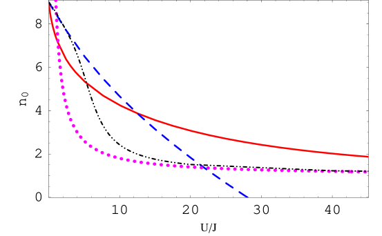
Figure 1: The occupation number for the homogeneous mode, as a function of $U$; $n=1$, $N_{s}=9$ and $J=1$. The solid-red line is our prediction, the black dash-dotted line is the exact numerical solution. The pink dots correspond to first order strong coupling perturbation theory, and the blue-dashed line to the PNC method.

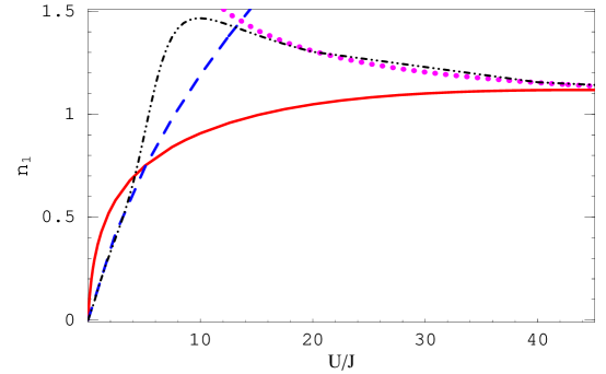
Figure 2: The occupation number for the first mode as a function of $U$; the conventions are the same as in Fig. 1.

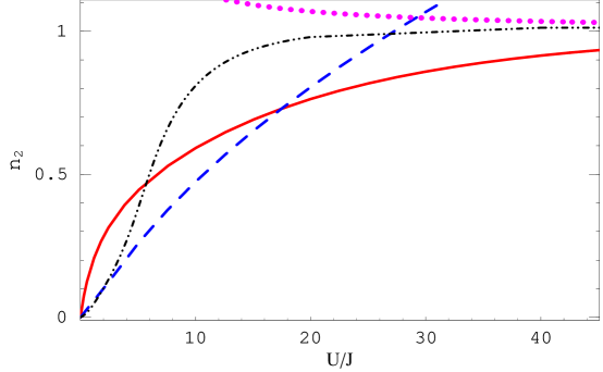
Figure 3: The occupation number for the second mode as a function of $U$; the conventions are the same as in Fig. 1.

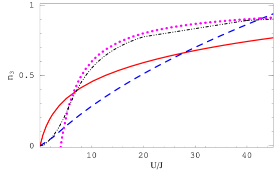
Figure 4: The occupation number for the third mode as a function of $U$; the conventions are the same as in Fig. 1.

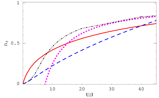
Figure 5: The occupation number for the fourth mode as a function of $U$; the conventions are the same as in Fig. 1.

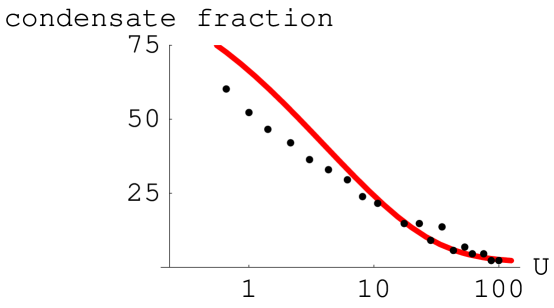
Figure 6: Condensate fraction ($\%$) plotted against $U$. Red solid line: prediction from our model using the parameters $n=1$, $N_{s}=61$ and $J=1$, Dots: Experimental points obtained from Fig. 4a in Ref SMSKE04 .

VII.2 Remarks

In this paper we have presented an analytic approximation for the one body density matrix (or equivalently, its Fourier transform, the momentum distribution) for a cold gas of structureless bosons in an homogeneous optical lattice. We have focused on the regime of low integer filling factor near the superfluid - insulator transition, which is not sufficiently covered in the literature. We have checked our results against exact calculations for small lattices, and against the theoretical predictions from the Bogoliubov approach and first order strong coupling perturbation theory. Our model interpolates between these theoretical alternatives, keeping an uniform accuracy in the transition region.

Our model works deep in the MI region, because it is built to be exact when $J=0$. This is an advantage of our choice of variables over the usual density -phase variables. In the superfluid regime the model predicts that quantum fluctuations in the $X_{p}$ degrees of freedom scale like $U$ (cf. Eq. (133) and thus also qualitatively captures the decay of condensate population and the increase of non-condensate atoms.

However, the agreement is not perfect. The qualitative but not quantitative agreement suggest that higher order corrections are required for a proper description of the physics. For observables like the number fluctuations at one site, which vanish in the Mott regime according to the linearized approximation, for example, higher order corrections would be dominant.

Quantum corrections will also be important for the dynamic structure factor. There is no contradiction between the phonon spectrum of our model (cfr. Eq. (104)) and a gapped dynamic structure factor, because in the Mott regime the amplitudes of the single phonon poles go to zero, while other poles arise because of higher order corrections. However, in this paper, we have not presented actual results for the particle number fluctuations nor the dynamic structure factor; these must be included in the list of unfinished business we discussed in the introduction.

A preliminary comparison we made against available experimental results SMSKE04 ; SSMKE04 of the condensate fraction from an array of one-dimensional lattices contained within a three dimensional trap for variable $U/J$ showed fair agreement between the experimental results and the predictions of our model. In these experiments, the central tubes had around $N_{s}=60$ populated sites SSMKE04 . The mean occupation number was close to $n=2$ near the center of the trap, and close to $n=1$ if averaged over all lattices K05 . We have compared the experimental results to the predictions of our model for several values of $N_{s}$ around $60,$ and filling fractions $n=1$ and $2.$ The results are fairly independent of $N_{s}$ in this range, and very sensitive to $n$ instead. As a typical representative, we show in Fig. 6 the prediction of our model for the condensate fraction for $N_{s}=61$ and $n=1.$We have superimposed the experimental results as reported in SMSKE04 .

We do not regard this as a validation of our model, since it was derived for a translationally invariant lattice and the parabolic confinement is not adequately included in our model. Nevertheless, the agreement is encouraging and suggest that our model might be more suitable for trapped systems as in this case, in contrast to the commensurate translationally invariant lattice, there is not a sharp MI transition. We defer a detailed discussion to a future communication RHC05 .

In summary, in our view, the most important contribution of this work is that it is the first step in the formulation of a quantum field theoretical approach capable of dealing with the intermediate regime. Even though the agreement with exact numerical solutions is not perfect, we find it satisfactory because we are using only the first order approximation. It is a reasonable expectation that by including higher order corrections we might narrow the present gap. We are perhaps still a long way from a reliable, fully nonequilibrium model of the initialization process of a QIP device based on cold atoms on an optical lattice, but from this work we have gained some confidence that we are moving in the right direction.

Acknowledgments EC acknowledges support from Universidad de Buenos Aires, CONICET and ANPCyT (Argentina); BLH from NSF grant PHY-0426696.

A.M. Rey is supported from an the Advanced Research and Development Activity (ARDA) contract and the U.S. National Science Foundation through a grant PHY-0100767 and a grant from the Institute of Theoretical, Atomic, Molecular and Optical Physics at Harvard University and Smithsonian Astrophysical observatory.

We thank M. Köhl for pointing out the relevance of refs. SMSKE04 ; SSMKE04 to this work and for discussing details of the experiment with us, and V. Penna, M. Martin-Delgado and M. Rigol for useful comments.

Appendix A Approximate approaches to the momentum distribution function

In this appendix we shall derive the formulae we plotted in the Figures to match against our model. We include it only to dispell any ambiguity regarding notation.

A.1 Strong coupling Rayleigh - Schrodinger perturbation theory

This is just ordinary perturbation theory in the parameter $J,$ starting from the state $\left|MI\right\rangle$ in Eq. (7). The BH Hamiltonian Eq. (1) is written as $H=H_{0}+H_{1},$ where $H_{0}$ is the $U$ term and $H_{1}=-\sum_{ij}J_{ij}a_{i}^{\dagger}a_{j}.$ Since $\left\langle MI\left|H_{1}\right|MI\right\rangle=0$, the vacuum energy is unchanged to first order. $H_{1}\left|MI\right\rangle$ is a superposition of one particle-hole states, all of which have energy $U$ above the vacuum, so the first order ground state is

$$\left|T\right\rangle=\left|MI\right\rangle-\frac{1}{U}H_{1}\left|MI\right\rangle$$ (147)

and the momentum distribution function is

$$n_{q}=n+\frac{4J}{U}n\left(n+1\right)\cos\left[2\pi\frac{q}{N_{s}}\right]$$ (148)

A.2 The PNC method

To simplify the problem, we shall consider only the case of a homogeneous, time - independent lattice.

The starting point of the method is the Heisenberg equation of motion for the destruction operator $a_{j}$

$$\left(-i\right)\frac{\partial}{\partial t}a_{j}\left(t\right)=\left[H,a_{j}\left(t\right)\right]=\sum_{i}J_{ij}a_{i}-Ua_{j}^{\dagger}a_{j}^{2},$$ (149)

Parameterize

$$a_{j}=\frac{e^{-i\mu t}}{\sqrt{N_{s}}}a_{0}\left[1+\sum_{p\neq 0}e^{2\pi ipj/N_{s}}\Lambda_{p}\right]$$ (150)

There are three key observations: 1) the operators $\Lambda_{p}$ preserve total particle number, 2) the fact that the one-body density matrix allows for a homogeneous eigenvector implies $\left\langle a_{0}^{\dagger}a_{0}\Lambda_{p}\right\rangle=0$ for all $p$, and 3) we have the exact identity

$$a_{0}^{\dagger}a_{0}\left[1+\sum_{p\neq 0}\Lambda_{p}^{\dagger}\Lambda_{p}\right]=N$$ (151)

Now we develop a perturbative expansion in inverse powers of $N,$ assuming $a_{0}\sim O\left(\sqrt{N}\right)$ and $\Lambda_{p}\sim O\left(1/\sqrt{N}\right).$ Multiplying Eq. (149) by $a_{0}^{\dagger}$ we get, to first order

$$\mu=Un-2J$$ (152)

$$i\frac{d\Lambda_{p}}{dt}=\frac{\nu_{p}}{2}\Lambda_{p}+Un\left(\Lambda_{p}+\Lambda_{-p}^{\dagger}\right)$$ (153)

As usual, we seek a solution through a Bogoliubov transformation. Taking into account the commutation relations for the $\Lambda_{p}$ we get

$$\Lambda_{p}=\frac{1}{\sqrt{N}}\left\{e^{-i\omega_{p}t}c_{p}A_{p}+e^{i\omega_{p}t}s_{p}A_{-p}^{\dagger}\right\}$$ (154)

$$c_{p}^{2}-s_{p}^{2}=1$$ (155)

(in this simple problem, we may assume the Bogoliubov coefficients are real). We get

$$\left[\omega_{p}-Un-\frac{\nu_{p}}{2}\right]c_{p}-Uns_{p}=0$$ (156)

$$Unc_{p}+\left[\omega_{p}+Un+\frac{\nu_{p}}{2}\right]s_{p}=0$$ (157)

from where we recover the dispersion relation Eq. (104) and

$$s_{p}=-\frac{1}{\sqrt{2}}\left[\frac{Un+\frac{\nu_{p}}{2}}{\omega_{p}}-1\right]^{1/2}$$ (158)

The momentum distribution function is $n_{p}=s_{p}^{2}$ for $p\neq 0$, and $n_{0}=N-\sum_{p\neq 0}n_{p}$ for the homogeneous mode.

Appendix B Approximate formula for the one-body density matrix

The idea is to evaluate Eq. (140) by decomposing the quadratic term in a sum of squares. Of course, one possibility is to write

$$k_{j}=\frac{1}{\sqrt{N_{s}}}\sum_{p}e^{2\pi ipj/N_{s}}\widetilde{k}_{p}$$ (159)

The problem is that the requirement that all $k_{j}$ be integer places a highly nontrivial constraint on the $\widetilde{k}_{p}.$

Consider instead the functions

$$f_{p}\left(j\right)=\mathrm{sign}\left[\cos\left[\frac{2\pi pj}{N_{s}}\right]\right]$$ (160)

$$g_{p}\left(j\right)=\mathrm{sign}\left[\sin\left[\frac{2\pi pj}{N_{s}}\right]\right]$$ (161)

These functions are not orthogonal, but they are a basis. Therefore we can always write

$$k_{j}=a_{0}+\frac{1}{2}\sum_{p>0}\left(a_{p}f_{p}\left(j\right)+b_{p}g_{p}\left(j\right)\right)$$ (162)

Observe that $f_{0}$ is always a null eigenvector of $M_{ij}.$ We expect the $f$ and $g^{\prime}$s will be approximate eigenvectors. For a large number of sites, $e^{2\pi iqj/N_{s}}$ and $f_{p},g_{p}$ will be nearly orthogonal unless $q=\pm p,$ and we shall have

$$f_{p}\left(j\right)\sim\frac{2}{N_{s}}\left\{1+2\sum_{l>0}\left|\cos\left[\frac{2\pi pl}{N_{s}}\right]\right|\right\}\cos\left[\frac{2\pi pj}{N_{s}}\right]$$ (163)

$$g_{p}\left(j\right)\sim\frac{4}{N_{s}}\left\{\sum_{l>0}\left|\sin\left[\frac{2\pi pl}{N_{s}}\right]\right|\right\}\sin\left[\frac{2\pi pj}{N_{s}}\right]$$ (164)

So

$$\sum_{l}M_{jl}f_{p}\left(l\right)\sim A_{p}f_{p}\left(j\right)$$ (165)

$$\sum_{l}M_{jl}g_{p}\left(l\right)\sim A_{p}g_{p}\left(j\right)$$ (166)

where of course $A_{0}=0$ and

$$A_{p}=\frac{n\nu_{p}}{2\omega_{p}}\qquad p\neq 0$$ (167)

Then from the decomposition Eq. (162) we get

$$\sum_{i}k_{i}v_{i}^{m}=\sum_{p>0}\left(a_{p}C_{p}^{m}-b_{p}D_{p}^{m}\right)$$ (168)

$$\sum_{ij}k_{i}M_{ij}k_{j}=\sum_{p>0}\left(a_{p}^{2}E_{p}+b_{p}^{2}F_{p}\right)$$ (169)

where the coefficients are given in Eqs. (143), (144), (145) and (146).

Although each term of the series Eq. (140) factorizes, there are correlations among the $a$  and $b$ coefficients from the discreteness of the $k_{j}.$ For example, for three sites we have that $b_{1}=k_{1}-k_{-1}$ must be an integer, but $a_{1}=k_{0}-k_{1}+(b_{1}/2)$ will be integer if $b_{1}$ is even or half-integer if $b_{1}$ is odd. However, when the number of sites is large we may neglect these correlations, and assume that the $a$ and $b$ coefficients simply take integer values. Under this approximation, the multiple sum Eq. (140) factorizes, and we obtain Eq. (142), where $\vartheta_{3}$ is the Elliptic Theta function WW02

$$\vartheta_{3}\left(z,q\right)=1+2\sum_{n=1}^{\infty}q^{n^{2}}\cos\left[2nz\right]$$ (170)

References

- (1) E. A. Cornell and C. E. Wieman, Nobel Lecture: Bose-Einstein condensation in a dilute gas, the first 70 years and some recent experiments , Rev. Mod. Phys. 74, 875-893 (2002); W. Ketterle, Nobel lecture: When atoms behave as waves: Bose-Einstein condensation and the atom laser , Rev. Mod. Phys. 74, 1131-1151 (2002).
- (2) K. Southwell (editor), Nature Insight: Ultracold matter, Nature 416, 205 (2002).
- (3) D. Jaksch and P. Zoller, The cold atom Hubbard toolbox, cond-mat/0410614.
- (4) O. Mandel et al., Controlled collisions for multiparticle entanglement of optically trapped atoms, Nature 425, 937 (2003).
- (5) See D. Vager, B. Segev and Y. Band, Engineering entanglement: the fast-approach phase gate, quant-ph/0505199 and references therein.
- (6) G. Brennen et al, Quantum computer architecture using non-local interactions, Phys. Rev. A67, 050302 (2003).
- (7) G. K. Brennen et al., Scalable register initialization for quantum computing in an optical lattice, quant-ph/0312069; G. Pupillo et al., Scalable quantum computation in systems with Bose-Hubbard dynamics, J. Mod. Opt. 51, 16 (2004); A. M. Rey, P. B. Blakie and C. W. Clark, Dynamics of a period 3 pattern-loaded BEC in an optical lattice, Phys. Rev. A67, 053610 (2003).
- (8) J. Dziarmaga, A. Smerzi, W. Zurek and A. Bishop Non-equilibrium Mott transition in a lattice of Bose-Einstein condensates cond-mat/0403607 Proceedings of NATO ASI Patterns of symmetry breaking, Krakow, Poland, Sept. 2002.
- (9) S. Tsuchiya and A. Griffin, Landau damping of Bogoliubov excitations in optical lattices at finite temperature, cond-mat/0506016.
- (10) M. Fisher, P. Weichman, G. Grinstein and D. Fisher Boson localization and the superfluid-insulator transition Phys. Rev. B 40, 546 (89)
- (11) Greiner et al Nature 415, 39 (02).
- (12) O. Penrose and L. Onsager Bose-Einstein condensation and liquid helium Phys. Rev. 104, 576 (1956).
- (13) F. Gerbier et al., Phase coherence of an atomic Mott insulator, cond-mat/0503452.
- (14) F. Gerbier et al., Interference pattern and visibility of a Mott insulator, cond-mat/0507087
- (15) R. Roth and K. Burnett, Superfluidity and interference pattern of ultracold bosons in optical lattices, Phys. Rev. A 67, 031602 (R) (2003); Y. Yu, Short-range coherence in a Bose atom Mott insulator, cond-mat/0505181.
- (16) A. M. Rey, K. Burnett, R. Roth, M. Edwards, C. Williams and C. Clark, Bogoliubov approach to superfluidity of atoms in an optical lattice, J. Phys. B36, 825 (2003).
- (17) J. Freericks and H. Monien Phase diagram of the Bose Hubbard model Europhys. Lett. 26, 545 (1994).
- (18) J. Freericks and H. Monien Strong-coupling expansion for the pure and disordered Bose-Hubbard model Phys. Rev. B 53, 2691 (1996).
- (19) N. Elstner and H. Monien, Dynamics and thermodynamics of the Bose-Hubbard model Phys. Rev. B 59, 12184 (1999)
- (20) A. M. Rey, P. Blair Blackie, G. Pupillo, C. Williams and C. Clark, Bragg spectroscopy of ultracold atoms loaded in an optical lattice, cond-mat/0406552.
- (21) P. Blair Blakie and C. Clark, Wannier states and Bose-Hubbard parameters for 2D optical lattices, cond-mat/0403306.
- (22) G. Batrouni, R. Scalettar and G. Zimanyi Quantum critical phenomena in one-dimensional Bose systems Phys. Rev. Lett 65, 1765 (1990); G. Batrouni and R. Scalettar World-line quantum Monte Carlo algorithm for a one-dimensional Bose model Phys. Rev. B46, 9051 (1992)
- (23) S. Clark and D. Jaksch Dynamics of the superfluid to Mott insulator transition in one dimension Phys. Rev. A70, 043612 (2004).
- (24) A. Kampf and G. Zimanyi, Superconductor-insulator phase transition in the boson Hubbard model Phys. Rev. B 47, 279 (1993); K. Sheshadri et al., Superfluid and insulating phases in an interacting-boson model: mean field theory and the RPA, Europhys. Lett. 22, 257 (1993); D. Jaksch, C. Bruder, J. Cirac, C. Gardiner and P. Zoller Cold bosonic atoms in optical lattices Phys. Rev. Lett 81, 3108 (1998); L. Amico and V. Penna Dynamical mean field theory of the Bose-Hubbard model Phys. Rev. Lett. 80, 2189 (1998); D. van Oosten, P. van der Straten and H. Stoof Quantum phases in an optical lattice Phys. Rev. A 63, 53601 (2001); D. van Oosten, P. van der Straten and H. Stoof Mott insulators in an optical lattice with large filling factors, Phys. Rev. A67, 033606 (2003); A. Polkovnikov, S. Sachdev and S. Girvin Nonequilibrium Gross-Pitaevskii dynamics of boson lattice models Phys. Rev. A 66, 53607 (2002); W. Zwerger, Mott-Hubbard transition of cold atoms in optical lattices, J. Opt. B: Quantum Semiclass. Opt. 5, S9 (2003); P. Buonsante, R. Franziosi and V. Penna From the superfluid to the Mott regime and back: triggering a non-trivial dynamics in an array of coupled condensates J. Phys. B37, S195 (2004); P. Buonsante, V. Penna and A. Vezzani Analytical mean-field approach to the phase-diagram of ultracold bosons in optical superlattices Laser Physics 15 (2), 361 (2005); I. Carusotto and Y. Castin, An exact reformulation of the Bose-Hubbard Model in terms of a stochastic Gutzwiller ansatz, cond-mat/0303259; J. Zakrzewski, On quantum phase transition in a gas of ultracold atoms, cond-mat/0406186.
- (25) C. Schroll, F. Marquardt and C. Bruder, Perturbative corrections to the mean field solution of the Mott - Hubbard model, Phys. Rev. A70, 053609 (2004).
- (26) P. Buonsante and A. Vezzani, Second order cell strong coupling perturbative expansion for superlattice Bose-Hubbard models, cond-mat/0503232.
- (27) M. Kramer, L. Pitaievskii and S. Stringari, Macroscopic dynamics of a trapped BEC in the presence of 1D and 2D optical lattices, Phys. Rev. Lett. 88, 180404 (2002).
- (28) M. Girardeau and R. Arnowitt Theory of many-boson systems: pair theory Phys. Rev. 113, 755 (1959); Y. Castin and R. Dum Instability and depletion of an excited Bose-Einstein condensate in a trap Phys. Rev. Lett. 79, 3553 (1997); Y. Castin and R. Dum Low-temperature Bose-Einstein condensates in time-dependent traps: Beyond the U(1) symmetry breaking approach Phys. Rev. A57, 3008 (1998); C. Gardiner Particle-number-conserving Bogoliubov method which demonstrates the validity of the time-dependent Gross-Pitaevskii equation for a highly condensed Bose gas Phys. Rev. A56, 1414 (1997); S. Gardiner, D. Jaksch, R. Dum, J. Cirac and P. Zoller Nonlinear matter wave dynamics with a chaotic potential Phys. Rev. A62, 23612 (2000); S. Morgan The response of Bose-Einstein condensates to external perturbations at finite temperature Phys. Rev. A69, 023609 (2004); Z. Idziaszek Microcanonical fluctuations of the condensate in a weakly interacting Bose gas Phys. Rev. A71, 053604 (2005); J. Dziarmaga, Images of a Bose-Einstein condensate at finite temperature, cond-mat/0506723.
- (29) See J. Andersen, Theory of the weakly interacting Bose gas Rev. Mod. Phys. 76, 599 (2004) and references therein.
- (30) Ana Maria Rey, B. L. Hu, Esteban Calzetta, Albert Roura, Charles Clark, Nonequilibrium Dynamics of Optical Lattice-Loaded BEC Atoms: Beyond HFB approximation, Phys. Rev. A 69, 033610 (2004) [cond-mat/0308305]; Ana Maria Rey, B. L. Hu, Esteban Calzetta and Charles Clark, “Quantum kinetic theory of a Bose-Einstein gas confined in a lattice ”, Phys. Rev. A (to appear); K. Goral, T. Köhler, T. Gasenzer and K. Burnett, Dynamics of correlations in atomic Bose-Einstein condensates, J. Mod. Opt. 51, 1731 (2004).
- (31) J-J. Liang, J-Q. Liang and W. Liu Quantum phase transition of condensed bosons in optical lattices Phys. Rev. A68, 43605 (2003).
- (32) K. Sengupta and N. Dupuis, Mott insulator to superfluid transition in the Bose-Hubbard model: a strong coupling approach, Phys. Rev. A71, 033629 (2005); Mott insulator to superfluid transition of ultracold bosons in an optical lattice near a Feshbach resonance, cond-mat/0406396.
- (33) B. Paredes et al. Tonks-Girardeau gas of ultracold atoms in an optical lattice Nature 429, 277 (2004); M. Holland Atomic beads on strings of light Nature 429, 251 (2004); M. Girardeau, J. Math. Phys. 1, 516(1960) E. H. Lieb and W. Liniger, Phys. Rev. 130, 1605 (1963). T. Kinoshita, T. Wenger and D. S. Weiss, Science 305, 1125 (2004). M. A. Cazalilla,Physical Review A 67, 053606 (2003). M. A. Cazalilla, Phys. Rev. A 70, 041604(R) (2004); L. Salasnich, A. Parola and L. Reatto, Quasi one-dimensional bosons in three-dimensional traps: from strong coupling to weak coupling regimes, cond-mat/0507190.
- (34) G. Pupillo, A. Rey, C. Williams and C. Clark, Pseudofermionization of 1-d bosons in optical lattices, cond-mat/0505325.
- (35) R. Fresard Slave boson formulation for interacting boson systems and the superfluid-insulator transition cond-mat/9405053; D. Dickerscheid, D. van Oosten, P. Denteneer and H. Stoof Ultracold atoms in optical lattices Phys. Rev. A68, 43623 (2003); Y. Yu, S. Chui, Phase diagram of ultracold atoms on optical lattice: comparative study to slave fermion and slave boson for Bose Hubbard model, Phys. Rev. A71, 033608 (2005).
- (36) E. Madelung, Quantentheorie in hydrodynamischer Form, Zeitschrift fur physik XL, 322 (1927)
- (37) F. Haldane, Effective harmonic-fluid approach to low-energy properties of one-dimensional quantum fluids, Phys. Rev. Lett. 47, 1840 (1981)
- (38) P. Carruthers and M. Nieto Phase and angle variables in quantum mechanics Rev. Mod. Phys. 40, 411 (1968); D. Pegg and S. Barnett Phase properties of the quantized single-mode electromagnetic field Phys. Rev. A39, 1665 (1989); J. Vargas-Martinez and H. Moya-Cessa On the quantum phase problem J. Opt. B6, S155 (2004).
- (39) L. Amico and V. Penna Time-dependent mean field theory of the superfluid-insulator phase transition Phys. Rev. B62, 1224 (2000); J. Anglin, P. Drummond and A. Smerzi Exact quantum phase model for mesoscopic Josephson junctions Phys. Rev. A64, 63605 (2001); C. Mora and Y. Castin Extension of Bogoliubov theory to quasicondensates Phys. Rev. A67, 53615 (2003); Y. Castin Simple theoretical tools for low dimension Bose gases cond-mat/0407118; Z. Nazario and D. Santiago On the existence of roton excitations in Bose-Einstein condensates: signature of proximity to a Mott insulating phase cond-mat/0403408; L. Balents, L. Bartosch, A. Burkov, S. Sachdev and K. Sengupta Putting competing orders in their place near the Mott transition Phys. Rev. B71, 144508 (2005); L. Balents et al., Competing orders and non - Landau - Ginzburg - Wilson criticality in (Bose) Mott transitions, cond-mat/0504692.
- (40) S. Sachdev, Quantum Phase Transitions (Cambridge University Press, Cambridge, England, 1999).
- (41) A. Polkovnikov et al., Decay of super-currents in condensates in optical lattices, cond-mat/0504300.
- (42) H. Buchler, G. Blatter and W. Zwerger, Commensurate- Incommensurate transition of cold atoms in an optical lattice, PRL90, 130401 (2003).
- (43) E. Altman and A. Auerbach Oscillating superfluidity of bosons in optical lattices Phys. Rev. Lett. 89, 250404 (2002); S. Sachdev, K. Sengupta and S. Girvin Mott insulators in strong electric fields Phys. Rev. B66, 75128 (2002); K. Sengupta, S. Powell and S. Sachdev Quench dynamics across quantum critical points cond-mat/0311355; M. Aizenman, E. Lieb, R. Seiringer, J. Solovej and J. Yngvason Bose-Einstein condensation as a quantum phase transition in an optical lattice cond-mat/0412034; A. Polkovnikov, E. Altman, E. Demler, B. Halperin and M. Lukin Decay of a superfluid current in a moving system of strongly interacting bosons Phys. Rev. A71, 063613 (2005).
- (44) A. K. Tuchman et al. Nonequilibrium coherence dynamics of a soft boson lattice, cond-mat/0504762; A. Polkovnikov, Evolution of the macroscopically entangles states in optical lattices, Phys. Rev. A68, 033609 (2003), Quantum corrections to the dynamics of interacting bosons: beyond the Truncated Wigner Approximation, Phys. Rev. A68, 053604 (2003); L. Isella and J. Ruostekoski, Nonadiabatic dynamics of a BEC in an optical lattice, cond-mat/0409475.
- (45) P. Jain and C. Gardiner, A phase space method for the Bose-Hubbard Model, cond-mat/0404642.
- (46) J. S. Schwinger,J. Math. Phys,2 407(1961) L. V. Keldysh, Zh. Eksp. Teor. Fiz. 47 , 1515 (1964) [Engl. trans. Sov. JETP 20 1018 (1965)]. V. Korenman, Ann. Phys,39 72 (1966). G. Zhou, Z. Su, B. Hao and L. Yu, Phys. Rep. 118, 1 (1985).
- (47) J. Andersen, U. Al Khawaja and H. T. C. Stoof, Phase fluctuations in atomic Bose gases, Phys. Rev. Lett. 88, 070407 (2002); N. Proukakis, Density fluctuations in ultracold one-dimensional Bose gases, cond-mat/0505039.
- (48) S. Friebel et al., CO2 laser optical lattice with cold rubidium atoms, Phys. Rev. A57, R20 (1998).
- (49) E. Calzetta and B-L. Hu, Gauge-invariant Effective Action for the Dynamics of Bose-Einstein condensates with a fixed number of atoms, cond-mat/0508240.
- (50) P. Lee and N. Nagaosa, Gauge theory of the normal state of high- superconductors, Phys. Rev. B46, 5621 (1992).
- (51) P. Dirac, Generalized Hamiltonian Dynamics, Can. J. Math. 2, 129 (1950); Proc. R. Soc. London A246, 326 (1958); Lectures on Quantum Field Theory, Yeshiva University, New York, 1965.
- (52) M. Peskin and D. Schroeder, An introduction to Quantum Field Theory (Addison Wesley, NY (1995)).
- (53) C. Orzel et al., Squeezed states in a Bose Einstein Condensate, Science 291, 2386 (2001).
- (54) M. Köhl et al., Superfluid to Mott insulator transition in one, two and three dimensions, J. Low. T. Phys 138, 635 (2005).
- (55) A. M. Rey, G. Pupillo, C. Clark and C. Williams, Ultracold atoms confined in an optical lattice plus a parabolic potential: a closed-form approach, cond-mat/0503477; E. Mariani and A. Stern, Localized excitations at the Mott insulator - superfluid interfaces for confined BECs, cond-mat/0505755.
- (56) G. Batrouni et al., Dynamic response of trapped ultracold bosons on optical lattices, cond-mat/0503371; V. Kashurnikov, N. Prokof’ev and B. Svistunov, Revealing the superfluid - Mott insulator transition in an optical lattice, Phys. Rev. A66, 031601 (2002); J. Zakrewski, Mean field dynamics of the superfluid-insulator phase transition in a gas of ultra cold atoms, Phys. Rev. A71, 043601 (2005); S. Wessel et al., Quantum Monte Carlo simulations of confined bosonic atoms in optical lattices, Phys. Rev. A70, 053615 (2004); B. de Marco et al., Structure and stability of Mott insulator shells of bosons trapped in an optical lattice, cond-mat/0501718.
- (57) T. Savard, K. O’Hara and J. Thomas, Laser - noise - induced heating in far - off resonance optical traps, Phys. Rev. A56, R1095 (1997).
- (58) D. van Oosten, P. van der Straten and H. T. C. Stoof, Thermal fluctuations and the superfluid to Mott insulator transition, cond-mat/0205066; G. Pupillo, C. Williams and N. Prokof’ev, Accurate and robust temperature measurement for ultracold atoms in deep optical lattices, cond-mat/0407075; A. Reischl, K. Schmidt and G. Uhrig, Temperature in one-dimensional bosonic Mott insulators, cond-mat/0504724.
- (59) E. Altman, W. Hofstetter, E. Demler and M. Lukin, Phase diagram of two-component bosons on an optical lattice, New J. of Phys. 5, 113.1 (2003).
- (60) T. Stoferle et al., Transition from a strongly interacting 1D superfluid to a Mott insulator, Phys. Rev. Lett. 92, 130403 (2004).
- (61) C. Schori et al., Excitations of a superfluid in a 3D optical lattice, Phys. Rev. Lett. 93, 240402 (2004).
- (62) A. M. Rey, B-L. Hu and E. Calzetta, in preparation.
- (63) J. Negele and H. Orland, Quantum many-particle systems (Perseus Books, New York, 1998).
- (64) S. Coleman, Aspects of Symmetry (Cambridge University Press, Cambridge, England, 1985).
- (65) E. Calzetta and B-L. Hu, Phys. Rev. D35, 495 (1987).
- (66) E. Calzetta and B-L. Hu, Phys. Rev. D37, 2878 (1988).
- (67) H. Kleinert, Path Integrals in quantum mechanics, statistics and polimer physics (World Scientific, Singapore, 1990).
- (68) P. Drummond, P. Deuar and K. Kheruntsyan, Canonical Bose gas simulations with stochastic gauges, Phys. Rev. Lett 92, 040405 (2004).
- (69) E. T. Whittaker and G. N. Watson, A Course of Modern Analysis (Cambridge University Press, Cambridge (England), 1984).
- (70) M. Köhl, private communication.