Generalized band anti-crossing model for highly mismatched semiconductors applied to BeSe_xTe_1-x

Abstract

We report a new model for highly mismatched semiconductor (HMS) alloys. Based on the Anderson impurity Hamiltonian, the model generalizes the recent band anti-crossing (BAC) model, which successfully explains the band bowing in highly mismatched semiconductors. Our model is formulated in empirical tight-binding (ETB) theory and uses the so called sp³s* parameterization. It does not need extra parameters other than bulk ones. The model has been applied to BeSe_xTe_1-x alloy. BeTe and BeSe are wide-band gap and highly mismatched semiconductors. Calculations show large band bowing, larger on the Se rich side than on the Te rich side. Linear interpolation is used for an arbitrary concentration $x$. The results are applied to calculation of electronic and optical properties of BeSe_0.41Te_0.59 lattice matched to Si in a superlattice configuration.

I Introduction

In recent years there has been a tremendous interest in electro-optical properties of II-VI semiconductors in particular epitaxial II-VI heterostructures. New developments Clark et al. (2000); Kirk et al. (2000) in the growth of Si lattice-matched BeSe_0.41Te_0.59 open the opportunity to a new class of Si based devices. Be-chalcogenides are wide-band gap zinc blende semiconductors with lattice constants close to that of Si. Thus BeTe and BeSe have the lattice constants of 5.6269 and 5.1477 Å, respectively, 3.6 % larger and 5.2 % smaller than Si. Vegard’s law says that the lattice matched composition with Si is BeSe_0.41Te_0.59. Therefore Be-chalcogenides are candidates for Si-based heterostructures.

The difference in size and orbital energies between Se and Te in addition to large lattice mismatch between BeTe and BeSe makes the virtual-crystal approximation (VCA) inappropriate for the ternary alloy BeSe_xTe_1-x. The band anti-crossing (BAC) model Walukiewicz et al. (2000) has been introduced in order to explain the electronic structure of highly mismatched III-V-N alloys and II-VI alloys like ZnSe_xTe_1-x Wu and et al. (2003a). At impurity like concentrations close to both end points, the electronegativity difference between constituent elements gives rise to localized energy levels close to the conduction or valence band. Thus in the ZnSe(ZnTe)-rich side, the band gap bowing is mostly determined by the anticrossing interaction between the Te(Se) localized level, which behaves like an impurity, and the extended states of ZnSe valence band (ZnTe conduction band) near the center of the Brillouin zone Wu and et al. (2003b).

In this communication we develop a model which is a natural extension of the BAC model to empirical tight-binding (ETB). Based on this model we determine optical bandgap of BeSe_xTe_1-x alloy and further we analyze the band folding in Si/BeSe_0.41Te_0.59 heterostructures.

II Model

There are several studies employing tight-binding (TB) models for HMS. They use either supercells O’Reilly et al. (2002) or add extra parameters to the usual TB parameters within the BAC model Shtinkov et al. (2003). Our approach needs no extra parameters others than the usual TB parameters and is a natural extension of the BAC model to TB. We consider first the dilute limit. The starting point is the impurity model of Anderson Anderson (1961). Consider a complex-structured impurity interacting with the host crystal having the Hamiltonian

$$H=H_{c}+H_{imp}+V=H_{0}+V$$ (1)

where $H_{c}$ is Hamiltonian of the host crystal, $H_{imp}$ is the Hamiltonian of the impurity and $V$ is the Hamiltonian of the interaction between impurity and crystal. The above Hamiltonians have the following expressions

$$H_{imp}=\sum\limits_{p,d,\sigma}{\varepsilon_{d\sigma}c_{pd\sigma}^{+}c_{pd\sigma}},$$ (2)

$$H_{c}=\sum\limits_{i,k,\sigma}{\varepsilon_{ik\sigma}c_{ik\sigma}^{+}c_{ik\sigma}},$$ (3)

$$V=\sum\limits_{p,d,i,k,\sigma}{\left({V_{ikd}c_{pd\sigma}^{+}c_{ik\sigma}+h.c.}\right)}.$$ (4)

Here $\sigma$ is the spin index, $d$ are the energy levels of impurity at the $p$th site ($N_{i}$, the total number of impurities), $i$ is band index of the crystal, $k$ is the wavevector, $c_{pd\sigma}^{+}(c_{pd\sigma})$are the creation (annihilation) operators of electrons on impurity levels. $c_{ik\sigma}^{+}(c_{ik\sigma})$ are the creation (annihilation) operators of electrons of the bands in the crystal, and $V$ is the coupling between impurity and crystal and has factor $1\mathord{\left/{\vphantom{1{\sqrt{N}}}}\right.\kern-1.2pt}{\sqrt{N}}$ with $N$ total number of sites. In order to calculate the effect of impurity we shall use an expression for the projection of $H$ into ${\rm H}$, a subspace of the Hilbert space spanned by the Hamiltonian $H_{0}$. We define $P$ (and $Q)$ the projections onto (out of) ${\rm H}$ as $P^{2}=P$, $Q^{2}=Q$, $P+Q=1$, $PQ=0$, $\left[{P,H_{0}}\right]=\left[{Q,H_{0}}\right]=0$. Let the Green function of the entire system be denoted by $G\left(z\right)=\left({z-H}\right)^{-1}$ and the projected part onto ${\rm H}$ as $\overline{G}\left(z\right)=PG\left(z\right)P$. In this way we denote the projection onto ${\rm H}$ of any operator $A$ as: $\overline{A}=PAP$. Straightforward algebra gives us

$$\overline{G}\left(z\right)=\frac{1}{z-\overline{H}_{0}-\overline{R}\left(z\right)},$$ (5)

where $\overline{R}\left(z\right)=PVP+PV\frac{Q}{z-H_{0}-QVQ}VP$. One can expand $\overline{R}\left(z\right)$ for small $V$

$$\overline{R}\left(z\right)=PVP+PV\frac{Q}{z-H_{0}}VP+PV\frac{Q}{z-H_{0}}V\frac{Q}{z-H_{0}}VP+\ldots.$$ (6)

Due to $Q$ in the expansion, all the intermediate states are outside of ${\rm H}$, therefore the diagrams representing $\overline{R}\left(z\right)$ must be irreducible. If $\overline{R}\left(z\right)$ is small compared to $H_{c}$, Eq. (5) can be expanded in a power series of $\overline{R}\left(z\right)$ as

$$\overline{G}\left(z\right)=G_{c}+G_{c}\overline{R}G_{c}+G_{c}\overline{R}G_{c}\overline{R}G_{c}+\ldots.$$ (7)

No approximations have been made so far. If $V$ is small we can replace $\overline{R}\left(z\right)$ in Eq. (6) by the first two terms and summing up all contributions (the first one is 0 in our model). By making such an approximation we, in fact, sum an entire class of diagrams. The impurity averaging is made by noticing that all macroscopically observables are self-averaging, i.e. they have asymptotically exact values in the thermodynamic limit Lifshits (1964). In other words the average of the product of such quantities is equal (within asymptotic accuracy) to the product of their averages. Therefore the impurity averaging in Eq. (5) is simply taken as averaging $\overline{R\left(z\right)}$ in Eq. (6). By keeping the first two terms in Eq. (6), the model is equivalent to the optical model laid out in Ref. Yonezawa, 1964: it only brings the shift to the energy levels of the unperturbed Hamiltonian and gives the following form for the diagonal part of the Green function of $i$th band

$$G_{kk\sigma\sigma}^{ii}\left(z\right)=\frac{1}{1-\varepsilon_{ik\sigma}-x\sum\limits_{d}{\frac{\left|{V_{ikd}}\right|^{2}}{z-\varepsilon_{d\sigma}}}},$$ (8)

where $x$ is the dilute concentration. For one band and 1-level impurity the result is identical to the BAC model Walukiewicz et al. (2000); Wu and et al. (2003a, b); Wu et al. (2002). This result can be easily expanded to include pair impurity interactions in addition to single impurity interactions Fahy and O’Reily (2004).

III Application to sp³s^∗ TB Hamiltonian and Numerical Results

The model laid out in the preceding section is directly applied to sp³s* Hamiltonian Vogl et al. (1983) with spin-orbit interaction Chadi (1977) The TB Hamiltonian is written in the sp³ hybrid basis and the basis is rotated in such a way that a unit cell is formed by the anion hybrid orbitals and the cation hybrid orbitals pointed toward the anion site. The s* orbitals remain unchanged. In the no spin-orbit case, the transformation is $H_{hyb}\left(k\right)=S^{+}\left(k\right)H_{AO}\left(k\right)S\left(k\right)$, where $H_{AO}\left(k\right)$ is the TB Hamiltonian in atomic (Lödwin) orbital basis and $H_{hyb}\left(k\right)$ the Hamiltonian in sp³ hybrid basis. The S matrix is block diagonal in anion/cation index and has the form for anion and cation site, respectively, as

$$\frac{1}{2}\left[{{\begin{array}[]{*{20}c}1\hfill&1\hfill&1\hfill&1\hfill&0\hfill\\ 1\hfill&1\hfill&{-1\hfill}&{-1\hfill}&0\hfill\\ 1\hfill&{-1\hfill}&1\hfill&{-1\hfill}&0\hfill\\ 1\hfill&{-1\hfill}&{-1\hfill}&1\hfill&0\hfill\\ 0\hfill&0\hfill&0\hfill&0\hfill&1\hfill\\ \end{array}}}\right],$$ (9)

$$\frac{1}{2}\left[{{\begin{array}[]{*{20}c}{e^{-ik\cdot{\kern 1.0pt}d_{1}}\hfill}&{e^{-ik\cdot{\kern 1.0pt}d_{2}}\hfill}&{e^{-ik\cdot{\kern 1.0pt}d_{3}}\hfill}&{e^{-ik\cdot{\kern 1.0pt}d_{4}}\hfill}&0\hfill\\ {-e^{-ik\cdot{\kern 1.0pt}d_{1}}\hfill}&{-e^{-ik\cdot{\kern 1.0pt}d_{2}}\hfill}&{e^{-ik\cdot{\kern 1.0pt}d_{3}}\hfill}&{e^{-ik\cdot{\kern 1.0pt}d_{4}}\hfill}&0\hfill\\ {-e^{-ik\cdot{\kern 1.0pt}d_{1}}\hfill}&{e^{-ik\cdot{\kern 1.0pt}d_{2}}\hfill}&{-e^{-ik\cdot{\kern 1.0pt}d_{3}}\hfill}&{e^{-ik\cdot{\kern 1.0pt}d_{4}}\hfill}&0\hfill\\ {-e^{-ik\cdot{\kern 1.0pt}d_{1}}\hfill}&{e^{-ik\cdot{\kern 1.0pt}d_{2}}\hfill}&{e^{-ik\cdot{\kern 1.0pt}d_{3}}\hfill}&{-e^{-ik\cdot{\kern 1.0pt}d_{4}}\hfill}&0\hfill\\ 0\hfill&0\hfill&0\hfill&0\hfill&1\hfill\\ \end{array}}}\right].$$ (10)

The vectors in (10) are ($a$ is the lattice constant): $d_{1}=\left({a\mathord{\left/{\vphantom{a4}}\right.\kern-1.2pt}4}\right)\left({1,1,1}\right)$,$d_{2}=\left({a\mathord{\left/{\vphantom{a4}}\right.\kern-1.2pt}4}\right)\left({1,\overline{1},\overline{1}}\right)$,$d_{3}=\left({a\mathord{\left/{\vphantom{a4}}\right.\kern-1.2pt}4}\right)\left({\overline{1},1,\overline{1}}\right)$, and $d_{4}=\left({a\mathord{\left/{\vphantom{a4}}\right.\kern-1.2pt}4}\right)\left({\overline{1},\overline{1},1}\right)$. An impurity is such a cell interacting through hybrid orbitals with the average/host crystal.

BeSe and BeTe are quite new materials. The nearest-neighbor sp³s* parameters were fitted to GW calculations Fleszar and Hanke (2000). They reproduce valence band edges $\Gamma_{8}$ and $\Gamma_{7}$, and the conduction band edges $\Gamma_{6}$ and $X_{1}$. The average crystal is considered by the average parameters. The hopping parameters were scaled according to the Harrison scaling rule Harrison (1989) and then averaged. The band offset between BeTe and BeSe is considered to be 0.41 eV as indicated in Ref.Bernardini et al., 2000. In this way one calculates the bowing of the on-site energies in addition to linear terms given by VCA. The hybrid states of the impurity lay outside bandgap of the host crystal, such that the net effect is large deviation from linearity of the band edges of the alloy. Mathematically one diagonalizes an extended Hamiltonian and accounts for the shifts in the band edges at the $\Gamma$ and X point in the Brillouin zone. Those shifts are used to calculate the bowing parameters for each self-energy.

We calculate the bowing parameters of the direct and indirect bandgap around 0 and 1 limits of concentration according to BAC model and follow the spirit of the VCA to interpolate linearly the effect of BAC model between these limits. The linear interpolation has been successfully used to fit experimental data for ZnSeTe alloy Wu and et al. (2003a, b). Linear interpolation for the direct and indirect bandgaps is consistent with linear interpolation performed on the tight-binding parameters. The tight-binding parameters for BeTe and BeSe are shown in Table 1. The bowing parameters of the on-site energies for Te-rich and Be-rich limit, respectively, are shown in parenthesis.

Table 1: Matrix elements in eV of nearest neighbor sp${}^{3}s^{*}$ model including spin-orbit interaction for BeTe and BeSe. The on-site energies of BeTe have been upgraded by 0.41 eV, the band offset between BeTe and BeSe. The notation is according to Vogl et al. Vogl et al. (1983). The bowing parameters of the on-site energies for BeTe-rich limit and BeSe-rich limit are shown in parenthesis. For a general concentration x the linear interpolation is used.

	BeTe	BeSe
E(s,c)	5.112+0.41 (-1.85)	5.560 (0.55)
E(s,a)	-15.401+0.41 (0.84)	-14.953 (1.0)
E(p,c)	4.427+0.41 (-0.6)	5.026 (-5.7)
E(p,a)	-0.299+0.41 (0.5)	0.300 (5.8)
E(s*,c)	30.16+0.41 (1.0)	21.666 (1.3)
E(s*,a)	39.203+0.41 (0.5)	24.433 (0.65)
V(s,s)	-3.303	-8.195
V(sc,pa)	4.423	5.633
V(sa,pc)	5.511	4.89
V(x,x)	0.331	1.531
V(x,y)	6.362	6.324
V(s*a,pc)	11.503	7.462
V(s*c,pa)	3.11	4.572
$\Delta_{a}$	0.97 (-0.4)	0.499 (-0.15)
$\Delta_{c}$	0	0

Calculated direct and indirect bandgaps are shown in Fig. 1 for VCA and BAC models against linear interpolation. The conduction band minimum is located at the X-point in the Brillouin zone, such that the fundamental bandgap is indirect. The VCA model gives almost constant bowing parameters of 0.49 eV for the direct (optical) bandgap. The bowing of the direct bandgap given by the BAC model is much steeper on the Se-rich (9.8 eV) side than on the Te-rich side (2 eV) suggesting that utilizing just one bowing parameter is inappropriate to describe bandgaps in these structures. The results for the indirect bandgap follow the same trend as that of the direct bandgap (Fig. 1) with the minimum of the indirect bandgap at 1.7 eV for x around 0.6. This trend is similar because of the large bowing of the valence band edge in addition to conduction band edge. Moreover, the VCA results are very close to the linear bandgap.

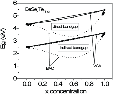
Figure 1: Direct and indirect bandgaps in BeSe_xTe_1-x : linear interpolation (full line); VCA (line with squares); BAC(diamonds); and interpolation to BAC model (dotted line).

We calculated also electronic and optical properties of a Si/BeSe_0.41Te_0.59 superlattice (SL) in (001) direction. Abrupt interface, flat band conditions were assumed. We adjusted the conduction band offset between BeSe_0.41Te_0.59 and Si at 1.2 eV as determined from electrical measurements Clark et al. (2000). Two interface subbands were found, one empty and one occupied within the Si bandgap. The origin of these interface subbands is due to polar nature of the interface or large difference between on-site energies of Si on the one side and Be or Se/Te on the other side.Saito and Ikoma (1992) In Fig. 2 we plot the joint density of states for vertical transitions in (Si${}_{2})_{4}$(BeSe_0.41Te${}_{0.59})_{4}$ SL. In such structures, due to band folding, the threshold of the direct bandgap is lowered for Si from 3.35 eV to 1 eV. The threshold is slightly below the fundamental bandgap of Si because of the two interface bands. Moreover, the first peak is wider. Si as an indirect bandgap semiconductor has two kinds of confined states in a quantum well Sandu et al. (2001), one given by the longitudinal valleys with an effective mass of 0.19m₀ and the other given by transverse valley with an effective mass of 0.91m₀. Hence the confined states that have a different first peak is made of the first states of both types of valley.

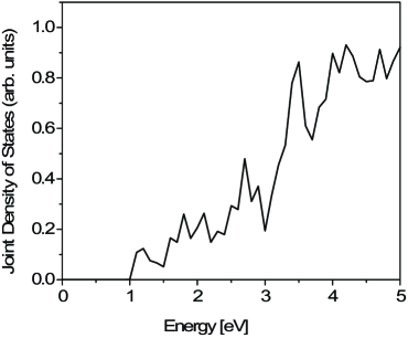
Figure 2: Joint density of states responsible for vertical transitions in Si/BeSe_xTe_1-x SL.

IV Conclusions

In conclusion, we extended the band anticrossing model to the empirical tight-binding theory. We used the Anderson model for impurity and a sp³ hybrid basis for zincblende structures within sp³s* Hamiltonian. The effective Hamiltonian of the alloy was obtained by impurity averaging and keeping only the terms responsible for energy shifts due to alloying. The pair impurity effects can easily be included as well. Thus no extra parameters are needed to calculate bandgaps.

The model was used for BeSe_1-xTe_x alloy. BeSe_1-xTe_x shows large band bowing, larger on the Se-rich side similar to ZnSeTe system. Bandgap was interpolated linearly between the two dilute limits. Further the model was applied to Si/BeSe_0.41Te_0.59 superlattice in (001) direction with abrupt interfaces. Due to polarity of the interface, two interface subbands are found within bandgap of Si. Also calculations show that the threshold for direct transitions is lowered in Si and that the absorption edge is slightly below the Si fundamental bandgap.