Intrinsic phonon decoherence and quantum gates in coupled lateral quantum dot charge qubits

Abstract

Recent experiments by Hayashi et al. [Phys. Rev. Lett. 91, 226804 (2003)] demonstrate coherent oscillations of a charge quantum bit (qubit) in laterally defined quantum dots. We study the intrinsic electron-phonon decoherence and gate performance for the next step: a system of two coupled charge qubits. The effective decoherence model contains properties of local as well as collective decoherence. Decoherence channels can be classified by their multipole moments, which leads to different low-energy spectra. It is shown that due to the super-Ohmic spectrum, the gate quality is limited by the single-qubit Hadamard gates. It can be significantly improved, by using double-dots with weak tunnel coupling.

I Introduction

In recent years, the experimental progress in analyzing transport properties in double quantum dots vanderWiel2 has lead to the fabrication of double dot structures with only one electron in the whole system Elzerman ; Andi . This well-defined situation permits, although it is strictly speaking not necessary Hayashi , to use quantum dot systems as quantum bits (qubits). In order to define qubits in lateral quantum dot (QD) structures, the two degrees of freedom, spin and charge, are naturally used. For spin qubits Loss , the information is encoded in the spin of a single electron in one quantum dot, whereas for the charge qubit Blick1 ; Leonid1 ; vanderWiel1 the position of a single electron in a double dot system defines the logical states. Similar ideas can also be applied to charge states in Silicon donors Hollenberg . Both realizations are interconnected: interaction and read-outElzerman of spin qubits are envisionedLoss to be all-electrical and to make use of the charge degree of freedom.

Although the promises of spin coherence in theoryLatestLoss and in bulk measurements Awschalom are tremendous in the long run, it was the good accessibility of the charge degrees of freedom which lead to a recent break-through Hayashi , namely the demonstration of coherent oscillations in a quantum dot charge qubit. In this experiment, three relevant decoherence mechanisms for these charge qubits have been pointed out: a cotunneling contribution, the electron-phonon coupling, and $1/f$-noise or charge noise in the heterostructure defining the dots.

Recent theoretical results UdoFrank predict that the cotunneling contribution can be very small, provided that the coupling between the dots and the connected leads is small. Thus, cotunneling is not a fundamental limitation. This, however, means that initialization and measurement protocols different from those of Ref. [Hayashi, ] are favorable Elzerman .

Other theoretical works Leonid2 ; Wu ; Vorojtsov ; Hu ; thorwart_mucciolo already describe the electron-phonon interaction for a single charge qubit in a GaAs/AlGaAs heterostructure. Moreover, also electronic Nyquist noise in the gate voltages affects the qubit system Marquardt . Note that the physics of the electron-phonon coupling is different and less limiting in the unpolar material Si Gorman , where the piezo-electric interaction is absent.

II Model

In this article, we analyze the decoherence due to the electron-phonon coupling in GaAs, which is generally assumed to be the dominant decoherence mechanism in a coupled quantum-dot setting. The recent experimental analysis shows that the temperature dependence of the dephasing rate in the experiment Hayashi can be modeled with the Spin-Boson model and hence is compatible with this assumption Leggett . We develop a model along the lines of Brandes et al. Brandes1 ; BrandesHabil to describe the piezo-electric interaction between electrons and phonons in lateral quantum dots. Thereby, we assume the distance between the two dots to be sufficiently large and the tunnel coupling $\Delta$ to be relatively small, which is a prerequisite for the validity of the model. The Hamiltonian for a system of two double dots with a tunnel-coupling within the double dots and electrostatic coupling between them, see Fig. 1, can be expressed as BrandesHabil

$$\hat{H}_{\rm total}=\hat{H}_{\rm sys}+\hat{H}_{\rm bath}+\hat{H}_{\rm int},$$ (1)

where

$$\hat{H}_{\rm sys} = -\sum_{i=1,2}\limits\frac{1}{2}\left(\varepsilon_{i}\hat{\sigma}_{z,i}+\Delta_{i}\hat{\sigma}_{x,i}\right)-k\hat{\sigma}_{z,1}\otimes\hat{\sigma}_{z,2}$$ (2)

$$\hat{H}_{\rm bath} = \sum_{q}\limits\hbar\omega_{q}c^{\dagger}_{q}c_{q}$$ (3)

refer to the qubits and the heat bath, respectively. $q$ is the phonon wave number. The system-bath interaction Hamiltonian $\hat{H}_{\rm int}$ depends on details of the setup such as the crystalline structure of the host semiconductor and the dot wave functions. We will distinguish between the two extreme cases of long correlation length phonons resulting in coupling of both qubits to a single phonon bath, or two distinct phonon baths for short phonon correlation length. The former case is more likely Ulbrich and applies to crystals which can be regarded as perfect and linear over the size of the sample, whereas the latter case describes systems that are vstrained or disordered and double quantum dots in large geometrical separation. The correlation length has to be distinguished from the wave length: The former indicates, over which distances the phase of the phonon wave is maintained,i.e., over which distance the description as a genuine standing wave applies at all, whereas the latter indicates the internal length scale of the wave.

II.1 One common phonon bath

In the case of a single phononic bath with a very long correlation length coupling to both charge qubits, $\hat{H}_{\rm int}$ can be written as

$$\hat{H}_{\rm int} = \sum_{q}\limits\frac{1}{2}\Big{[}(\alpha_{q,1}+\beta_{q,1}+\alpha_{q,2}+\beta_{q,2})\hat{\mathbf{1}}_{1}\otimes\hat{\mathbf{1}}_{2}+$$ (4)

$$+(\alpha_{q,1}-\beta_{q,1})\hat{\sigma}_{z,1}\otimes\hat{\mathbf{1}}_{2}+$$

$$+(\alpha_{q,2}-\beta_{q,2})\hat{\mathbf{1}}_{1}\otimes\hat{\sigma}_{z,2}\Big{]}(c^{\dagger}_{q}+c_{-q})\ .$$

The coefficients $\alpha_{q,i}$ and $\beta_{q,i}$ describe the coupling of a localized electron (one in each of the two double dot systems) to the phonon modes. They are given by

$$\alpha_{q,i} = \lambda_{q}\langle l,i|e^{i\vec{q}\vec{x}}|l,i\rangle,$$ (5)

$$\beta_{q,i} = \lambda_{q}\langle r,i|e^{i\vec{q}\vec{x}}|r,i\rangle,$$ (6)

where the $|l,i\rangle$ and $|r,i\rangle$ denote the wavefunctions of the electrons in the left or right dot of qubit $i$. We assume these wavefunctions to be two-dimensional Gaussians centered at the center of the dot, as sketched in Figure 1. These states approximate the ground state in the case of a parabolic potential and small overlap between the wavefunctions in adjacent dots. The coefficient $\lambda_{q}$ is derived from the crystal properties BrandesHabil .

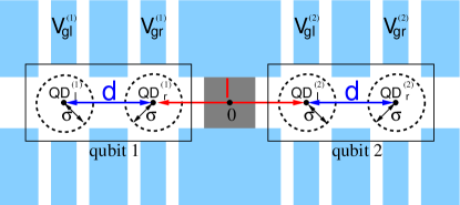
Figure 1: (Colour online) Sketch of the two coupled identical charge qubits realized in a lateral quantum dot structure. $d=100$ nm is the distance of the dot centers in one qubit, $l=200$ nm is the distance between the right dot center of qubit 1 and the left dot center of qubit 2. The width of the Gaussian wavefunction of an electron in each dot is $\sigma=5$ nm. The values chosen for the distances $d$ and $l$ are slightly smaller than in experimental realizations Hayashi ; Elzerman in order to provide a lower bound for the decoherence times. In principle, there could be tunneling processes between both qubits, i.e., the QDs two and three in the chain, but we assume that the coupling is pinched off by applying appropriate gate voltages. The gray box between the qubits indicates that there is no tunneling between the qubits.

Henceforth, we investigate the case of two identical qubits. Due to the fact that the relevant distances are arranged along the $x$-direction, we obtain the coupling coefficients

$$\alpha_{q,1} = \lambda_{q}e^{iq\left(-{l}/{2}-d\right)}e^{-{q^{2}\sigma^{2}}/{4}},$$ (7)

$$\beta_{q,1} = \lambda_{q}e^{-{iql}/{2}}e^{-{q^{2}\sigma^{2}}/{4}},$$ (8)

$$\alpha_{q,2} = \lambda_{q}e^{{iql}/{2}}e^{-{q^{2}\sigma^{2}}/{4}},$$ (9)

$$\beta_{q,2} = \lambda_{q}e^{iq\left({l}/{2}+d\right)}e^{-{q^{2}\sigma^{2}}/{4}}\ .$$ (10)

Here, $q$ is the absolute value of the wavevector $\vec{q}$. The second exponential function in each line is the overlap between the two Gaussian wavefunctions.

This two-qubit bath coupling Hamiltonian is quite remarkable, as it does not fall into the two standard categories usually treated in literature (see, e.g., Refs. [Kempe, ; Zanardi, ; pra_markus, ] and references therein): On the one hand, there is clearly only one bath and each qubit couples to the bath modes with matrix elements of the same modulus, so the noise between the qubits is fully correlated. On the other hand, the Hamiltonian does not obey the familiar factorizing collective noise form $\hat{H}_{\mathrm{SB,coll}}=\hat{X}_{\rm system}\otimes\hat{X}_{\rm bath}$. Such a form would lead to a high degree of symmetry and thus protection from the noise coupling Zanardi ; Kempe , however, the Hamiltonian $H_{\rm int}$, eq. 4, cannot be factorized in such a bilinear form. It is hence intriguing to explore where in between these cases the physics ends up to be. This is in particular important for finally finding strategies to protect the qubits against decoherence, and for estimating the scaling of decoherence in macroscopic quantum computers.

In order to obtain the dynamics of the reduced density matrix $\rho$ for the coupled qubits, i.e., for the degrees of freedom that remain after the environment is traced out, we apply Bloch-Redfield theory Agyres ; Weiss ; Hartmann . It starts out from the Liouville-von Neumann equation $i\hbar\dot{\rho}=[\hat{H},\rho_{\mathrm{tot}}]$ for the total density operator. A perturbational treatment of the system-bath coupling Hamiltonian $\hat{H}_{\mathrm{int}}$ results in the master equation

$$\dot{\rho}=-\frac{i}{\hbar}[\hat{H}_{\mathrm{sys}},\rho]-\frac{1}{\hbar^{2}}\int_{0}^{\infty}\!\!\!d\tau\ \mbox{tr}_{B}[\hat{H}_{\mathrm{int}},[\tilde{H}_{\mathrm{int}}(-\tau),\rho\otimes\rho_{B}]],$$ (11)

where $\rho_{B}=\exp(-\beta\hat{H}_{B})/Z$ denotes the equilibrium density matrix of the bath. Evaluating the trace over all bath variables, $\mbox{tr}_{B}$, and decomposing the reduced density operator into the eigenbasis of the unperturbed system Hamiltonian, we obtain Blum ; Weiss

$$\dot{\rho}_{nm}=-i\omega_{nm}\rho_{nm}-\sum_{k,\ell}R_{nmk\ell}\rho_{k\ell},$$ (12)

where $\omega_{nm}=E_{n}-E_{m}$. The first term on the right hand side describes the unitary evolution and the Redfield relaxation tensor $R_{nmk\ell}$ incorporates the decoherence effects. It is given by

$$R_{nmk\ell}=\delta_{\ell m}\sum_{r}\Gamma^{(+)}_{nrrk}+\delta_{nk}\sum_{r}\Gamma^{(-)}_{\ell rrm}-\Gamma^{(-)}_{\ell mnk}-\Gamma^{(+)}_{\ell mnk}\textrm{,}$$ (13)

where the rates $\Gamma^{(\pm)}$ are determined by Golden Rule expressionsBlum ; Weiss , see Eqs. (20) and (21), below. The Redfield tensor and the time evolution of the reduced density matrix are evaluated numerically to determine the decoherence properties of the system due to a weak electron-phonon coupling. Note that in addition, Ohmic electronic noise can be taken into account by employing the spectral functiongovernale $J_{\Sigma}(\omega)=J_{\rm Ohmic}(\omega)+J(\omega)$, where $J(\omega)$ contains only the phonon contribution. It is also possible to take $1/f$-noise in the quantum dot system into account in the same way. The $1/f$-noise essentially determines the magnitude of the dephasing part of the decoherence. Thus, it is in turn possible to impose for the zero frequency component $J(0)$ the experimental value of the dephasing rates or a value from a microscopic model Falci . However, in many cases it turns out to be non-Markovian and/or non-Gaussian, leading to non-exponential decay, which can neither be described by Bloch-Redfield theory nor parameterized by a single rate.

In order to compute the rates, the electron-phonon interaction Hamiltonian has first to be taken from the localized representation to the computational basis, which is straightforward. To compute Bloch-Redfield rates, it is necessary to rotate into the eigenbasis of the system. After this basis change, the spectral densities $J_{\ell mnk}(\omega)$ are calculated along the lines of Ref. [BrandesHabil, ] as

$$J_{\ell mnk}(\omega)=\langle\left(B^{-1}CB\right)_{\ell m}\left(B^{-1}CB\right)_{nk}\rangle_{q},$$ (14)

where $B$ is the matrix for the basis transformation from the computational basis {$|00\rangle$, $|01\rangle$, $|10\rangle$, $|11\rangle\}$ to the eigenbasis of the system and $\langle\cdot\rangle_{q}$ denotes an averaging over all phonon modes $q$ with frequency $\omega$. The matrix $C$ is diagonal in the computational basis, $C={\rm diag}(\alpha_{q,1}-\beta_{q,1}+\alpha_{q,2}-\beta_{q,2},\alpha_{q,1}-\beta_{q,1}+\alpha_{q,2}-\beta_{q,2},\alpha_{q,1}-\beta_{q,1}+\alpha_{q,2}-\beta_{q,2},\alpha_{q,1}-\beta_{q,1}+\alpha_{q,2}-\beta_{q,2})$.

The explicit derivation shows that it is most convenient to split the total spectral function $J_{\ell mnk}(\omega)$ [see Eq. (14)] into odd and even components

$$J_{\ell mnk}(\omega)=e_{\ell mnk}J_{e}(\omega)+o_{\ell mnk}J_{o}(\omega)\ ,$$ (15)

where the prefactors $e_{\ell mnk}$ and $o_{\ell mnk}$ of the even/odd part of the spectral function are matrix elements coming from the basis change from the computational basis to the eigenbasis of the system and

$$J_{e/o}(\omega)=\frac{\pi}{4}\sum_{q}|\alpha_{q,1}-\beta_{q,1}\pm\alpha_{q,2}\mp\beta_{q,2}|^{2}\delta(\omega-\omega_{q}).$$ (16)

They evaluate to

$$J_{e,o}(\omega)=\frac{\pi\hbar\omega g}{4}\Bigg{[}2-2\frac{\omega_{d}}{\omega}\sin\left(\frac{\omega}{\omega_{d}}\right)\mp\frac{\omega_{l}}{\omega}\sin\left(\frac{\omega}{\omega_{l}}\right)\pm 2\frac{\omega_{l+d}}{\omega}\sin\left(\frac{\omega}{\omega_{l+d}}\right)\mp\frac{\omega_{l+2d}}{\omega}\sin\left(\frac{\omega}{\omega_{l+2d}}\right)\Bigg{]}e^{-{\omega^{2}}/{2\omega_{c}^{2}}},$$ (17)

where $g=0.05$ is the dimensionless electron-phonon coupling strength for the commonly used material GaAs Brandes1 ; BrandesHabil and $c_{S}$ the speed of sound. The different frequencies represent the distances in the system: $\omega_{d}=c_{s}/d$, $\omega_{l}=c_{s}/l$, $\omega_{d+l}=c_{s}/(d+l)$ and $\omega_{2d+l}=c_{s}/(2d+l)$, and $\omega_{c}=c_{s}/\sigma$. This structure can be understood as follows: The electron-phonon interaction averages out if the phonons are rapidly oscillating within a dot, i.e. if the wavelength is much shorter than the dot size — this provides the high-frequency cutoff at $\omega_{c}$. On the other hand, long-wavelength phonons do not contribute to decoherence between dots $i$ and $j$, if the wavelength is much longer than their separation because then, the energy shift induced by the phonon displacement will only lead to a global phase. Furthermore, we can approximate the leading order at low frequencies as

$$J_{e}(\omega) = \frac{2\pi\hbar gd^{2}}{3c_{s}^{2}}\omega^{3}+\mathcal{O}(\omega^{5}),$$ (18)

$$J_{o}(\omega) = \frac{\pi\hbar g(l^{2}d^{2}+2ld^{3}+d^{4})}{10c_{s}^{4}}\omega^{5}+\mathcal{O}(\omega^{7}).$$ (19)

This different power-laws $\omega^{3}$ to $\omega^{5}$ can be understood physically as illustrated in Figure 2.

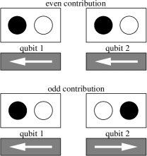
Figure 2: Illustration of the even (top) and odd (bottom) contributions to the total rates. Filled circles indicate occupied dots. For long-wavelength modes, the energy shifts induced by underlying phonons in the two dots add up coherently in the even case but cancel in the odd case. Note, that moving charges from the black to the white dots changes the dipole moment in the even but not in the odd case.

“Even” terms are the natural extension of the one-qubit electron-phonon coupling, adding up coherently between the two dots. In the “odd” channel, the energy offset induced in one qubit is, for long wavelengths, cancelled by the offset induced in the other qubit. Thus, shorter wavelenghts are required for finding a remaining net effect. An alternative point of view is the following: The distribution of the two charges can be parameterized by a dipole and a quadrupole moment. The “even” channel couples to the dipole moment of the charge configuration similar to the one-qubit case. The “odd” channel couples to the quadrupole moment alone (see Figure 2). Thus, it requires shorter wavelengths and consequently is strongly supressed at low frequencies. This explains the different low-frequency behavior illustrated for realistic parameters in Figure 3.

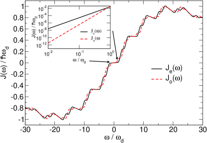
Figure 3: (Colour online) Spectral functions $J_{e,o}(\omega)$ in the case of one common phonon bath for the fixed parameters $c_{s}=5000$ m/s, $g=0.05$, $d=100$ nm, $l=200$ nm and $\sigma=5$ nm. Inset: zoom for small frequencies.

Thus, we can conclude that for small frequencies the odd processes are suppressed by symmetry — even beyond the single-dot supression and the suppression of asymmetric processes.

With these expressions for the spectral densities, one can proceed as in Ref. [pra_markus, ] and determine the rates that constitute the Redfield tensor to read

$$\Gamma^{(+)}_{\ell mnk} = \frac{J_{\ell mnk}(\omega_{nk})}{2\hbar}\left[\coth\left(\frac{\hbar\omega_{nk}}{2k_{B}T}\right)-1\right],$$ (20)

$$\Gamma^{(-)}_{\ell mnk} = \frac{J_{\ell mnk}(\omega_{\ell m})}{2\hbar}\left[\coth\left(\frac{\hbar\omega_{\ell m}}{2k_{B}T}\right)+1\right].$$ (21)

For $\omega_{ij}\rightarrow 0$, these rates vanish due to the super-Ohmic form of the bath spectral function. From this, we find the time evolution of the coupled qubit system and finally also the gate quality factors.

II.2 Two distinct phonon baths

When each qubit is coupled to its own phononic bath, the part of the Hamiltonian that describes the interaction with the environment $H_{\rm int}$ is given by

$$\hat{H}_{\rm int} = \sum_{q_{1}}\limits\frac{1}{2}\Big{[}(\alpha_{q_{1}}+\beta_{q_{1}})\hat{\mathbf{1}}_{1}+(\alpha_{q_{1}}-\beta_{q_{1}})\hat{\sigma}_{z,1}\Big{]}$$ (22)

$$\times(c^{\dagger}_{q_{1}}+c_{-q_{1}})\otimes\hat{\mathbf{1}}_{2}+$$

$$+\sum_{q_{2}}\limits\frac{1}{2}\Big{[}(\alpha_{q_{2}}+\beta_{q_{2}})\hat{\mathbf{1}}_{2}+(\alpha_{q_{2}}-\beta_{q_{2}})\hat{\sigma}_{z,2}\Big{]}$$

$$\times(c^{\dagger}_{q_{2}}+c_{-q_{2}})\otimes\hat{\mathbf{1}}_{1}\ .$$

This scenario can be realized in different ways: One can split the crystal into two pieces by an etched trench. Alternatively, if there is lattice disorder and/or strong nonlinear effects, the phonons between the dots may become uncorrelated.

The calculation of the coupling coefficients works in a similar way, but there are two different indices $q_{1}$ and $q_{2}$ to represent the phononic baths of each qubit

$$\alpha_{q_{1}} = \lambda_{q_{1}}e^{iq_{1}\left(-{l}/{2}-d\right)}e^{-{q_{1}^{2}\sigma^{2}}/{4}},$$ (23)

$$\beta_{q_{1}} = \lambda_{q_{1}}e^{-{iq_{1}l}/{2}}e^{-{q_{1}^{2}\sigma^{2}}/{4}},$$ (24)

$$\alpha_{q_{2}} = \lambda_{q_{2}}e^{{iq_{2}l}/{2}}e^{-{q_{2}^{2}\sigma^{2}}/{4}},$$ (25)

$$\beta_{q_{2}} = \lambda_{q_{2}}e^{iq_{2}\left({l}/{2}+d\right)}e^{-{q_{2}^{2}\sigma^{2}}/{4}}\ .$$ (26)

The expression for the spectral functions $J_{\ell mnk}(\omega)$ turns out to be exactly the same as the one in the last section with the only difference that instead of $\alpha_{q,i}$, the coupling between electrons and phonons is now expressed as $\alpha_{q_{i}}$ (with $i=1,2$ for both qubits). Therefore, in order to obtain the spectral density $J_{\ell mnk}(\omega)$, one has to average over two distinct baths, i.e.

$$J_{\ell mnk}(\omega)=\langle\left(B^{-1}CB\right)_{\ell m}\left(B^{-1}CB\right)_{nk}\rangle_{q_{1},q_{2}}.$$ (27)

Again, we find two different functions that we name in the same way as in the previous section, $J_{e}(\omega)$ and $J_{o}(\omega)$, which are given by

$$J_{e,o}(\omega)=\frac{\pi\hbar\omega g}{4}\Bigg{[}2-2\frac{\omega_{d}}{\omega}\sin\left(\frac{\omega}{\omega_{d}}\right)\mp 2\left(\frac{\omega_{\frac{l}{2}}}{\omega}\sin\left(\frac{\omega}{\omega_{\frac{l}{2}}}\right)-\frac{\omega_{d+\frac{l}{2}}}{\omega}\sin\left(\frac{\omega}{\omega_{d+\frac{l}{2}}}\right)\right)^{2}\Bigg{]}e^{-{\omega^{2}}/{2\omega_{c}^{2}}}\ .$$ (28)

The prefactors from the basis change also enter the expressions for the rates in the same way as in the last section.

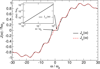
Figure 4: (Colour online) Spectral functions $J_{e,o}(\omega)$ in the case of two distinct phonon baths for the fixed parameters $c_{s}=5000$ m/s, $g=0.05$, $d=100$ nm, $l=200$ nm and $\sigma=5$ nm. Inset: magnification for small frequencies.

The spectral functions $J_{e,o}(\omega)$ are plotted in Figure 4; the inset depicts the proportionality to $\omega^{3}$ for small frequencies.

III Golden Rule Rates

We proceed as in Ref. [pra_markus, ] and determine the Golden rule rates that govern the Redfield tensor. Thereby, we find both the time evolution of the coupled system and the gate quality factors.

Let us first discuss the impact of this particular bath coupling on the dephasing and relaxation rates. The decoherence rates, i.e., the relaxation and dephasing rates, are defined according to $\Gamma_{R}=-\sum_{n}\Lambda_{n}$, where $\Lambda_{n}$ are the eigenvalues of the matrix composed of the elements $R_{n,n,m,m}$, $n,m=1,\ldots,4$, and $\Gamma_{\varphi_{nm}}=-\mbox{Re}R_{n,m,n,m}$ for non-degenerate levels $|\omega_{nm}|>|R_{n,m,n,m}|$ and in the absence of Liouvillian degeneracy, $|\omega_{nm}-\omega_{kl}|>|R_{a,b,c,d}|\quad a,b,c,d,\in\{k,l,m,n\}$, respectively governale .

As a reference point, we study the rates in the uncoupled case. In this case, and in the absence of degeneracies between the qubits, there is a clear selection rule that the environment only leads to single-qubit processes, i.e., decoherence can be treated at completely separate footing. As a result, all rates are identical between the qubits. To make this obvious, we rewrite the original Hamiltonian in the one-bath case, combining Eq. (4) with eqs. (7)–(10) as

$$\hat{H}_{\rm int} = \sum_{q}\limits\Bigg{[}-2ie^{-q^{2}\sigma^{2}/4}\sin\left(\frac{qd}{2}\right)\Big{(}e^{-iq(l+d)/2}\hat{\sigma}_{z,1}+$$ (29)

$$+e^{iq(l+d)/2}\hat{\sigma}_{z,2}\Big{)}+E_{0}\hat{\mathbf{1}}\Bigg{]}\left(c^{\dagger}_{q}+c_{-q}\right)$$

which — besides a phase factor which is meaningless for single-qubit transitions — is identical to the standard electron-phonon Hamiltonian for double dots BrandesHabil .

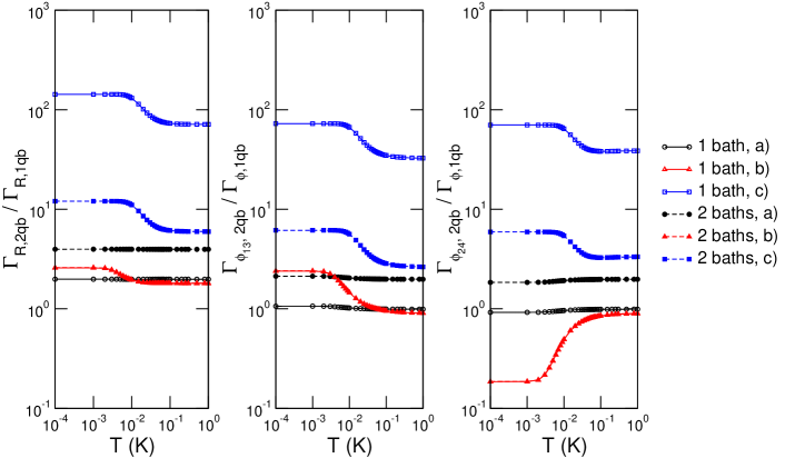
Figure 5: (Colour online) Temperature dependence of the relaxation and dephasing rates normalized by the single-qubit relaxation and dephasing rates. The two-qubit relaxation rate is given by the trace of the relaxation part of the Redfield tensor in secular approximation. The energy scales for the two-qubit transitions $1\leftrightarrow 3$ and $2\leftrightarrow 4$ are comparable to the single qubit energy scale, the characteristic qubit energies are $E_{s}=(1/8)$ GHz. The different cases are (a) $\varepsilon_{1}=\Delta_{1}=(1/40)E_{s}$, $\varepsilon_{2}=\Delta_{2}=-(21/40)E_{s}$, and coupling energy $K=0$, (b) $\varepsilon_{1}=\Delta_{1}=-(1/2)E_{s}$, $\varepsilon_{2}=\Delta_{2}=-(21/40)E_{s}$, and $K=0$), and (c) $\varepsilon_{1}=\Delta_{1}=-(1/2)E_{s}$, $\varepsilon_{2}=\Delta_{2}=-(1/2)E_{s}$ and $K=10E_{s}$. Note that cases (a) and (b) model uncoupled qubits, especially for case (a) the overall relaxation rate for the two-qubit system is approximately twice the single-qubit relaxation rate when calculated for the dominating larger energy scale of the two-qubit system ($\varepsilon_{2}=\Delta_{2}=-(21/40)E_{s}$).

Figure 5 shows the temperature dependence of the energy relaxation rate $\Gamma_{R}$ and the two dephasing rates $\Gamma_{\phi_{13}}$ and $\Gamma_{\phi_{24}}$ compared to the single qubit relaxation and dephasing rates. In this notation, $\Gamma_{\phi_{ij}}$ is the rate at which a superposition of energy eigenstates $i$ and $j$ is decays into a classical mixture. We considered the following three cases, characterized by values on the matrix element relative to a characteristic system energy scale $E_{s}$: (a) large difference of the $\varepsilon_{i}$ and $\Delta_{i}$ ($i=1,2$) between both qubits and no coupling between the qubits ($\varepsilon_{1}=\Delta_{1}=(1/40)E_{s}$, $\varepsilon_{2}=\Delta_{2}=-(21/40)E_{s}$ and coupling energy $K=0$), (b) small asymmetry between the parameters for both qubits and no coupling ($\varepsilon_{1}=\Delta_{1}=-(1/2)E_{s}$, $\varepsilon_{2}=\Delta_{2}=-(21/40)E_{s}$ and $K=0$), and (c) without asymmetry between the qubits and a rather strong coupling between the qubits ($\varepsilon_{1}=\Delta_{1}=-(1/2)E_{s}$, $\varepsilon_{2}=\Delta_{2}=-(1/2)E_{s}$ and $K=10E_{s}$). One generally would expect a different value of the distance between the dot centers in the qubits $d$, when the tunneling coupling is varied. However, in our case of the dot wavefunctions which overlap only in their Gaussian tails, this effect is very small (below $1$ nm for a change in the tunneling amplitude $\Delta$ of approximately $\sim(1/2)E_{s}$) for the lengthscales that we are considering. Note, that in Ref. Andi, a substantial change of $\Delta$ over more than an order of magnitude was obtained experimentally by a rather mild adjustment of the gate voltage, so it is consistent that a small change of $\Delta$ can be achieved by a tiny adjustment. Therefore the value $d=100$ nm is used for the electron-phonon coupling encoded in $J_{e}$ and $J_{o}$ in all cases.

For case (a), we find that all rates are for all temperatures larger than the single qubit rates, as one would expect Duer . In more detail, for the single bath case, the ratio of the relaxation rates is approximately $1.9$, the ratio of the single-qubit dephasing rate and the two-qubit dephasing rate $\Gamma_{\phi_{24}}$ is around $0.9$ and for the dephasing rate $\Gamma_{\phi_{13}}$, the ratio is $1.0$. The behaviour of the even and odd parts of the spectral function in the single bath case can be explained from the spectral function Fig. 3, for small $\omega$ one finds that $J_{o}<J_{e}$. For the case of large frequencies, however, the even part of the spectral functionincreases and even dominate beyond the threshold $\omega\gtrsim\omega_{d}$. Overall, it is found that in the case of a single-bath the decoherence effects are significantly suppressed compared to the two-bath scenario. For the two-bath case, the ratios are for the relaxation rates approximately $3.9$, for the dephasing rate $\Gamma_{\phi_{24}}$ around $1.9$ and for the dephasing rate $\Gamma_{\phi_{13}}$ it is $2.0$. Note that for the two-bath case $J_{e}<J_{o}$ always and for the case where both tunnel matrix elements in the Hamiltonian vanish, the rate vanishes, too.

After decreasing the asymmetry between the two qubits as in case (b), the rates decreased but are still comparable with the single qubit rates, besides the last dephasing rate $\Gamma_{\phi_{24}}$. This can be understood, if one considers the energy spectrum of the eigenvalues of the system Hamiltonian. In cases (a) and (b) there is significant difference between the qubits, so it is straightforward to map the two-qubit rates onto the corresponding single qubit rates and they are largely determined by single-qubit physics. In case (c), we consider a fully symmetric case in the qubit parameters, but with a finite and large coupling between the qubits. This coupling lifts the degeneracy but makes the rate a generic two-qubit rate which belongs to a relatively robust transition with small transition matrix elements for the single bath case. At high temperatures, these symmetry-related effects wash out as discussed in Ref. [Praktikanten, ]. However, the high-temperature rates do not coincide with the single-qubit rates, as the underlying energy scales are still different and in generally larger for the two-qubit situation.

Overall, the ratio of the two-qubit and single-qubit relaxation rates decreases for increasing temperature due to the reduction of correlation effects in the double dot system, besides case c), where a symmetry based on the underlying Hamiltonian becomes important.

IV Quantum gate performance

For the characterization of the quantum gate performance of this two-qubit system, it is necesssary to introduce suitable quantifiers. Commonly, one employs the four gate quality factors introduced in Ref. [pcz, ]; fidelity $\mathcal{F}$, purity $\mathcal{P}$, quantum degree $\mathcal{Q}$, and entanglement capability $\mathcal{C}$ to chararcterize a gate operation within a hostile enviroment.

The fidelity, i.e., the overlap between the ideal propagator and the simulated time evolution including the decoherence effects, is defined as

$$\mathcal{F}=\overline{\bra{\Psi_{\rm in}}\hat{U}^{\dagger}\rho_{\rm out}\hat{U}\ket{\Psi_{\rm in}}}\textrm{,}$$ (30)

where the bar indicates an average over a set of 36 unentangled input states $\ket{\Psi_{\rm in}}=\ket{\psi_{i}}\ket{\psi_{j}}$, with $i,j=1,\ldots,6$. The 6 single-qubit states $\ket{\psi_{i}}$ are chosen such that they are symmetrically distributed over the Bloch sphere,

$$\ket{\psi_{1}}=\ket{0},\quad\ket{\psi_{2}}=\ket{1},\quad\ket{\psi_{3,\ldots,6}}=\frac{\ket{0}+e^{i\phi}\ket{1}}{\sqrt{2}}$$ (31)

where $\phi=0,\pi/2,\pi,3\pi/2$. Here, $\hat{U}$ is the ideal unitary time evolution for the given gate, and $\hat{\rho}_{\rm out}$ is the reduced density matrix resulting from the simulated time evolution. A perfect gate reaches a fidelity of unity. The purity $\mathcal{P}$ measures the strength of the decoherence effects,

$$\mathcal{P}=\overline{\mbox{tr}(\rho_{\rm out}^{2})}\textrm{.}$$ (32)

Again, the bar indicates the ensemble average. A pure state returns unity and for a mixed state the purity can drop to a minimum given by the inverse of the dimension of the system Hilbert space, i.e. 1/4 in our case.

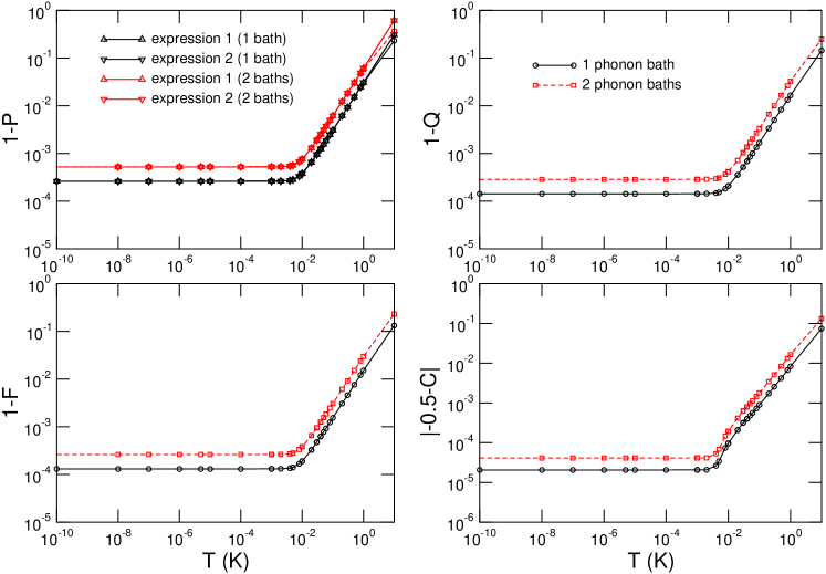
Figure 6: (Colour online) Temperature dependence of the deviation of the four gate quality factors from their ideal values for the cnot gate. The decoherence due to phonons is taken into account. The black line shows the results for a single phonon bath and the red line is for two phononic baths. The characteristic qubit energies are $E_{s}=1/4$ GHz and the tunnel amplitudes are $\Delta_{i}=E_{s}$ ($i=1,2$) due to the spacing of the double dots. In the curves for the deviation of the purity, we included lines for the analytical expressions 1 from Eq. (34) and 2 from Eq. (39).

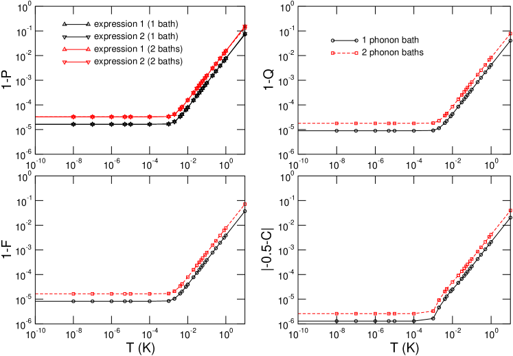
Figure 7: (Colour online) Temperature dependence of the deviation of the four gate quality factors from their ideal values for the cnot gate. The decoherence due to phonons is taken into account. The black line shows the results for a single phonon bath and the red line is for two phonon baths. The characteristic qubit energies are $E_{s}=1/4$ GHz and the tunnel amplitude during the Hadamard operation on the second qubit is $\Delta_{2}=1/4E_{s}$, i.e., a factor $4$ smaller than in Figure 6. In the curves for the deviation of the purity, we included lines for the analytical expressions 1 from Eq. (34) and 2 from Eq. (39).

If the density operator $\rho$ describes an almost pure state, i.e., if the purity is always close to the ideal value 1, it is possible to estimate the purity loss during the gate operation from its decay rate along the lines of Ref. [Fonseca04, ]. Thereby, one first evaluates the decay of $(d/dt)\mbox{tr}\rho^{2}$ for an arbitrary pure qubit state $\rho=|\psi\rangle\langle\psi|$. From the basis-free version of the master equation (11), follows straightforwardly

$$\frac{d}{dt}\mbox{tr}\rho^{2}=-\frac{2}{\hbar^{2}}\int_{0}^{\infty}d\tau\ \mbox{tr}_{S+B}[\hat{H}_{\mathrm{int}},[\tilde{H}_{\mathrm{int}}(-\tau),\rho\otimes\rho_{B}]]\rho\textrm{.}$$ (33)

By tracing out the bath variables, we obtain an expression that contains only qubit operators and bath correlation functions. This depends on the state $|\psi\rangle$ via the density operator. Performing the ensemble average over all pure states as described in the Appendix A, we obtain

$$\dot{\mathcal{P}}=\frac{2}{\hbar^{2}(N+1)}\int_{0}^{\infty}d\tau\ \mbox{tr}\langle[\hat{H}_{\mathrm{int}},\tilde{H}_{\mathrm{int}}(-\tau)]_{+}\rangle_{B,\mathrm{eq}},$$ (34)

where $N=4$ denotes the dimension of the system Hilbert space of the two qubits. We have used the fact that $\mbox{tr}\hat{H}_{\mathrm{int}}=0$. Although the discrete and set of states employed in the numerical computation is obviously different from the set of all pure states, we find that both ensembles provide essentially the same results for the purity.

If the bath couples to a good quantum number, i.e., for $[\hat{H}_{\mathrm{sys}},\hat{H}_{\mathrm{int}}]=0$, the system operator contained in the interaction picture operator $\tilde{H}_{\mathrm{int}}(-\tau)$ remains time-independent. Then, the $\tau$-integration in (34) is effectively the Fourier transformation of the symmetrically ordered bath correlation function in the limit of zero frequency. Thus, we obtain

$$\dot{\mathcal{P}}=-\frac{2}{N+1}\lim_{\omega\to 0}\sum_{i}J_{i}(\omega)\coth\frac{\hbar\omega}{2kT},$$ (35)

where

$$J_{i}(\omega)=\frac{\pi}{4}\sum_{q}|\alpha_{q,i}-\beta_{q,i}|^{2}\delta(\omega-\omega_{q})$$ (36)

denotes the spectral density of the coupling between qubit $i$ and the heat bath(s).

In the present case of a super-Ohmic bath, the limit $\omega\to 0$ results for the coupling to a good quantum number in $\dot{\mathcal{P}}=0$. This means that whenever the tunnel coupling in the Hamiltonian (2) is switched off, i.e. for $\Delta_{1}=\Delta_{2}=0$, the purity decay rate vanishes. Thus, we can conclude that the significant purity loss for the cnot operation studied below [cf. Eq. (IV)], stems from the Hadamard operation. This is remarkably different from cases with other bath spectra: For an ohmic bath, for which $J_{i}(\omega)\propto\omega$, expresion (35) converges in the limit $\omega\to 0$ to a finite value. By contrast, for a sub-ohmic bath, this limit does not exist and, consequently, the purity decay cannot be estimated by its decay rate. During the stage of the Hadamard operation, $\Delta_{2}=\Delta$ while $\Delta_{1}=0$. Then, the interaction picture versions of the qubit-bath coupling operators read

$$\tilde{\sigma}_{z,1}(-\tau) = \hat{\sigma}_{z,1},$$ (37)

$$\tilde{\sigma}_{z,2}(-\tau) = \hat{\sigma}_{z,2}\cos(\Delta\tau/\hbar)-\hat{\sigma}_{y,2}\sin(\Delta\tau/\hbar).$$ (38)

In the case where both qubits couple to individual environments, the expression for the change of the purity can be evaluated for each qubit separately. For qubit 2, we still have a coupling to a good quantum number, while for qubit 1, the appearence of $\cos(\Delta\tau/\hbar)$ results in a Fourier integral evaluated at the frequency $\Delta/\hbar$. Thus, we finally obtain

$$\dot{\mathcal{P}}=-\frac{4kT}{5}\lim_{\omega\to 0}\frac{J_{1}(\omega)}{\hbar\omega}-\frac{1}{5}J_{2}(\Delta/\hbar)\coth\frac{\Delta}{2kT}.$$ (39)

For the super-Ohmic bath under consideration [see eqs. (18) and (19)], the first term in Eqn. (39) vanishes.

In the case of one common heat bath, the estimate of the purity decay is calculated in the same way. The only difference is that we have to consider, in addition, cross terms of the type $\hat{\sigma}_{1,z}\otimes\hat{\sigma}_{2,z}$, i.e. terms that contain operators of different qubits. The contribution of these terms, however, vanishes when performing the trace over the bath variables in Eq. (34). Thus, we can conclude that within this analytical estimate, the purity decay rate is identical for both the individual bath model and the common bath model.

The so-called quantum degree

$$\mathcal{Q}=\max_{\rho_{\rm out},\ket{\Psi_{\rm me}}}\bra{\Psi_{\rm me}}\rho_{\rm out}\ket{\Psi_{\rm me}}$$ (40)

is the overlap of the state obtained after the simulated gate operation and the maximally entangled Bell states. Finally the entanglement capability $\mathcal{C}$ is defined as the smallest eigenvalue of the density matrix resulting from transposing the partial density matrix of one qubit. As shown in Ref. [peres, ], the non-negativity of this smallest eigenvalue is a necessary condition for the separability of the density matrix into two unentangled systems. The entanglement capability approaches $-0.5$ for the ideal cnot gate.

It has been shown that the controlled-NOT (cnot) gate together with single-qubit operations is sufficient for universal quantum computation. Here, we investigate the decoherence during a cnot gate which generates maximally entangled Bell states from unentangled input states. In Figures 6 and 7 the simulated gate evolution in the presence of phonon baths is shown. Using the system Hamiltonian, the cnot gate can be implemented through the following sequence of elementary quantum gates thorwart ; pra_markus

$$U_{\rm CNOT} = U_{\rm H}^{(2)}\exp\left(-i\frac{\pi}{4}\hat{\sigma}_{z,1}\right)\exp\left(-i\frac{\pi}{4}\hat{\sigma}_{z,2}\right){}\times$$

$${}\times\exp\left(-i\frac{\pi}{4}\hat{\sigma}_{z,1}\hat{\sigma}_{z,2}\right)\exp\left(-i\frac{\pi}{2}\hat{\sigma}_{z,1}\right)U_{\rm H}^{(2)}\textrm{, }\quad$$

where $U_{\rm H}^{(2)}$ denotes the Hadamard gate operation performed on the second qubit. This gate sequence just involves one two-qubit operation at step three. The parameters for the numerical calculations are given below Figs. 6 and 7.

In Fig. 6, the gate quality factors for the case of a single or two distinct phononic baths are shown. It is observed that for the case of a single phonon bath they achieve better values. This offset is due to the larger number of non-vanishing matrix elements in the coupling of the noise to the spin components for the two bath case. Here, due to several non-commuting terms in the coupling to the bath and the different Hamiltonians needed to perform the individual steps of the quantum gate, the gate quality factors saturate when the temperature $T$ is decreased. This happens at around $T=T_{s}=12$ mK corresponding to $E_{s}=1/4$ GHz as the characteristic energy scale.

Figure 7, depicts the same behaviour of the gate quality factors as in Figure 6 with the only difference that the tunnel coupling $\Delta_{2}$ is smaller by a factor of $4$ during the Hadamard operation. The qualitative behavior is very similar to that in Figure 6, but the deviation from the ideal values for the gate quality factors is much smaller and already fulfills the criterion of an allowed deviation of $10^{-4}$. The reduction of the tunnel amplitudes by a factor $4$ corresponds to a very small change of the distance $d$ in the two qubits (namely, from $100.0$ nm to $100.3$ nm) owing to the Gaussian shape of the electron wavefunctions, provided their distance is sufficiently large BrandesHabil .

We have already mentioned that the phonon contribution to decoherence still allows for the fidelity values below the threshold $1-F<10^{-4}$ from Ref. [DiVincenzo, ]. For a reliable quantum computer, however, such intrinsic decoherence mechanisms should beat the threshold at least by an order of magnitude. This can be achieved as follows: As we have seen, the Hadamard gate is the step limiting the performance as during the Hadamard the system is vulnerable against spontaneous emission at a rate $\gamma\propto E^{3}$, where $E$ is the typical energy splitting of the single qubit. The duration of the Hadamard, on the other hand, scales as $\tau\propto 1/E$. Thus, the error probability and the purity decay reduces to $1-e^{-\gamma\tau}\simeq\gamma\tau\propto E^{2}$. Thus, by making the Hadamard slower, i.e., by working with small tunnel couplings between the dots, the gate performance can be increased. This works until Ohmic noise sources, electromagnetic noise on the gates and controls, takes over. This is demonstrated nicely in Fig. 7, where the cnot gate for a modified Hadamard opertation (on the second qubit) with $\Delta_{2}=\varepsilon_{2}=(1/4)E_{s}$ is depicted. It is clearly observed that by decreasing the tunnel matrix element and by increasing the evolution time the decoherence is reduced and the threshold for the gate quality factors to allow universal quantum computation Aharonov can be achieved.

The gate quality of a CNOT under decoherence has been studied in Refs. [thorwart, ; pra_markus, ] for standard collective and/or single-qubit noise in Ohmic environments. The single-qubit case for charge qubits in GaAs has been studied in Ref. [thorwart_mucciolo, ] with emphasis on non-Markovian effects. Even in view of this, and in view of the emphasis of the strong tunneling regime, that work arrives at the related conclusion that intrinsic phonon decoherence in this system can be limited. Please note, that the approximations in the microscopic model give an upper bound of validity for the validity of effective Hamiltonians as studied in Ref. [thorwart_mucciolo, ] as descibed in Refs. [Leonid1, ; Vorojtsov, ; Brandes1, ; BrandesHabil, ]. The work presented here is not affected by this restriction due to the emphasis of the case of small tunnel coupling.

V Conclusions

We have analyzed the influence of a phononic environment on four coupled quantum dots which represent two charge qubits. The effective error model resulting from the microscopic Hamiltonian does not belong to the familiar classes of local or collective decoherence. It contains a dipolar and quadrupolar contribution with super-ohmic spectra at low frequencies, $\omega^{3}$ and $\omega^{5}$ respectively. The resulting decoherence is an intrinsic limitation of any gate performance. In particular, we have investigated within a Bloch-Redfield theory the relevant rates and the quality of a cnot gate operation. The two employed models of coupling the qubits to individual heat baths versus a common heat bath, respectively, yield quantitative differences for the gate qualifiers. Still the qualitative behavior is the same for both cases.

Within an analytical estimate for the purity loss, we have found that the decoherence plays its role mainly during the stage of the Hadamard operation. The physics behind this is that during all the other stages, the bath couples to the qubits via a good quantum number. Consequently, during these stages, the decoherence rates are dominated by the spectral density of the bath in the limit of zero frequency which for the present case of a super-ohmic bath vanishes. The results of our analytical estimate compare favorably with the results from a numerical propagation.

The fact that on the one hand, the bath spectrum is super-ohmic, while on the other hand, the Hadamard operation is the part that is most sensitive to decoherence, suggests to slow down the Hadamard operation by using a rather small tunnel coupling. Then, decoherence is reduced by a factor that is larger than the extension of the operation time. This finally results for the complete gate operation in a reduced coherence loss. Thus, the gate quality is significantly improved for dots with weak tunnel coupling and can intrinsically meet the threshold for quantum error correction.

VI acknowledgements

Our work was supported by DFG through SFB 631. We thank Stefan Ludwig for hinting on the idea of working with small tunneling and Peter Hänggi for interesting discussions.

Appendix A Average over all pure states

In this appendix, we derive formulas for the evaluation of expressions of the type $\mbox{tr}(\rho A)$ and $\mbox{tr}(\rho A\rho B)$ in an ensemble average over all pure states $\rho=|\psi\rangle\langle\psi|$. The state $|\psi\rangle$ is an element of an $N$-dimensional Hilbert space. Decomposed into an arbitrary orthonormal basis set $\{|n\rangle\}_{n=1\ldots N}$, it reads

$$|\psi\rangle=\sum_{n}c_{n}|n\rangle,$$ (42)

where the only restriction imposed on the coefficients $c_{n}$ is the normalization $\langle\psi|\psi\rangle=\sum_{n}|c_{n}|^{2}=1$. Hence the ensemble of pure states is fully described by the distribution

$$P(c_{1},\ldots,c_{N})=\gamma_{N}\delta(1-\sum_{n}|c_{n}|^{2}).$$ (43)

We emphasize that $P(c_{1},\ldots,c_{N})$ is invariant under unitary transformations of the state $|\psi\rangle$. The prefactor $\gamma_{N}$ is determined by the normalization

$$\int d^{2}c_{1}\ldots d^{2}c_{N}\,P(c_{1},\ldots,c_{N})=1$$ (44)

of the distribution, where $\int d^{2}c$ denotes integration over the real and the imaginary part of $c$.

The computation of the ensemble averages of the coefficients with the distribution (43) is straightforward and yields

$$\overline{c_{m}c_{n}^{*}}={} \frac{1}{N}\delta_{mn}$$ (45)

$$\overline{c_{m}c_{n}^{*}c_{m^{\prime}}c_{n^{\prime}}^{*}}={} \frac{1}{N(N+1)}(\delta_{mn}\delta_{m^{\prime}n^{\prime}}+\delta_{mn^{\prime}}\delta_{nm^{\prime}}).$$ (46)

Using these expressions, we consequently find for the ensemble averages of the expressions $\mbox{tr}(\rho A)$ and $\mbox{tr}(\rho A\rho B)$ the results

$$\overline{\mbox{tr}(\rho A)}={} \overline{\langle\psi|A|\psi\rangle}=\frac{\mbox{tr}A}{N},$$ (47)

$$\overline{\mbox{tr}(\rho A\rho B)}={} \overline{\langle\psi|A|\psi\rangle\langle\psi|B|\psi\rangle}=\frac{\mbox{tr}(A)\mbox{tr}(B)+\mbox{tr}(AB)}{N(N+1)}$$ (48)

which have been used for deriving the purity decay (33) from Eq. (34).

While this averaging procedure is very convenient for analytical calculations, the numerical propagation can be performed with only a finite set of initial states. In the present case, the averages are computed with the set of 36 states given after Eq. (30). In the present case, we have justified numerically that both averaging procedures yield the same results. Thus, it is interesting whether this correspondence is exact.

For the case of one qubit, $N=2$, the discrete set of states is given by the states $|\psi\rangle=c_{1}|1\rangle+c_{2}|2\rangle$ where $(c_{1},c_{2})$ is chosen from the set of 6 vectors

$$\left(\begin{array}[]{c}1\\ 0\end{array}\right),\left(\begin{array}[]{c}0\\ 1\end{array}\right),\frac{1}{\sqrt{2}}\left(\begin{array}[]{c}1\\ e^{i\phi}\end{array}\right),$$ (49)

where $\phi=0,\pi/2,\pi,3\pi/2$. Computing the averages for the states (49) is now staightforward and shows that this discrete sample also fulfills the relations (45) and (46). Thus, we can conclude that for the computation of averages, both the discrete and the continuous sample.

For more than one qubit, however, arises a difference: While the sample of all pure states also contains entangled states, these are by construction excluded from set of direct products of the 6 one-qubit states (49). Still our numerical results indicate that the different samples practically result in the same averages.

References

- (1) W.G. van der Wiel, S. De Franceschi, J.M. Elzerman, T. Fujisawa, S. Tarucha, and L.P. Kouwenhoven, Rev. Mod. Phys. 75, 1 (2003).
- (2) J.M. Elzerman, R. Hanson, J.S. Greidanus, L.H. Willems van Beveren, S. De Franceschi, L.M.K. Vandersypen, S. Tarucha, and L.P. Kouwenhoven, Phys. Rev. B 67, 161308(R) (2003).
- (3) A.K. Hüttel, S. Ludwig, K. Eberl, and J.P. Kotthaus, arXiv:cond-mat/0501012 (2005).
- (4) T. Hayashi, T. Fujisawa, H.D. Cheong, Y.H. Jeong, and Y. Hirayama, Phys. Rev. Lett. 91, 226804 (2003).
- (5) D. Loss and D.P. DiVincenzo, Phys. Rev. A 57, 120 (1998).
- (6) R.H. Blick and H. Lorenz, Proceedings of the IEEE International Symposium on Circuits and Systems, II245 (2000).
- (7) L. Fedichkin, M. Yanchenko and K.A. Valiev, Nanotechnology 11, 387-391 (2000).
- (8) W.G. van der Wiel, T. Fujisawa, S. Tarucha, and L.P. Kouwenhoven, Jpn. J. Appl. Phys. 40, 2100 (2001).
- (9) L.C.L. Hollenberg, A.S. Dzurak, C. Wellard, A.R. Hamilton, D.J. Reilly, G.J. Milburn, and R.G. Clark, Phys. Rev. B 69, 113301 (2004).
- (10) see e.g. V. Cerletti, W.A. Coish, O. Gywat, and D. Loss, Nanotechnology 16, R27 (2005).
- (11) J.M. Kikkawa, I.P. Smorchkova, N. Samarth, and D.D. Awschalom, Science 277 1284 (1997).
- (12) U. Hartmann and F.K. Wilhelm, Phys. Rev. B 69, 161309(R)(2004).
- (13) L. Fedichkin and A. Fedorov, Phys. Rev. A 69, 032311 (2004).
- (14) Z.-J. Wu, K.-D. Zhu, X.-Z. Yuan, Y.-W. Jiang, and H. Zheng, Phys. Rev. B 71, 205323 (2005).
- (15) S. Vorojtsov, E.R. Mucciolo, and H.U. Baranger, Phys. Rev. B 71, 205322 (2005).
- (16) V.N. Stavrou and X. Hu, arXiv:cond-mat/0503481 (2005).
- (17) M. Thorwart, J. Eckel, E.R. Mucciolo, arXiv:cond-mat/0505621 (2005).
- (18) F. Marquardt and V.A. Abalmassov, Phys. Rev. B 71, 165325 (2005).
- (19) J. Gorman, D.G. Hasko, and D.A. Williams, arXiv:cond-mat/0504451 (2005).
- (20) A.J. Leggett et al., Rev. Mod. Phys. 59, 1 (1987).
- (21) T. Brandes and B. Kramer, Phys. Rev. Lett. 83, 3021 (1999).
- (22) T. Brandes, Habilitationsschrift, University of Hamburg (2000); Phys. Rep. 408, 315 (2005).
- (23) R.G. Ulbrich, V. Narayanamurti, and M.A. Chin, Phys. Rev. Lett. 45, 1432 (1980).
- (24) J. Kempe, D. Bacon, D. Lidar, K.B. Whaley, Phys. Rev. A 63, 042307 (2001).
- (25) P. Zanardi and M. Rassetti, Phys. Rev. Lett. 79, 3306 (1997).
- (26) M.J. Storcz and F.K. Wilhelm, Phys. Rev. A 67, 042319 (2003).
- (27) P.N. Agyres and P.L. Kelley, Phys. Rev. 134, A98 (1964).
- (28) U. Weiss, Quantum dissipative systems, 2nd ed., (World Scientific, Singapore, 1999).
- (29) L. Hartmann, I. Goychuk, M. Grifoni and P. Hänggi, Phys. Rev. E 61, R4687 (2000).
- (30) K. Blum, Density Matrix Theory and Applications, 2nd ed., (Plenum Press, New York, 1996).
- (31) M. Governale, M. Grifoni, and G. Schön, Chem. Phys. 268, 273 (2001).
- (32) G. Falci, A. D’Arrigo, A. Mastellone, and E. Paladino, Phys. Rev. Lett. 95, 167002 (2005).
- (33) W. Dür, C. Simon, and J.I. Cirac, Phys. Rev. Lett. 89, 210402 (2002).
- (34) M.J. Storcz, F. Hellmann, C. Hrlescu, and F.K. Wilhelm, arXiv:cond-mat/0504787 (2005).
- (35) J.F. Poyatos, J.I. Cirac, P. Zoller, Phys. Rev. Lett. 78, 390 (1997).
- (36) K.M. Fonseca Romero, S. Kohler, and P. Hänggi, arXiv:cond-mat/0409774 (2004).
- (37) A. Peres, Phys. Rev. Lett. 77, 1413 (1996).
- (38) M. Thorwart, P. Hänggi, Phys. Rev. A 65, 012309 (2002).
- (39) D. DiVincenzo, Science 270, 255 (1995).
- (40) D. Aharonov and M. Ben-Or, arXiv:quant-ph/9906129 (1999).