Classical memory effects on spin dynamics in two-dimensional systems

Abstract

We discuss classical dynamics of electron spin in two-dimensional semiconductors with a spin-split spectrum. We focus on a special case, when spin-orbit induced random magnetic field is directed along a fixed axis. This case is realized in III-V-based quantum wells grown in [110] direction and also in [100]-grown quantum wells with equal strength of Dresselhaus and Bychkov-Rashba spin-orbit couplings. We show that in such wells the long-time spin dynamics is determined by non-Markovian memory effects. Due to these effects the non-exponential tail $1/t^{2}$ appears in the spin polarization.

Continuous reduction of the device sizes in last decades has initiated active research of transport, optical and spin-dependent properties of low-dimensional nanostructures. In recent years, it was clearly understood that not only quantum but also purely classical phenomena might lead to rich physics in such structures. In particular, a number of non-trivial transport phenomena, such as magnetic-field-induced classical localization fog ; baskin , high-field negative fog ; baskin ; bobylev ; b4-1 ; curc0 and positive mir1 magnetoresistance, low-field anomalous magnetoresistance an1 ; an2 , zero-frequency conductivity anomaly pol , and non-Lorentzian shape of cyclotron resonance gor might be realized in two-dimensional (2D) disordered systems. All these phenomena arise due to classical non-Markovian memory effects which are neglected in the Drude-Boltzmann approach. The strength of these effects is governed by a classical parameter $d/l$ ($d$ is the characteristic scale of the disorder and $l$ is the transport scattering length). Since the role of quantum effects is characterized by a parameter $\lambda/l$ ($\lambda$ is the electron wavelength), the classical effects might dominate in systems with long-range disorder, where $d\gg\lambda.$

Usually, classical memory effects slow down relaxation processes leading to non-exponential decay of correlation functions. In particular, the velocity autocorrelation function in a 2D disordered system has a power tail ernst ; hauge

$$\frac{\langle\mathbf{v}(t)\mathbf{v}(0)\rangle}{v_{F}^{2}}=-C~{}\frac{\tau^{2}}{t^{2}},~{}~{}~{}t\gg\tau,$$ (1)

in contrast to exponential decay $\exp(-t/\tau)$ predicted by the Boltzmann equation. Here $\tau=l/v_{F}$ is the transport scattering time, $v_{F}$ is the Fermi velocity and $C$ is the coefficient which depends on the type of disorder: $C=2d/3\pi l$ for the Lorentz gas model, where electrons scatter on hard disks of radius $d$ randomly distributed in a 2D plane with concentration $n$ ($nd^{2}\ll 1$) ernst , and $C\sim d^{2}/l^{2}$ pol for the scattering on the smooth random potential with a characteristic scale $d$. Physically, this long-lived tail is due to ”non-Markovian memory” specific for diffusive returns to the same scattering center hauge (see also recent discussion in Refs.  pol ; remi ).

In spite of the large number of publications devoted to the study of non-Markovian transport phenomena, the role of memory effects in spin dynamics is not well understood. In this paper we discuss the slow down of the spin relaxation in 2D systems due to the non-Markovian memory. This effect is of particular interest for new rapidly growing branch of semiconductor physics, spintronics. The main goal of spintronics is the development of novel electronic devices that exploit the electron charge and spin on equal footing avsh . For effective functioning of such devices, the lifetime of the non-equilibrium spin must be long compared to the device operation time. In III-V-based semiconductor nanostructures, this requirement is not easy to satisfy, since in such structures the spin polarization relaxes rapidly due to Dyakonov-Perel (DP) spin relaxation mechanism perel . This mechanism predicts the exponential relaxation of non-equilibrium spin with a certain characteristic time $\tau_{S}.$ At small temperatures, this relaxation might slow down due to quantum interference effects m2 ; my1 . However, with increasing temperature, the interference effects are suppressed by inelastic scattering. Here we show that the classical non-Markovian effects which are not very sensitive to the temperature might lead to long-lived $1/t^{2}$ non-exponential tail in the spin polarization in analogy with velocity relaxation described by Eq. (1).

The DP mechanism is based on the classical picture of the angular spin diffusion in random magnetic field induced by spin-orbit coupling. In 2D systems, the corresponding spin-relaxation time $\tau_{S}$ is inversely proportional to the momentum relaxation time $\tau$: $1/\tau_{S}\sim\langle\omega^{2}_{\mathbf{p}}\rangle\tau$ dyak . Here $\omega_{\mathbf{p}}$ is the frequency of spin precession in a random magnetic field, $\mathbf{p}$ is the electron momentum, and angular brackets denote averaging over momentum directions (for $p\approx p_{F}$). As a consequence, in high-mobility structures which are most promising for device applications, $\tau_{S}$ is especially short. However, in some special cases, the relaxation of one of the spin components can be rather slow even in a system with high mobility. In particular, a number of recent researches d1 ; d2 ; d3 ; d4 ; d5 ; d6 are devoted to GaAs symmetric quantum wells (QW) grown in $[110]$ direction. In such structures, $\omega_{\mathbf{p}}$ is perpendicular to the QW plane dyak and depends on one component of the in-plane momentum (say $x$-component)

$$\boldsymbol{\omega}_{\mathbf{p}}=\alpha p_{x}\hat{\mathbf{z}}.$$ (2)

Here $\hat{\mathbf{z}}$ is the unit vector normal to the well plane and $\alpha$ characterizes the strength of the spin-orbit coupling. Also, the random magnetic field might be parallel to a fixed axis in an asymmetric $[100]$-grown QW due to the interplay between the bulk dress and structural rashba spin-orbit couplings pikus ; golub ; kim ; loss1 ; loss2 (the structural coupling depends on the gate voltage nitta , so one can tune these two couplings to have equal strength). For such QW Eq. (2) is also valid, but in this case unit vector $\hat{\mathbf{z}}$ is parallel to the QW plane. In both cases, one component of the spin, $s_{z}$, does not relax. Therefore, these structures are especially attractive for spintronics applications.

In this paper we discuss long-time dynamics of the spin polarization in such structures. We consider the relaxation of the vector $\mathbf{s}=(s_{x},s_{y})$ which is perpendicular to the random magnetic field ($\mathbf{s}\perp\boldsymbol{\omega}_{\mathbf{p}}$) and show that similar to the velocity autocorrelation function, the spin correlation function has long-lived $1/t^{2}$ tail (both for the case of strong scatterers and for smooth potential). The analogy between velocity and spin relaxation is based on the following. As seen from Eq. (2), the spin rotation angle is proportional to the integral $\varphi\sim\int p_{x}dt$ and is equal to zero for closed paths pikus . Thus when electron returns to the impurity its spin restores the original direction. This implies some kind of memory effects specific for the systems under discussion.

The Hamiltonian of the system is given by

$$\hat{H}=\frac{\hat{\mathbf{p}}^{2}}{2m}+\frac{\hbar}{2}\alpha p_{x}\hat{\sigma_{z}}+U(\mathbf{r}),$$ (3)

where $U(\mathbf{r})$ is a random potential, $\hat{\sigma}_{z}$ is the Pauli matrix and $m$ is the electron effective mass.

In the Boltzmann approach, the classical dynamics of spin related to Hamiltonian (3) is described by the kinetic equation perel

$$\frac{\partial\mathbf{s}}{\partial t}+(\mathbf{v}\mathbf{\nabla})\mathbf{s}=\hat{J}_{B}\mathbf{s}+[\boldsymbol{\omega}_{\mathbf{p}}\times\mathbf{s}],$$ (4)

where $\mathbf{s}(\mathbf{r},\mathbf{p})$ is the spin density related to the averaged spin as $\mathbf{S}=\int\mathbf{s}(\mathbf{r},\mathbf{p})~{}d^{2}\mathbf{r}d^{2}\mathbf{p}/(2\pi\hbar)^{2}$ and $\hat{J}_{B}$ is the Boltzmann collision integral. Here we consider a case of degenerated electron gas ($T\ll E_{F}$), assuming that the spin-polarized electrons have energies close to the Fermi energy $E_{F}$. First we assume that electrons are scattered by strong scatterers randomly distributed in plane with average concentration $n.$ In this case

$$\hat{J}_{B}\mathbf{s}(\theta)=nv_{F}\int\sigma(\theta-\theta^{\prime})[\mathbf{s}(\theta^{\prime})-\mathbf{s}(\theta))]d\theta^{\prime},$$ (5)

where $\sigma(\theta)$ is differential cross-section of one scatterer (for electrons with energy $E\approx E_{F}$) and we used shorthand notation $\mathbf{s}(\theta)=\mathbf{s}(\mathbf{r},\mathbf{p})$ ($\theta$ is the angle of the vector $\mathbf{p}$). In Eq. (5) we neglected inelastic scattering. The role of such scattering will be briefly discussed below. To account for classical memory effects we will follow the method proposed in Refs. kozub (calculation of the velocity correlation function by this method is presented in Ref. remi ). The key idea is to replace $n\to\sum_{i}\delta(\mathbf{r}-\mathbf{r}_{i})=n+\nu(\mathbf{r})$ in the collision integral, where $\nu(\mathbf{r})=\sum_{i}\delta(\mathbf{r}-\mathbf{r}_{i})-n,~{}~{}\langle\nu(\mathbf{r})\rangle=0$ (averaging is taken over the position of the impurities). The collision integral becomes $\hat{J}_{B}\to\hat{J}_{B}+\hat{J}^{*},$ where

$$\hat{J}^{*}\mathbf{s}(\theta)=\nu(\mathbf{r})v\int\sigma(\theta-\theta^{\prime})[\mathbf{s}(\theta^{\prime})-\mathbf{s}(\theta)]d\theta^{\prime}.$$ (6)

By the following transformation

$$\mathbf{s}=\hat{T}(x)\mathbf{s}^{\prime},\quad\hat{T}=\left[\begin{array}[]{cr}\cos qx&-\sin qx\\ \sin qx&\cos qx\\ \end{array}\right],\quad q=\alpha m$$ (7)

we eliminate the spin rotation term $[\boldsymbol{\omega}_{\mathbf{p}}\times\mathbf{s}]$ from Eq. (4)

$$\frac{\partial\mathbf{s}^{\prime}}{\partial t}+(\mathbf{v}\mathbf{\nabla})\mathbf{s}^{\prime}=(\hat{J}_{B}+\hat{J}^{*})\mathbf{s}^{\prime}$$ (8)

(corresponding unitary transformation of Hamiltonian (3) is presented in Refs. loss1 ; levitov ). Following remi , we solve equation (8) treating the term proportional to $\nu(\mathbf{r})$ as a small correction. In the second order of perturbation theory we obtain the following equation:

$$\frac{\partial\mathbf{s}^{\prime}}{\partial t}+(\mathbf{v}\mathbf{\nabla})\mathbf{s}^{\prime}=\hat{J}_{B}\mathbf{s}^{\prime}+\delta\hat{J}\mathbf{s}^{\prime},$$ (9)

$$\delta\hat{J}=\langle\hat{J}^{*}\hat{G}\hat{J}^{*}\rangle,$$ (10)

where the kernel $G(\mathbf{r},\varphi,\varphi^{\prime},t)$ of the operator $\hat{G}$ obeys

$$\frac{\partial G}{\partial t}+(\mathbf{v}\nabla)G=\hat{J}_{B}G+\delta(\mathbf{r})\delta(\varphi-\varphi^{\prime})\delta(t).$$ (11)

To calculate the average in the Eq. (10) we take into account that $\langle\nu(\mathbf{r})\nu(\mathbf{r}^{\prime})\rangle=n\delta(\mathbf{r}-\mathbf{r}^{\prime})$. As a result we get:

$$\delta\hat{J}\mathbf{s}^{\prime}=vn\int_{0}^{\infty}dt^{\prime}d\theta^{\prime}~{}\delta\sigma(\theta-\theta^{\prime},t^{\prime})[\mathbf{s}^{\prime}(\theta^{\prime},t-t^{\prime})-\mathbf{s}^{\prime}(\theta,t-t^{\prime})],$$ (12)

where

$$\delta\sigma(\theta-\theta^{\prime},t)=v\int[\sigma(\theta-\varphi)-\sigma_{0}\delta(\theta-\varphi)]$$ (13)

$$\times G(0,\varphi-\varphi^{\prime},t)[\sigma(\varphi^{\prime}-\theta^{\prime})-\sigma_{0}\delta(\varphi^{\prime}-\theta^{\prime})]d\varphi d\varphi^{\prime}$$

Here $\sigma_{0}=\int d\varphi\sigma(\varphi)$ is the total cross-section and $G(0,\varphi-\varphi^{\prime},t)=G(\mathbf{r},\varphi,\varphi^{\prime},t)|_{\mathbf{r}\to 0}$ is the probability for an electron starting in the direction $\mathbf{n}=(\cos\varphi,\sin\varphi)$ to return to the initial impurity after time $t$ along the direction $\mathbf{n}^{\prime}=(\cos\varphi^{\prime},\sin\varphi^{\prime})$ (see Fig. 1). Four terms in the product $[\sigma(\theta-\varphi)-\sigma_{0}\delta(\theta-\varphi)][\sigma(\varphi^{\prime}-\theta^{\prime})-\sigma_{0}\delta(\varphi^{\prime}-\theta^{\prime})]$ correspond to four types of correlations an2 shown in Fig. 1. Fig. 1a shows the process, where electron experiences two real scatterings on the same impurity. In Eq. (13) the corresponding contribution is presented by the term proportional to $\sigma(\theta-\varphi)\sigma(\varphi^{\prime}-\theta^{\prime}).$ In the process shown in Fig. 1b an electron passes twice the region with the size of the order of impurity size without scattering. Since the electron ”keeps memory” about absence of impurity at a certain region of space, there exists a correlation which is accounted for by the term proportional to $\sigma_{0}^{2}\delta(\theta-\varphi)\delta(\varphi^{\prime}-\theta^{\prime})$ in Eq. (13). The interpretation of the two other terms is based on the fact an2 that in the Boltzmann picture, which neglects correlations, the following processes are allowed. An electron scatters on an impurity and later on passes through the region occupied by this impurity without a scattering (see Fig. 1c). Another process is shown in Fig. 1d. The contributions of the terms $\sigma_{0}\sigma(\theta-\varphi)\delta(\varphi^{\prime}-\theta^{\prime})$ and $\sigma_{0}\delta(\theta-\varphi)\sigma(\varphi^{\prime}-\theta^{\prime})$ in Eq. (13) correct the Boltzmann result by substrating probabilities of such unphysical events.

At $t\gg\tau$ the return probability reads

$$G(0,\varphi-\varphi^{\prime},t)=\frac{1}{8\pi^{2}Dt}\left(1-\frac{l^{2}}{2Dt}~{}\mathbf{n}\mathbf{n}^{\prime}\right),$$ (14)

where $l^{-1}=nv\sigma_{\rm tr}$ and $\sigma_{\rm tr}=\int d\varphi\sigma(\varphi)(1-\cos\varphi).$ Integrating Eq. (14) over angles we get $1/4\pi Dt$ which is the probability to return to the initial point with arbitrary angle (diffusive return). The second term in Eq. (14) is a small angle-dependent correction which is responsible for the effect under discussion.

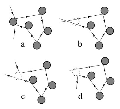
Figure 1: Four processes giving leading contribution to long-lived tail in velocity and spin correlation functions.

Indeed, one can see that the first term in Eq. (14) gives zero contribution to Eq. (13). Calculating the contribution of the second term we get

$$\delta\sigma(\theta,t)=-\frac{\sigma_{tr}^{2}}{4\pi^{2}v}\frac{\cos\theta}{t^{2}}.$$ (15)

It worth noting that $\delta\sigma(\theta,t)dt$ has a dimension of length and can be interpreted as a correction to the scattering cross-section due to diffusive returns taking the time lying in the interval $[t,t+dt].$

The diffusion equation can be obtained by standard means from kinetic equation (9) with the use of Eq. (7). As a result we find the diffusion-like equation for the isotropic part of the spin density $s_{0}=\langle s(\mathbf{p},\mathbf{r},t)\rangle_{\theta}$ (averaging is taken over momentum directions):

$$\frac{\partial\mathbf{s}_{0}}{\partial t}=D\tilde{\Delta}\left(\mathbf{s}_{0}-\frac{n\sigma_{tr}^{2}\tau}{4\pi}\int_{\tau}^{\infty}\frac{\mathbf{s}_{0}(t-t^{\prime})dt^{\prime}}{t^{\prime 2}}\right),$$ (16)

where $\tilde{\Delta}=\hat{T}(x)\Delta\hat{T}(x)^{-1}=(\partial/\partial x+q\hat{\epsilon})^{2}+\partial^{2}/\partial y^{2}$ and $\hat{\epsilon}$ is the antisymmetric tensor: $\hat{\epsilon}\mathbf{s}=[\mathbf{e}_{z}\times\mathbf{s}]$. Eq. (16) describes the spin dynamics in the diffusion approximation. It simplifies in the homogeneous case:

$$\frac{\partial\mathbf{s}_{0}}{\partial t}=-\frac{\mathbf{s}_{0}}{\tau_{S}}+\frac{n\sigma_{tr}^{2}\tau}{4\pi\tau_{S}}\int_{\tau}^{\infty}\frac{\mathbf{s}_{0}(t-t^{\prime})dt^{\prime}}{t^{\prime 2}}.$$ (17)

Here $1/\tau_{S}=Dq^{2}=(\alpha p_{F})^{2}\tau/2$ is the Dyakonov-Perel’ spin relaxation rate. The initial condition for (17) is $\mathbf{s}_{0}(0)=s_{\rm i}$ (we also assume that $\mathbf{s}_{0}(t)=0$ for $t<0$). Neglecting the second term in the rhs of Eq. (17) we get the exponential relaxation $\mathbf{s}_{0}(t)=\exp(-t/\tau_{S})\mathbf{s}_{\rm i}$ perel . This solution is valid until $\exp(-t/\tau_{S})\sim n\sigma^{2}_{tr}\tau\tau_{S}/t^{2}.$ For larger times, $\int^{t}_{\tau}dt^{\prime}\mathbf{s}_{0}(t-t^{\prime})/t^{\prime 2}\approx\mathbf{s}_{\rm i}\tau_{S}/t^{2}$ and one can neglect the term $\partial\mathbf{s}_{0}/\partial t$ in Eq. (17). As a result we find that the polarization has a long-lived tail

$$\mathbf{s}_{0}(t)\approx\frac{n\sigma_{tr}^{2}\tau\tau_{S}}{4\pi t^{2}}\mathbf{s}_{\rm i}=\frac{\sigma_{tr}}{l}\frac{\tau\tau_{S}}{4\pi t^{2}}\mathbf{s}_{\rm i},$$ (18)

which is positive in contrast to Eq. (1).

Eq. (18) was derived for the case of strong scatterers with low concentration ($nd^{2}\ll 1$). The opposite limiting case (weak scatterers, $nd^{2}\gg 1$) corresponds to the smooth random potential with the correlation function $\langle U(\mathbf{r})U(\mathbf{r}^{\prime})\rangle=\int\kappa_{q}\exp[i\mathbf{q}(\mathbf{r}-\mathbf{r}^{\prime})]d^{2}\mathbf{q}/(2\pi)^{2}$. In this case, the collision integral can be written as a sum of the Boltzmann collision integral $\hat{J}_{B}=(1/\tau)(\partial^{2}/\partial\varphi^{2})$ and

$$\hat{J}^{*}=\frac{\partial}{\partial\varphi}\left[\int_{0}^{\infty}dt[\mathbf{n}\times\mathbf{f}(\mathbf{r})][\mathbf{n}\times\mathbf{f}(\mathbf{r}-\mathbf{v}t)]-\frac{1}{\tau}\right]\frac{\partial}{\partial\varphi},$$ (19)

where $1/\tau=(1/2\pi m^{2}v_{F}^{3})\int_{0}^{\infty}q^{2}\kappa_{q}dq$ and $\mathbf{f}=-\nabla U(\mathbf{r})/mv_{F}$ d/dr . One can check that $\langle\hat{J}^{*}\rangle=0.$ Substituting Eq. (19) into Eq. (10), using Eq. (14) and accounting for two types of correlations pol we get

$$\delta\hat{J}\mathbf{s}(\varphi)=\frac{2\pi^{2}d^{2}}{\tau^{2}}\int_{0}^{\infty}dt^{\prime}[G^{\prime\prime}(0,t^{\prime})\frac{\partial^{2}\mathbf{s}(\varphi,t-t^{\prime})}{\partial\varphi^{2}}~{}+$$

$$G^{\prime\prime}(\pi,t^{\prime})\frac{\partial^{2}\mathbf{s}(\varphi+\pi,t-t^{\prime})}{\partial\varphi^{2}}],$$ (20)

where $G^{\prime\prime}(\varphi,t)=\partial^{2}G(0,\varphi,t)/\partial\varphi^{2}.$ The calculations analogous to the case of strong scattering centers yield

$$\mathbf{s}_{0}(t)=\frac{d^{2}}{l^{2}}\frac{\tau\tau_{S}}{t^{2}}~{}\mathbf{s}_{\rm i}.$$ (21)

In Eqs. (20) and (21), $d=\sqrt{2\int_{0}^{\infty}\kappa_{q}^{2}q^{3}dq}/\int_{0}^{\infty}\kappa_{q}q^{2}dq.$

Above we assumed that $\mathbf{s}_{\rm i}$ is homogenous. For slowly varying $\mathbf{s}_{\rm i}(\mathbf{r}),$ the derived equations relate $\mathbf{s}_{0}(\mathbf{r},t)$ with $\mathbf{s}_{\rm i}(\mathbf{r})$ provided that the spatial scale of inhomogeneity $L$ is large compared to $\sqrt{D\tau_{S}}\sim 1/m\alpha$ D/G . One can show that in the opposite case $l\ll L\ll 1/m\alpha,$ these equations are also valid relating $\int d\mathbf{r}~{}\mathbf{s}_{0}(\mathbf{r},t)$ with $\int d\mathbf{r}~{}\mathbf{s}_{\rm i}(\mathbf{r}).$

Let us briefly discuss the role of electron-electron interaction. Such interaction manifests itself both in inelastic scattering and in the additional, with respect to the diffusion process, decay of density fluctuation due to Maxwell relaxation. Such a relaxation partially suppresses the long-lived tail in velocity correlation function (1) leading to the faster decay ufn : $1/t^{2}\to r^{2}_{B}/Dt^{3},$ where $r_{B}$ is the 2D screening length, which coincides with the Bohr radius. In contrast to this, the Maxwell relaxation has no effect on the spin dynamics because in the classical approximation the spin fluctuations are not coupled to the charge fluctuations and, as a consequence, do not lead to creation of long-range electrical field responsible for Maxwell relaxation.

As for electron-electron collisions, their characteristic time $\tau_{ee}$ is inversely proportional to $T^{2}.$ For relatively small temperatures, $\tau_{ee}\gg\tau$ and electron-electron collisions do not have any effect on the spin relaxation in the classical approximation. In the opposite limiting case, $\tau_{ee}\ll\tau,$ electron-electron collisions might suppress spin relaxation glazov . The detailed discussion of this case is out of the scope of this paper. We believe that $1/t^{2}$ dependence of long-time polarization is also valid for this case, while the coefficient in this dependence might change.

Finally, we compare non-Markovian tail in the spin polarization (Eqs. (18), (21)) with the long-lived tail induced by weak localization my1 : $\mathbf{s}_{0}(t)=\mathbf{s}_{\rm i}(\tau_{S}/\pi k_{F}lt)\exp(-t/\tau_{\varphi}),$ where $\tau_{\varphi}$ is the phase-breaking time. At $T=0,$ when $\tau_{\varphi}=\infty,$ long-time spin dynamics is determined by weak localization. However, for $T\neq 0$ classical memory effects dominate at $t\gg\tau_{\varphi}.$

In conclusion, we developed a theory of long-time spin dynamics for 2D system, where spin-orbit-induced magnetic field is parallel to a fixed axis. We showed that independently on the type of disorder the non-equilibrium spin polarization in such a system decays as $1/t^{2}$ (for $t\to\infty$) due to purely classical memory effects.

- (1)
- (2) M. Fogler et al., Phys. Rev. B 56, 6823 (1997);
- (3) E.M. Baskin and M.V. Entin, Physica B 249 , 805 (1998).
- (4) A.V. Bobylev et al., J. Stat. Phys. 87, 1205 (1997).
- (5) A.D. Mirlin et al., Phys. Rev. Lett. 87, 126805 (2001); D.G. Polyakov et al., Phys. Rev. B 64, 205306 (2001).
- (6) A. Dmitriev, M. Dyakonov, R. Jullien, Phys. Rev. B 64, 233321 (2001).
- (7) A.D. Mirlin et al., Phys. Rev. Lett. 83, 2801 (1999).
- (8) A.P. Dmitriev, M. Dyakonov, R. Jullien, Phys. Rev. Lett. 89, 266804 (2002).
- (9) V.V. Cheianov, A.P. Dmitriev, V.Yu. Kachorovskii, Phys. Rev. B 68, 201304 (2003); Phys. Rev. B 70, 245307 (2004).
- (10) J. Wilke et al., Phys. Rev. B 61, 13774 (2000)
- (11) D.G. Polyakov, F. Evers and I.V. Gornyi, Phys. Rev. B 65, 125326 (2002).
- (12) M.H. Ernst and A. Weyland, Phys. Lett. 34 A, 39 (1971).
- (13) E.H. Hauge, in Transport Phenomena, edited by G. Kirczenow and J. Marro, Lecture Notes in Physics, Vol. 31 (Springer, Berlin, 1974), p. 337.
- (14) A. Dmitriev, M. Dyakonov, and R. Jullien, Phys. Rev. B 71, 155333 (2005).
- (15) Semiconductor Spintronics and Quantum Computation, eds. D.D. Awschalom, D. Loss, and N. Samarth (Springer-Verlag, Berlin, 2002).
- (16) M.I. Dyakonov and V.I. Perel’, Sov. Phys. Solid State 13, 3023 (1972).
- (17) A.G. Mal’shukov, K.A. Chao and M. Willander, Phys. Rev. B 52, 5233 (1995); Phys. Rev. Lett. 76, 3794 (1996).
- (18) I.S. Lyubinskiy, V.Yu. Kachorovskii, Phys. Rev. B 70, 205335 (2004); Phys. Rev. Lett 94, 076406 (2005).
- (19) M.I. Dyakonov and V.Yu. Kachorovskii, Sov. Phys. Semicond. 20, 110 (1986).
- (20) Y. Ohno et al., Phys. Rev. Lett. 83, 4196 (1999).
- (21) T. Adachi et al., Physica E (Amsterdam) 10, 36 (2001).
- (22) W.H. Lau and M.E. Flatté, J. Appl. Phys. 91, 8682 (2002).
- (23) O.Z. Karimov et al., Phys. Rev. Lett. 91, 246601 (2003).
- (24) K.C. Hall et al., Phys. Rev. B 68, 115311 (2003).
- (25) S. Döhrmann et al., Phys. Rev. Lett. 93, 147405 (2004).
- (26) G. Dresselhaus, Phys. Rev. 100, 580 (1955).
- (27) Yu. Bychkov and E. Rashba, JETP Lett. 39, 78 (1984).
- (28) F.G. Pikus and G.E. Pikus, Phys. Rev. B 51, 16928 (1995)
- (29) N.S. Averkiev and L.E. Golub, Phys. Rev. B 60, 15582 (1999)
- (30) A.A. Kisilev and K.W. Kim, Phys. Status Solidi (b) 221, 491 (2000)
- (31) J. Schliemann, J.C. Egues, and D. Loss, Phys. Rev. Lett. 90, 146801 (2003).
- (32) J. Schliemann and D. Loss, Phys. Rev. B 68, 165311 (2003).
- (33) J. Nitta et al., Phys. Rev. Lett. 78, 1335 (1997).
- (34) V.I. Kozub, Sov. Phys. Solid State, 26, 1186 (1984); Yu.M. Gal’perin and V.I. Kozub, Sov. Phys. JETP, 73, 179 (1991).
- (35) L.S. Levitov and E.I. Rashba, Phys. Rev. B, 67, 115324 (2003).
- (36) In a purely classical case (with an exception for Lorentz gas model) due to divergent contribution of small-angle scattering. However, our final result only depends on (see Eq. (15)) thus justifying the approach based on classical consideration.
- (37) Actually, collision integral also contains terms with spatial derivatives. However, they give negligible contribution to velocity and spin correlation functions.
- (38) Note that is a characteristic scale of non-decaying spin oscillations which might exist in the system under discussion (see Ref. loss1 ).
- (39) F. Evers et al., Usp. Fiz. Nauk (Suppl.) 171, 27 (2001)
- (40) M.M. Glazov and E.L. Ivchenko, JETP Lett. 75, 403 (2002).