Orbital and spin physics in LiNiO₂ and NaNiO₂

Abstract

We derive a spin-orbital Hamiltonian for a triangular lattice of $e_{g}$ orbital degenerate (Ni³⁺) transition metal ions interacting via 90^∘ superexchange involving (O^2-) anions, taking into account the on-site Coulomb interactions on both the anions and the transition metal ions. The derived interactions in the spin-orbital model are strongly frustrated, with the strongest orbital interactions selecting different orbitals for pairs of Ni ions along the three different lattice directions. In the orbital ordered phase, favoured in mean field theory, the spin-orbital interaction can play an important role by breaking the $U(1)$ symmetry generated by the much stronger orbital interaction and restoring the threefold symmetry of the lattice. As a result the effective magnetic exchange is non-uniform and includes both ferromagnetic and antiferromagnetic spin interactions. Since ferromagnetic interactions still dominate, this offers yet insufficient explanation for the absence of magnetic order and the low-temperature behaviour of the magnetic susceptibility of stoichiometric LiNiO₂. The scenario proposed to explain the observed difference in the physical properties of LiNiO₂ and NaNiO₂ includes small covalency of Ni–O–Li–O–Ni bonds inducing weaker interplane superexchange in LiNiO₂, insufficient to stabilize orbital long-range order in the presence of stronger intraplane competition between superexchange and Jahn-Teller coupling.

1 Introduction

The low-temperature magnetic behaviour of LiNiO₂ has remained puzzling ever since its peculiar properties were discovered [1]. For no apparent reason, LiNiO₂ does not show magnetic order nor a cooperative Jahn-Teller effect down to the lowest temperatures, which is very different from the conventional behaviour observed in its sister compound NaNiO₂.

Structurally the two systems represent an interesting special category within the class of correlated transition metal (TM) oxides. LiNiO₂ has a layered structure [see figure 1(a)]: it is rhombohedral, consisting of successive (111) planes occupied by Li⁺, O^2-, Ni³⁺, and O^2- ions. Thus the Ni³⁺ ions are on a triangular lattice, with each direct Ni–Ni bond lying along the diagonal of a nearly square Ni–O–Ni–O plaquette, the Ni–O–Ni bonds being close to 90 degrees. This is distinct from the more commonly encountered situation where the bond between two transition metal ions through the ligand ion connecting them is close to linear (180 degrees), as e.g. in the perovskites. As pointed out by Mostovoy and Khomskii [2], this difference should have important consequences for the orbital and magnetic superexchange (SE) in LiNiO₂, since the SE within a Ni plane with Ni${}^{3+}(t_{2g}^{6}e_{g}^{1})$ ions would originate predominantly from virtual charge transfer excitations $e^{1}2p^{6}e^{1}\rightleftharpoons e^{2}2p^{5}e^{1}\rightleftharpoons e^{2}2p^{4}e^{2}$ along the 90 degrees Ni–O–Ni bonds.

Over the years, a number of experiments (magnetic susceptibility, ESR, NMR, neutron scattering) have been performed on LiNiO₂ samples of varying stoichiometry [3]–[11]. From these data one has concluded that the presence of excess Ni ions in the lithium layers introduces extra ferromagnetic (FM) coupling between the nickel layers. In addition, for the samples closest to perfect stoichiometry a positive Curie-Weiss temperature was found, indicating that the in-plane exchange is also FM. This is not in accordance with the description given initially by Hirakawa et al[3], namely that LiNiO₂ would be a triangular lattice antiferromagnet (TALAF). Actually, this assumption was the original motivation for performing magnetic measurements on LiNiO₂, since the TALAF for spin $S=1/2$ is a frustrated system and the ground state might be some kind of quantum liquid [12] instead of the classical 120^∘ rotated spin arrangement.

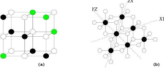
Figure 1: Structure of LiNiO₂: (a) Fragment of 3D crystal structure, with Ni ions shown by filled circles, Li ions by gray circles, and O ions by open circles. (b) Nickel layer with adjacent oxygen layers. Each Ni³⁺ ion (black circles) is surrounded by six oxygens (open circles). The directions of the Ni$-$Ni bonds are labelled as $XY$, $YZ$ and $ZX$, corresponding in each case to the plane spanned by the connecting Ni$-$O bonds.

At first sight the FM nature of the in-plane correlations is not surprising when one looks at the three-dimensional (3D) crystal structure (figure 1). As the neighbouring Ni³⁺ ions are connected via two Ni-O-Ni bridges, one has the case of 90^∘ SE, which the classical Goodenough-Kanamori-Anderson rules [13] apparently predict to be FM. In a strong crystal field the ground state of Ni³⁺ is the low-spin ($t_{2g}^{6}e_{g}^{1}$) configuration, so that direct exchange between $t_{2g}$ electrons does not occur. The exchange interactions between different nickel layers should also be FM [14], so that one naively expects a long-range ordered FM ground state. However, for LiNiO₂ no long-range magnetic order was found down to temperatures very close to $0$ K and the magnetic susceptibility gradually diverges, giving the impression that the FM correlations mysteriously disappear. A suggestion was made by Feiner, Oleś and Zaanen [15] that the $e_{g}$ orbital degeneracy of the Ni³⁺ ion and partly antiferromagnetic (AF) interactions might be responsible for this peculiar behaviour.

The issue was then addressed by Mostovoy and Khomskii (MK) in an important paper [2] in which they proposed a realistic spin-and-orbital model for the Ni plane, which includes the Coulomb repulsion and the Hund’s rule exchange splitting on oxygen. They arrived at the conclusion that there is a huge degeneracy in the orbital sector, which is not resolved at the mean-field (MF) level. Yet orbital order is favoured over an orbital liquid state by the order-out-of-disorder mechanism, while they claimed that anyway the magnetic interaction is always FM [2]. From the absence of an orbital ordered state in LiNiO₂ they concluded that the difference between LiNiO₂ and NaNiO₂ is probably extrinsic, due to disorder or electron-lattice interaction. Apparently this has now become the predominant view, and is as yet not inconsistent with experiments.

However, a conclusion concerning the nature of the magnetic interactions and the origin of the peculiar properties of LiNiO₂ had better be drawn only after the theoretical prediction for the intrinsic in-plane behaviour is fully established. We believe that this is not the case and therefore reanalyze the situation in this paper. Our finding is that upon inclusion of the Hund’s rule splitting also on the Ni ions and correction of what is apparently a mistake in the MK analysis, both FM and AF interactions can occur in the Ni plane, depending upon the orbital arrangement. Admittedly, this still leaves the difference between LiNiO₂ and NaNiO₂ to be explained, but it reopens the case for an intrinsic mechanism since different orbital phases in the Ni plane could give rise to different magnetic interactions.

The paper is organized as follows. In section 2 we present the notation used in the following sections for the spin and orbital operators used to derive the microscopic model. In section 3 we review some issues concerning SE, in particular with regard to the Ni–O–Ni 90^∘ bond, and compare this case with the standard situation encountered for 180^∘ bonds in TM perovskites. The spin-orbital SE model for the triangular Ni planes of LiNiO₂ and NaNiO₂ is presented in section 4. Next we discuss the strong frustration of the orbital and spin interactions in this model, and we investigate its consequences and present possible ground states, obtained using MF theory for a pair of Ni ions (section 5) and for the entire plane (section 6). The implications of the model for the physical properties of LiNiO₂ and NaNiO₂ are discussed in section 7. Finally, in section 8 the main conclusions and a summary are given. Technical details of the derivation of the model are presented in A.

2 Pseudospin formalism for degenerate $e_{g}$ orbitals

For the twofold degenerate $e_{g}$ orbital state at each site local operators corresponding to pseudospin $T=1/2$ are introduced, i.e. $T_{i}^{x}$, $T_{i}^{y}$ and $T_{i}^{z}$, acting as half the Pauli matrices $\sigma^{x},\sigma^{y}$ and $\sigma^{z}$ on the two-dimensional (2D) orbital Hilbert space at site $i$ with basis

$${1\choose 0}_{i}\,\equiv|iz\rangle\,\equiv d_{i,3z^{2}-r^{2}}^{\dagger}|0\rangle,\hskip 56.9055pt\displaystyle{0\choose 1}_{i}\,\equiv|i\bar{z}\rangle\,\equiv d_{i,x^{2}-y^{2}}^{\dagger}|0\rangle.$$ (1)

A general superposition is given by

$$|i\theta_{i}\rangle=\cos(\theta_{i}/2)\,\,\displaystyle{1\choose 0}_{i}+\sin(\theta_{i}/2)\,\,\displaystyle{0\choose 1}_{i},$$ (2)

which for example at $\theta_{i}=\frac{\pi}{3}$ corresponds to a $d_{z^{2}-x^{2}}$ orbital. The expectation values of the pseudospin operators in the general orbital state (2) are

$$\langle T_{i}^{z}\rangle={\textstyle\frac{1}{2}}\cos\theta_{i},\hskip 28.45274pt\langle T_{i}^{x}\rangle={\textstyle\frac{1}{2}}\sin\theta_{i},\hskip 28.45274pt\langle T_{i}^{y}\rangle=0.$$ (3)

In order to make the formalism more flexible and to include explicitly the cubic symmetry of the $e_{g}$ orbitals, it is convenient to define two more equivalent basis sets by

$$|i\alpha\rangle\equiv d_{i,3\alpha^{2}-r^{2}}^{\dagger}|0\rangle,\hskip 28.45274pt\qquad \left(\{\alpha,\beta,\gamma\}\;\;\textrm{a cyclic}\right.$$

$$|i\bar{\alpha}\rangle\equiv d_{i,\beta^{2}-\gamma^{2}}^{\dagger}|0\rangle, \left.\;\;\textrm{permutation of\/}\;\;\{x,y,z\}\right)$$ (4)

and corresponding rotated pseudospin operators $I_{i}^{\alpha}$ and $\bar{I}_{i}^{\alpha}$ behaving like $T_{i}^{z}$ and $T_{i}^{x}$ with respect to those basis sets, i.e.

$$I_{i}^{x}=-{\textstyle\frac{1}{2}}T_{i}^{z}-{\textstyle\frac{\sqrt{3}}{2}}T_{i}^{x},\hskip 56.9055pt \bar{I}_{i}^{x}=+{\textstyle\frac{\sqrt{3}}{2}}T_{i}^{z}-{\textstyle\frac{1}{2}}T_{i}^{x},$$

$$I_{i}^{y}=-{\textstyle\frac{1}{2}}T_{i}^{z}+{\textstyle\frac{\sqrt{3}}{2}}T_{i}^{x}, \bar{I}_{i}^{y}=-{\textstyle\frac{\sqrt{3}}{2}}T_{i}^{z}-{\textstyle\frac{1}{2}}T_{i}^{x},$$

$$I_{i}^{z}=T_{i}^{z}, \bar{I}_{i}^{z}=T_{i}^{x},$$ (5)

which satisfy the identities

$$I_{i}^{x}+I_{i}^{y}+I_{i}^{z}=0,\hskip 56.9055pt\bar{I}_{i}^{x}+\bar{I}_{i}^{y}+\bar{I}_{i}^{z}=0.$$ (6)

We can now introduce on-site orbital projection operators by

$${\mathcal{P}}_{i}^{\alpha}=({\textstyle\frac{1}{2}}{\bi I}_{i}+I_{i}^{\alpha}),\hskip 56.9055pt{\mathcal{P}}_{i}^{\bar{\alpha}}=({\textstyle\frac{1}{2}}{\bi I}_{i}-I_{i}^{\alpha}),$$ (7)

where ${\bi I}_{i}$ is the unit operator in the 2D orbital Hilbert space at site $i$.

We further define two sets of (mutually dependent) orbital-pair operators, $\{{\mathcal{I}}_{ij}^{\alpha\beta},{\mathcal{J}}_{ij}^{\alpha\beta}\}$ and $\{{\mathcal{V}}_{ij}^{\alpha\beta},{\mathcal{W}}_{ij}^{\alpha\beta}\}$, all of which refer to a pair of nearest neighbour TM ions with their bond $\langle ij\rangle$ lying in the $\alpha\beta$ plane (see figure 1(b)),

$${\mathcal{I}}_{ij}^{\alpha\beta} = ({\bi I}_{i}+{\mathcal{P}}_{i}^{\bar{\alpha}})({\bi I}_{j}+{\mathcal{P}}_{j}^{\bar{\beta}})+({\bi I}_{i}+{\mathcal{P}}_{i}^{\bar{\beta}})({\bi I}_{j}+{\mathcal{P}}_{j}^{\bar{\alpha}})$$ (8)

$$= ({\textstyle\frac{3}{2}}{\bi I}_{i}-I_{i}^{\alpha})({\textstyle\frac{3}{2}}{\bi I}_{j}-I_{j}^{\beta})+({\textstyle\frac{3}{2}}{\bi I}_{i}-I_{i}^{\beta})({\textstyle\frac{3}{2}}{\bi I}_{j}-I_{j}^{\alpha}),$$

$${\mathcal{J}}_{ij}^{\alpha\beta} = ({\bi I}_{i}-{\mathcal{P}}_{i}^{\bar{\alpha}})({\bi I}_{j}-{\mathcal{P}}_{j}^{\bar{\beta}})+({\bi I}_{i}-{\mathcal{P}}_{i}^{\bar{\beta}})({\bi I}_{j}-{\mathcal{P}}_{j}^{\bar{\alpha}})$$ (9)

$$= ({\textstyle\frac{1}{2}}{\bi I}_{i}+I_{i}^{\alpha})({\textstyle\frac{1}{2}}{\bi I}_{j}+I_{j}^{\beta})+({\textstyle\frac{1}{2}}{\bi I}_{i}+I_{i}^{\beta})({\textstyle\frac{1}{2}}{\bi I}_{j}+I_{j}^{\alpha}),$$

$${\mathcal{V}}_{ij}^{\alpha\beta} = -{\bi I}_{i}\,(I_{j}^{\alpha}+I_{j}^{\beta})-(I_{i}^{\alpha}+I_{i}^{\beta})\,{\bi I}_{j}={\bi I}_{i}\,I_{j}^{\gamma}+I_{i}^{\gamma}\,{\bi I}_{j},$$ (10)

$${\mathcal{W}}_{ij}^{\alpha\beta} = 2\,(I_{i}^{\alpha}\,I_{j}^{\beta}+I_{i}^{\beta}\,I_{j}^{\alpha})=2\,(I_{i}^{\gamma}\,I_{j}^{\gamma}-I_{i}^{\alpha}\,I_{j}^{\alpha}-I_{i}^{\beta}\,I_{j}^{\beta}).$$ (11)

Their expectation values in a pair state $|i\theta_{i}\rangle|j\theta_{j}\rangle$ are given by

$$\langle{\mathcal{I}}_{ij}^{\alpha\beta}\rangle = {\textstyle\frac{1}{8}}[35+12\cos(\theta_{+}+\chi_{\gamma})\,\cos\theta_{-}+4\cos^{2}(\theta_{+}+\chi_{\gamma})-2\cos^{2}\theta_{-}],$$ (12)

$$\langle{\mathcal{J}}_{ij}^{\alpha\beta}\rangle = {\textstyle\frac{1}{8}}[3-4\cos(\theta_{+}+\chi_{\gamma})\,\cos\theta_{-}+4\cos^{2}(\theta_{+}+\chi_{\gamma})-2\cos^{2}\theta_{-}],$$ (13)

$$\langle{\mathcal{V}}_{ij}^{\alpha\beta}\rangle = \cos(\theta_{+}+\chi_{\gamma})\,\cos\theta_{-},$$ (14)

$$\langle{\mathcal{W}}_{ij}^{\alpha\beta}\rangle = {\textstyle\frac{1}{4}}[4\cos^{2}(\theta_{+}+\chi_{\gamma})-2\cos^{2}\theta_{-}-1]={\textstyle\frac{1}{4}}[2\cos(2\theta_{+}+2\chi_{\gamma})-\cos 2\theta_{-}],$$ (15)

where $\theta_{\pm}=(\theta_{i}\pm\theta_{j})/2$, and $\chi_{x}={\textstyle\frac{2\pi}{3}}$, $\chi_{y}=-{\textstyle\frac{2\pi}{3}}$, $\chi_{z}=0$.

Finally we introduce bond projection operators, needed for specifying the SE interactions between a pair of TM ions. For the spin part we will use the familiar projection operators for spin triplet and spin singlet,

$${\bi Q}^{T}_{ij}={\textstyle\frac{3}{4}}{\bf 1}_{ij}+{\bi S}_{i}\cdot{\bi S}_{j},\hskip 56.9055pt{\bi Q}^{S}_{ij}={\textstyle\frac{1}{4}}{\bf 1}_{ij}-{\bi S}_{i}\cdot{\bi S}_{j},$$ (16)

where ${\bf 1}_{ij}$ is the unit operator in the four-dimensional (4D) spin Hilbert space on the bond $\langle ij\rangle$. For the orbital part we will make use of

$${\mathcal{Q}}_{{\rm O},ij}^{\alpha\beta} = {\mathcal{P}}_{i}^{\alpha}{\mathcal{P}}_{j}^{\beta}+{\mathcal{P}}_{i}^{\beta}{\mathcal{P}}_{j}^{\alpha},$$ (17)

$${\mathcal{Q}}_{{\rm M},ij}^{\alpha\beta} = {\mathcal{P}}_{i}^{\alpha}{\mathcal{P}}_{j}^{\bar{\beta}}+{\mathcal{P}}_{i}^{\bar{\alpha}}{\mathcal{P}}_{j}^{\beta}+{\mathcal{P}}_{i}^{\beta}{\mathcal{P}}_{j}^{\bar{\alpha}}+{\mathcal{P}}_{i}^{\bar{\beta}}{\mathcal{P}}_{j}^{\alpha},$$ (18)

$${\mathcal{Q}}_{{\rm N},ij}^{\alpha\beta} = {\mathcal{P}}_{i}^{\bar{\alpha}}{\mathcal{P}}_{j}^{\bar{\beta}}+{\mathcal{P}}_{i}^{\bar{\beta}}{\mathcal{P}}_{j}^{\bar{\alpha}},$$ (19)

where the labelling will be explained in section 4. They are conveniently expanded in terms of the operators defined above, according to (with indices omitted for clarity)

$$\begin{array}[]{rcrcrcrcrcrcrl}{\mathcal{Q}}_{\rm O}&=&&&&&{\mathcal{J}}&=&{\textstyle\frac{1}{2}}{\bi I}&-&{\textstyle\frac{1}{2}}{\mathcal{V}}&+&{\textstyle\frac{1}{2}}{\mathcal{W}}&\\ {\mathcal{Q}}_{\rm M}&=&4{\bi I}&-&{\textstyle\frac{1}{2}}{\mathcal{I}}&-&{\textstyle\frac{3}{2}}{\mathcal{J}}&=&{\bi I}&&&-&{\mathcal{W}}&\\ {\mathcal{Q}}_{\rm N}&=&-2{\bi I}&+&{\textstyle\frac{1}{2}}{\mathcal{I}}&+&{\textstyle\frac{1}{2}}{\mathcal{J}}&=&{\textstyle\frac{1}{2}}{\bi I}&+&{\textstyle\frac{1}{2}}{\mathcal{V}}&+&{\textstyle\frac{1}{2}}{\mathcal{W}}&\!\!,\end{array}$$ (20)

where ${\bi I}\equiv{\bi I}_{ij}$ now denotes the identity in the 4D orbital-pair Hilbert space.

3 Superexchange for degenerate $e_{g}$ orbitals

If degenerate $e_{g}$ orbitals are partly filled, a spin-orbital Hamiltonian can be constructed from a degenerate-band Hubbard model in much the same way as one derives the AF Heisenberg model from the single-band Hubbard model at half-filling. The Hamiltonian of the $e_{g}$-band Hubbard model consists of two parts: there is a hopping term ${\mathcal{T}}$ modelling transfer of electrons between nearest-neighbour transition metal sites and a Hubbard (or Coulomb) term ${\mathcal{U}}$ describing the on-site interactions. In the situation where the number of sites equals the number of electrons, the ground state for ${\mathcal{T}}=0$ has twofold spin and twofold orbital degeneracy on each site. When we allow for a nonzero ${\mathcal{T}}$ as a small perturbation, the 4^N-fold degeneracy is lifted by virtual electron hopping involving excited states, and the effective Hamiltonian in second order perturbation theory is

$${\mathcal{H}}_{\rm eff}=\sum_{n\in\!\!\!/\,{\rm G}}{\mathcal{P}}_{\rm G}\,\Big{[}{\mathcal{T}}|n\rangle\frac{1}{E_{\rm G}-E_{n}}\langle n|{\mathcal{T}}\Big{]}\,{\mathcal{P}}_{\rm G},$$ (21)

where ${\mathcal{P}}_{\rm G}$ is a projection operator onto the ground state manifold of ${\mathcal{U}}$. The spin-orbital Hamiltonian is obtained by writing out (21) in terms of spin and orbital projection operators at each site $i$.

For a cubic lattice, such as in the perovskites KCuF₃ and K₂CuF₄, one can describe by this approach also the 180^∘ SE, thus treating it formally as direct exchange. The hopping term is taken as

$${\mathcal{T}}=-\bar{t}\sum_{\alpha}\,\sum_{\langle ij\rangle\parallel\alpha}\,\sum_{\sigma}\;d_{i\alpha\sigma}^{\dagger}\>d_{j\alpha\sigma},$$ (22)

expressing that hopping is only allowed between nearest-neighbour directional orbitals $|\alpha\rangle\equiv d_{3\alpha^{2}-r^{2}}^{\dagger}|0\rangle$ oriented along the connecting $\alpha$ axis ($\alpha$ being $x$, $y$ or $z$). In the following we will therefore call the $\alpha$-orbitals ‘hopping’ orbitals – since electrons in these orbitals can hop and contribute to the kinetic energy, and similarly call ‘non-hopping’ orbitals the $\bar{\alpha}$-orbitals ($|\bar{\alpha}\rangle\equiv d_{\beta^{2}-\gamma^{2}}^{\dagger}|0\rangle$), orthogonal to the $\alpha$-orbital and oriented perpendicular to the bond. In a one-dimensional chain this situation leads to a characteristic competition between itinerant and localized phases [16].

The on-site interactions on a TM ion can be represented by [17]

$${\mathcal{U}}_{\rm TM} = U\sum_{i\lambda}n_{i\lambda\uparrow}n_{i\lambda\downarrow}+\Big{(}U-\frac{5}{2}J_{\rm H}\Big{)}\sum_{i,\lambda<\mu}n_{i\lambda}n_{i\mu}-2J_{\rm H}\sum_{i,\lambda<\mu}{\bi s}_{i\lambda}\cdot{\bi s}_{i\mu}$$ (23)

$$+ J_{\rm H}\sum_{i,\lambda<\mu}\Big{(}d^{\dagger}_{i\lambda\uparrow}d^{\dagger}_{i\lambda\downarrow}d_{i\mu\downarrow}d_{i\mu\uparrow}+d^{\dagger}_{i\mu\uparrow}d^{\dagger}_{i\mu\downarrow}d_{i\lambda\downarrow}d_{i\lambda\uparrow}\Big{)},$$

and are characterized by two parameters: the intraorbital Coulomb energy $U$ and the exchange energy $J_{\rm H}$. The interorbital terms in equation (23) describe electron interactions between pairs of orthogonal orbitals, i.e., in the present subspace of $e_{g}$ orbitals one has $\lambda,\mu\in\{\alpha,\bar{\alpha}\}$. The excited states, generated in the virtual $d-d$ transitions and relevant for SE, have two electrons on the same ion, and ${\mathcal{U}}$ contributes a Coulomb repulsion energy $U$. In the $\bar{t}\ll U$ limit one thus derives an effective low-energy spin-orbital Hamiltonian with coupling constant $J_{\rm SE}\propto\bar{t}^{\,2}/U$, in which spin and orbital degrees of freedom are interrelated. By taking also the Hund’s rule exchange $J_{\rm H}$ into account one removes the classical degeneracy of magnetically ordered phases [18]. The stable phase at low temperatures has long-range orbital order of a particular type of mixed orbitals, leading to AF interactions along the $c$-axis and FM interactions in the $(a,b)$-plane. This ordering was verified experimentally and has been shown to be stable with respect to quantum fluctuations for large $J_{\rm H}$ [19].

In a more realistic treatment of SE one takes into account explicitly that the hopping takes place via the ligand oxygen ion. The hopping term is then taken as

$${\mathcal{T}}=-t\sum_{\alpha}\,\sum_{\langle ij\rangle\parallel\alpha}\,\sum_{\sigma}\;\Big{(}d_{i\alpha\sigma}^{\dagger}\>p_{j\alpha\sigma}+p_{j\alpha\sigma}^{\dagger}\>d_{i\alpha\sigma}\Big{)},$$ (24)

and describes charge transfer with amplitude $t\equiv t_{\sigma}$ between the TM-orbital $d_{3\alpha^{2}-r^{2}}$ and the oxygen $\sigma$-type $p$-orbital $p_{\alpha}$, where again the orbitals are oriented along the connecting $\alpha$-axis. The on-site interaction on oxygen is given by

$${\mathcal{U}}_{\rm O} = U_{\rm O}\sum_{j\lambda}n_{j\lambda\uparrow}n_{j\lambda\downarrow}+\Big{(}U_{\rm O}-\frac{5}{2}J_{\rm O}\Big{)}\sum_{j,\lambda<\mu}n_{j\lambda}n_{j\mu}-2J_{\rm O}\sum_{j,\lambda<\mu}{\bi s}_{j\lambda}\cdot{\bi s}_{j\mu}$$ (25)

$$+ J_{\rm O}\sum_{j,\lambda<\mu}\Big{(}p^{\dagger}_{j\lambda\uparrow}p^{\dagger}_{j\lambda\downarrow}p_{j\mu\downarrow}p_{j\mu\uparrow}+p^{\dagger}_{j\mu\uparrow}p^{\dagger}_{j\mu\downarrow}p_{j\lambda\downarrow}p_{j\lambda\uparrow}\Big{)},$$

with intraorbital Coulomb energy $U_{\rm O}$ and exchange energy $J_{\rm O}$. Here the operators $n_{j\lambda\sigma}$, $n_{j\lambda}$ and ${\bi s}_{j\lambda}$ refer to an oxygen ion at site $j$. For two-hole excitations in the three $2p$ orbitals, as arises when the SE is derived (see below), this local problem and the excitation spectrum are isomorphic to those for three $t_{2g}$ orbitals filled by two electrons as in the vanadates [20]. The effective Hamiltonian is now obtained in fourth order perturbation theory,

$${\mathcal{H}}_{\rm eff}=\sum_{k,l,m\in\!\!\!/\,{\rm G}}{\mathcal{P}}_{\rm G}\Big{[}{\mathcal{T}}|k\rangle\frac{1}{E_{\rm G}-E_{k}}\langle k|{\mathcal{T}}|l\rangle\frac{1}{E_{\rm G}-E_{l}}\langle l|{\mathcal{T}}|m\rangle\frac{1}{E_{\rm G}-E_{m}}\langle m|{\mathcal{T}}\Big{]}{\mathcal{P}}_{\rm G}.$$ (26)

In the case of a 180^∘ TM–O–TM bond $\langle ij\rangle$ this is unproblematic. For the so-called $U$-term (Anderson or delocalization process) [13], where an electron is effectively transferred from one TM ion to the other TM ion, schematically represented as

$$e^{1}p^{6}e^{1}\rightarrow e^{1}p^{5}e^{2}\rightarrow e^{0}p^{6}e^{2}\rightarrow e^{1}p^{5}e^{2}\rightarrow e^{1}p^{6}e^{1},$$

one can simply replace $\bar{t}$ by $t_{\sigma}^{2}/\Delta$, where $\Delta$ is the excitation energy for transferring an electron from O to TM, and so the coupling constant in the effective Hamiltonian becomes

$$J_{U}\propto\frac{t_{\sigma}^{4}}{\Delta^{2}}\,\frac{1}{U}.$$ (27)

Note that the orbital filled in the second step is necessarily the same, also as regards spin, as the one emptied in the first step. The so-called $\Delta$-term (Goodenough process or correlation effect) [13] involves instead electron transfer of two electrons from the connecting oxygen ion, one to each of the TM neighbours,

$$e^{1}p^{6}e^{1}\,\rightarrow\,e^{1}p^{5}e^{2}\,\rightarrow\,e^{2}p^{4}e^{2}\rightarrow\,e^{1}p^{5}e^{2}\,\rightarrow\,e^{1}p^{6}e^{1}.$$

Here the oxygen $2p^{4}$ configuration involved has two holes with opposite spin on the same $\sigma$-type $p$-orbital, giving always the same intermediate state at the oxygen ion with energy $2\Delta+U_{\rm O}$, and the contributions to the effective Hamiltonian have coupling constant

$$J_{\Delta}\propto\frac{t_{\sigma}^{4}}{\Delta^{2}}\,\Big{(}\frac{1}{2\Delta+U_{\rm O}}-\frac{1}{2\Delta}\Big{)}=-\frac{t_{\sigma}^{4}}{\Delta^{2}}\,\frac{U_{\rm O}}{2\Delta(2\Delta+U_{\rm O})}.$$ (28)

The reason for the subtraction of the term $\propto 1/{2\Delta}$ will be discussed below. For a 180^∘ TM–O–TM bond the two processes (Anderson and Goodenough) make qualitatively similar contributions to the effective Hamiltonian (at least for a single $e_{g}$ electron on each TM ion [21]) because both involve $\sigma$-type hopping. As the terms contributed to ${\mathcal{H}}_{\rm eff}$ have identical form, they can be formally generated by the second-order formalism of direct exchange above, even though this models only the process giving the $U$-term in the SE. To obtain the coupling constants one can simply add equations (27) and (28). As these are generally of the same order of magnitude, inclusion of the $\Delta$-term is important quantitatively, and is essential to describe the trend in the strength of SE within the $3d$ TM series [22, 23].

In the case of a 90^∘ TM–O–TM bond, as on a triangular lattice, the situation is very different. In the $U$-term (Anderson) process the oxygen orbital through which the electron is being transferred is now $\sigma$-type for one TM ion but $\pi$-type for the other one. Therefore this process can only occur if it involves a (deep-lying) $t_{2g}$ orbital,

$$(t_{2}^{6}e^{1})p^{6}(t_{2}^{6}e^{1})\,\leftrightarrow\,(t_{2}^{6}e^{1})p^{5}(t_{2}^{6}e^{2})\,\leftrightarrow\,(t_{2}^{5}e^{1})p^{6}(t_{2}^{6}e^{2}),$$

and thus contributes to the effective Hamiltonian a term with coupling constant

$$J_{U}\propto\frac{t_{\sigma}^{2}t_{\pi}^{2}}{\Delta^{2}}\,\frac{1}{U+\Delta_{\rm CF}},$$ (29)

since the energy of the middle intermediate state is increased by the crystal field splitting $\Delta_{\rm CF}$, and the hopping parameter for the $t_{2g}$ orbital is $t_{\pi}$ instead of $t_{\sigma}$. In the charge transfer terms ($\Delta$ process) the oxygen $2p^{4}$ states now involve two holes on different $p$-orbitals, each of ${\sigma}$-type but with respect to a different TM neighbour. This implies that the oxygen Coulomb interaction involved is now the interorbital interaction $U_{\rm O}^{\prime}\equiv U_{p}$ instead of the intraorbital interaction $U_{\rm O}=U_{\rm O}^{\prime}+2J_{p}$. Moreover it leads to a singlet-triplet splitting, with energies $U_{s}=U_{p}+J_{p}$ and $U_{t}=U_{p}-J_{p}$, where $J_{p}\equiv J_{\rm O}$ is the (Hund’s rule) exchange on oxygen, and thus the contributions to the effective Hamiltonian have coupling constants

$$J_{\Delta}^{\pm}\propto\frac{t_{\sigma}^{4}}{\Delta^{2}}\,\Big{(}\frac{1}{2\Delta+U_{p}\pm J_{p}}-\frac{1}{2\Delta}\Big{)}=-\frac{t_{\sigma}^{4}}{\Delta^{2}}\,\frac{U_{p}\pm J_{p}}{2\Delta(2\Delta+U_{p}\pm J_{p})}.$$ (30)

From equations (29) and (30) one observes that the dominant contribution to the SE comes from the $\Delta$-term (Goodenough process), since $t_{\sigma}^{2}/t_{\pi}^{2}\simeq 4$ [24], while $U+\Delta_{\rm CF}\gg 2\Delta$ and $U_{p}\simeq 2\Delta$ [25, 26, 27]. This was already pointed out in reference [13], as well as the fact that the magnetic interaction should then be FM, as equation (30) shows, which is one of the famous Goodenough-Kanamori-Anderson rules. Nevertheless, one should be careful not to jump to conclusions here, since the implications of the orbital SE interaction were not fully considered by Goodenough [13] (the case explicitly considered was the SE between Ni²⁺ ($t_{2g}^{6}e_{g}^{2}$ : ${}^{3}\!A_{2}$) ions [28], where the two $e_{g}$ orbitals are both occupied by one electron, and no orbital effects can arise). It is further clear that the dominant $\Delta$-term (Goodenough contribution) cannot be represented well as an effective second order direct exchange. Yet this was attempted in a recent paper [29]: this has the merit of deriving the most general form of the effective Hamiltonian purely based on symmetry considerations, but it cannot capture the dependence on the most relevant parameters $U_{p}$ and $J_{p}$ (actually only the weaker $U$-term SE, dependent upon the splitting of the intermediate Ni²⁺ configurations, is being described).

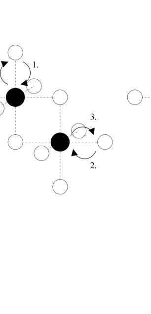
Figure 2: Double charge transfer excitations in LiNiO₂: (a) Isolated excitations which renormalize the electronic structure, and (b) Joined excitations involving a common oxygen site, which contribute to the superexchange.

A notable peculiarity of the $\Delta$-term, already included in equations (28) and (30), is that subtraction is needed of the contribution that would have been obtained if the electrons transferred to the TM ions would have come from two different oxygen ions and not from the connecting oxygen ligand, as pointed out by Mostovoy and Khomskii [21]. The necessity for this subtraction can be understood as follows. The reference state (‘vacuum’) should be considered to be renormalized by all possible fourth order uncorrelated hopping sequences [see figure 2(a)], each contributing a term $t_{\sigma}^{4}/(2\Delta^{3})$. In most cases they cancel out because the three contributions corresponding to hops 2 and 3 in figure 2(a) made along the three cubic axes with the axis of hops 1 and 4 kept fixed, add up to a constant, since the three projection operators ${\mathcal{P}}_{i}^{\alpha}$ do so because of equation (6), and thus only add to the vacuum energy. However, the cancellation fails if the contribution from one axis is missing because the oxygen ion there is joined with the other TM ion, as in figure 2(b). The cancellation is restored by adding this term to the other two and subtracting it from the SE for the pair of TM ions under consideration.

Note that the above correction implies a sign change of the coupling constant and so the opposite situation is favoured than one might naively expect. In particular, the largest diagonal SE is generally obtained for the configuration that permits the largest number of hopping sequences returning to itself, and so this configuration is now energetically disfavoured instead of favoured. This applies specifically to purely interorbital SE terms, whereas in spin-spin SE interactions, which generally originate from the difference of SE for two spin multiplets, the corrections cancel out and one gets the expected result.

4 Spin-orbital model for LiNiO₂ and NaNiO₂

Let us now reconsider the derivation of the spin-orbital orbital model for the triangular lattice structure of LiNiO₂ [30], taking only the charge transfer process ($\Delta$-term) into account, as done also by MK [2]. So we consider two nearest neighbour Ni³⁺ ions connected by two Ni–O–Ni 90^∘ bridges, as in figure 1 or 2(b), and analyze the fourth order hopping sequences (which in this order of perturbation theory can be done for each bridge separately). In order that these virtual excitations lift the ground state degeneracy it is essential that the intermediate states are affected by the on-site Coulomb interactions on oxygen and/or nickel, described by ${\mathcal{U}}$, see equations (23) and (25).

As indicated above, the relevant states of the oxygen $p^{4}$ configuration, i.e. those occurring upon hopping, are a triplet ${}^{3}T_{1}$ and a singlet ${}^{1}T_{2}$, denoted for brevity by $t$ and $s$. They are split by $2J_{p}$, while moreover the interorbital Coulomb repulsion $U_{p}$ for $p^{4}$, absent for two $p^{5}$ configurations, must be taken into account. The relevant Ni $e_{g}^{2}$ states are ${}^{1}\!A_{1}$, ${}^{1}\!E$ and ${}^{3}\!A_{2}$, for which we will use the abbreviations $S$ (singlet), $D$ (orbital doublet) and $T$ (triplet), respectively. These terms have equidistant energy levels given by $U+J_{\rm H}$, $U-J_{\rm H}$ and $U-3J_{\rm H}$, with the triplet being lowest by Hund’s rule, where the Ni²⁺ Coulomb repulsion and Hund’s rule coupling can be expressed in terms of Racah parameters as $U=A+4B+3C$ and $J_{\rm H}=4B+C$ [28].

Figure 3: Possible charge excitations from the $e^{1}p^{6}$ to the $e^{2}p^{5}$ configuration. The oval represents the TM ion with one $e_{g}$ electron, either in the non-hopping orbital $d_{\beta^{2}-\gamma^{2}}$ on the left or the hopping orbital $d_{3\alpha^{2}-r^{2}}$ on the right. The circle represents the oxygen ion with the electrons in the orbital $p_{\alpha}$ in the segment on the left. The excited states ${}^{3}\!A_{2}$, ${}^{1}\!E$ and ${}^{1}\!A_{1}$ at the TM ion reached in each case by the $\sigma$-type hopping are labelled by $T$, $D$ and $S$, respectively.

The first transition in the hopping sequence is $e^{1}p^{6}e^{1}\rightarrow e^{2}p^{5}e^{1}$, with excitation energy

$$\Delta_{X}=E^{\rm Ni}_{X}(e^{2})-E^{\rm Ni}(e^{1})+E^{\rm O}(p^{5})-E^{\rm O}(p^{6}),$$ (31)

i.e. the charge transfer energy depends upon the Ni²⁺ state accessed,

$$\Delta_{S}=\Delta+2J_{\rm H},\hskip 28.45274pt\Delta_{D}=\Delta,\hskip 28.45274pt\Delta_{T}=\Delta-2J_{\rm H},$$ (32)

where it is understood that $U-J_{\rm H}$ has been absorbed into $\Delta$. Which states are reached depends on the $e_{g}$ electron already present on the Ni³⁺ ion to which the electron hops, as illustrated in figure 3, which shows the six possible hopping channels. If the $d_{3\alpha^{2}-r^{2}}$ orbital is occupied, then a hop from the $p_{\alpha}$ oxygen orbital is only possible for an electron with opposite spin, and the excited states involved are the spin singlets ${}^{1}\!A_{1}$ and ${}^{1}\!E$. On the other hand, if the $d_{\beta^{2}-\gamma^{2}}$ orbital is occupied (and therefore the $d_{3\alpha^{2}-r^{2}}$ orbital is empty), then the spin of the hopping electron can have either sign, and the ${}^{1}\!E$ and ${}^{3}\!A_{2}$ states are reached. In the second step $e^{2}p^{5}e^{1}\rightarrow e^{2}p^{4}e^{2}$, the excitation energy is raised further by $\Delta_{Y}+U_{p}\pm J_{p}$, depending upon the $e_{g}^{2}$ state $Y$ accessed at the other Ni ion and the $p^{4}$ state ($s$ or $t$) at the oxygen. Figure 4 shows an example of such a double charge transfer excitation. In the third and fourth step the excitation is undone, either in the same or in reverse order.

Figure 4: Example of a double charge transfer excitation $e^{1}p^{6}e^{1}\rightarrow e^{2}p^{4}e^{2}$ involved in the superexchange. The triplet and singlet states at oxygen are labelled by $t$ and $s$; the labels for the $e_{g}^{2}$ states at TM ions are the same as in figure 3.

To derive the complete spin-orbital Hamiltonian one must list all possible initial configurations, and for each of them list all possible hopping sequences that return to the ground state manifold. The initial and final states are described by means of projection operators, both for the orbital occupation and for the spin state, defined in section 2. The orbital bond projection operators specify whether the ‘hopping’ orbitals on the two Ni³⁺ ions are both occupied by an electron (a situation denoted by ‘O’), whether one hopping orbital is occupied while the electron on the other ion is in the non-hopping orbital (‘M’, for mixed), or whether both non-hopping orbitals are occupied by the two electrons (‘N’). Since the contributions from the two Ni–O–Ni bridges are independent and may be simply added, the operators (17–19) are defined to do so for each $\alpha\beta$ bond direction. Obviously these operators depend on the bond direction, and so this gives explicit orbital anisotropy. For specifying the overall spin state (i.e. formed by the two spins $1/2$ of the two Ni³⁺ ions), we need the familiar projection operators (16) for spin triplet and spin singlet.

Collecting the contributions from all configurations and all hopping sequences with the help of diagrams like in figures 3 and 4 one then obtains the Hamiltonian in first instance in the form

$${\mathcal{H}}_{\rm eff}=\sum_{\langle ij\rangle}\Big{(}{\mathcal{Q}}_{{\rm O},ij}^{\alpha\beta}[K_{\rm O}^{\rm T}{\bi Q}^{\rm T}_{ij}+K_{\rm O}^{\rm S}{\bi Q}^{\rm S}_{ij}]+{\mathcal{Q}}_{{\rm M},ij}^{\alpha\beta}[K_{\rm M}^{\rm T}{\bi Q}^{\rm T}_{ij}+K_{\rm M}^{\rm S}{\bi Q}^{\rm S}_{ij}]+{\mathcal{Q}}_{{\rm N},ij}^{\alpha\beta}[K_{\rm N}^{\rm T}{\bi Q}^{\rm T}_{ij}+K_{\rm N}^{\rm S}{\bi Q}^{\rm S}_{ij}]\>\Big{)},$$ (33)

where it is understood that the form of the projection operators depends on the bond direction. In order to separate the spin dependent part from the purely orbital part this may be rewritten as

$${\mathcal{H}}_{\rm eff}=\sum_{\langle ij\rangle}\Big{(}[J_{\rm O}^{0}{\mathcal{Q}}_{{\rm O},ij}^{\alpha\beta}+J_{\rm M}^{0}{\mathcal{Q}}_{{\rm M},ij}^{\alpha\beta}+J_{\rm N}^{0}{\mathcal{Q}}_{{\rm N},ij}^{\alpha\beta}]{\bf 1}_{ij}\>+\>[J_{\rm O}^{S}{\mathcal{Q}}_{{\rm O},ij}^{\alpha\beta}+J_{\rm M}^{S}{\mathcal{Q}}_{{\rm M},ij}^{\alpha\beta}+J_{\rm N}^{S}{\mathcal{Q}}_{{\rm N},ij}^{\alpha\beta}]{\bi S}_{i}\cdot{\bi S}_{j}\Big{)},$$ (34)

with orbital and spin-orbital interactions

$$J_{\rm L}^{0}={\textstyle\frac{3}{4}}K_{\rm L}^{\rm T}+{\textstyle\frac{1}{4}}K_{\rm L}^{\rm S},\hskip 28.45274ptJ_{\rm L}^{S}=K_{\rm L}^{\rm T}-K_{\rm L}^{\rm S}\hskip 28.45274pt({\rm L}={\rm O},{\rm M},{\rm N}).$$ (35)

To see how this works in detail and to compare with the analysis of MK, let us initially ignore the Hund’s exchange splitting on Ni (the full procedure is explained in more detail in A). If the initial configuration is N-type, the electrons hopping from the different $2p$ orbitals at the common oxygen ion into the empty hopping orbitals on the Ni neighbouring ions, can do so with their spins oriented in four ways: both up or both down, thus leaving the oxygen in the triplet $p^{4}$ state, or with their spins up-down or down-up, both with equal probability $1/2$ for leaving the oxygen in the triplet $p^{4}$ or in the singlet $p^{4}$ state, all in all making three triplet and one singlet contribution. As the $e_{g}^{2}$ terms on the Ni ions are all equivalent when $J_{H}=0$, this is independent of the initial orientation of the spins in the Ni non-hopping orbitals. Upon including an overall factor of 4, because both the two excitation transfers and the two deexcitation transfers can also be made in reverse order, one obtains

$$K_{\rm N}^{\rm T}=K_{\rm N}^{\rm S}=12[XtX]+4[XsX].$$ (36)

Here we denote the fourth-order perturbation expressions by giving a shorthand notation for the middle intermediate state (using here $X$ instead of $S$, $D$ or $T$, because we do not distinguish between those states yet). Their values are [compare equation (30) above]

$$[XtX]=\frac{t^{4}}{\Delta^{2}}\,\Big{(}-\frac{1}{2\Delta+U_{p}-J_{p}}+\frac{1}{2\Delta}\Big{)}=\frac{t^{4}}{\Delta^{2}}\,\frac{U_{p}-J_{p}}{2\Delta(2\Delta+U_{p}-J_{p})},$$ (37)

$$[XsX]=\frac{t^{4}}{\Delta^{2}}\,\Big{(}-\frac{1}{2\Delta+U_{p}+J_{p}}+\frac{1}{2\Delta}\Big{)}=\frac{t^{4}}{\Delta^{2}}\,\frac{U_{p}+J_{p}}{2\Delta(2\Delta+U_{p}+J_{p})}.$$ (38)

If the initial configuration is M-type, the result is equally independent of the initial Ni–Ni spin state. Although the spin of one transferred electron must be opposite to the spin of the electron occupying the hopping orbital on Ni, the other transferred electron can have its spin still either parallel to that of the first one, leaving a triplet $p^{4}$ state on oxygen, or antiparallel, yielding a triplet or a singlet with probability $1/2$ each. Including again the factor 4, one obtains

$$K_{\rm M}^{\rm T}=K_{\rm M}^{\rm S}=6[XtX]+2[XsX].$$ (39)

Only if the initial configuration is O-type, the result is different, because each of the transferred electrons must have its spin opposite to that of the electron already occupying the hopping orbital on Ni. So, if the spins of the electrons on Ni are parallel, the initial state thus being a Ni–Ni spin triplet, then the transferred electrons necessarily also have parallel spins, leaving oxygen in the triplet $p^{4}$ state. If the electrons on the Ni ions have antiparallel spins, i.e. being either in a spin triplet or in a spin singlet state depending upon the phasing between up-down and down-up, then the spins of the electrons being transferred are also antiparallel, and have the same phasing, so again the Ni–Ni spin triplet yields an oxygen $p^{4}$ triplet, while the Ni–Ni spin singlet yields an oxygen $p^{4}$ singlet. Therefore, upon inclusion of the factor 4,

$$K_{\rm O}^{\rm T}=4[XtX],\hskip 28.45274ptK_{\rm O}^{\rm S}=4[XsX].$$ (40)

It follows that

$$J_{\rm N}^{0}=4J_{T},\hskip 28.45274ptJ_{\rm M}^{0}=2J_{T},\hskip 28.45274ptJ_{\rm O}^{0}=J_{T},$$ (41)

$$J_{\rm N}^{S}=0,\;\;\;\;\hskip 28.45274ptJ_{\rm M}^{S}=0,\;\;\;\;\hskip 28.45274ptJ_{\rm O}^{S}=-J_{TS},$$ (42)

$$\>J_{T}\;\>=\;\;\;3\,[XtX]+[XsX]\;\;=\frac{2t^{4}}{\Delta^{3}}\,\frac{\Delta(2U_{p}-J_{p})+U_{p}^{2}-J_{p}^{2}}{(2\Delta+U_{p})^{2}-J_{p}^{2}}\simeq\frac{2t^{4}}{\Delta^{3}}\,\frac{U_{p}}{2\Delta+U_{p}},$$ (43)

$$J_{TS}=-4([XtX]-[XsX])=\frac{2t^{4}}{\Delta^{2}}\,\frac{4J_{p}}{(2\Delta+U_{p})^{2}-J_{p}^{2}}\hskip 34.14322pt\simeq\frac{2t^{4}}{\Delta^{2}}\,\frac{4J_{p}}{(2\Delta+U_{p})^{2}},$$ (44)

where the final expressions on the right in equations (43) and (44) are the results in the limit $J_{p}\ll\Delta,U_{p}$. So the effective Hamiltonian is

$${\mathcal{H}}_{\rm eff}^{(0)} = \sum_{\langle ij\rangle}\Big{(}J_{T}[{\mathcal{Q}}_{{\rm O},ij}^{\alpha\beta}+2{\mathcal{Q}}_{{\rm M},ij}^{\alpha\beta}+4{\mathcal{Q}}_{{\rm N},ij}^{\alpha\beta}]{\bf 1}_{ij}\>-\>J_{TS}\>{\mathcal{Q}}_{{\rm O},ij}^{\alpha\beta}\>{\bi S}_{i}\cdot{\bi S}_{j}\Big{)}$$ (45)

$$= \sum_{\langle ij\rangle}\Big{(}J_{T}{\mathcal{I}}_{ij}^{\alpha\beta}{\bf 1}_{ij}\>-\>J_{TS}\>{\mathcal{J}}_{ij}^{\alpha\beta}\>{\bi S}_{i}\cdot{\bi S}_{j}\Big{)},$$

with ${\mathcal{I}}_{ij}^{\alpha\beta}$ and ${\mathcal{J}}_{ij}^{\alpha\beta}$ given by (8) and (9), and understood to depend upon the direction of the bond $\langle ij\rangle$.

Comparison with the results of MK [2] shows that our analysis confirms their finding that the purely orbital interaction is stronger by one order of magnitude than any spin dependent interaction, $J_{T}\gg J_{TS}$, in agreement with the conjecture made by Reynaud et aland based on their experimental data [10]. One recognizes that this comes about because, at $J_{\rm H}=0$, all spin dependence originates from the singlet-triplet splitting of the oxygen $2p^{4}$ configuration, and $J_{TS}$ is therefore smaller by a factor $\sim J_{p}/U_{p}\simeq 0.1$ than the orbital interaction $J_{T}$. Our analysis also confirms the form of the orbital interaction as being $\propto{\mathcal{I}}_{ij}^{\alpha\beta}$. However, we find a different form for the orbital dependence of the mixed spin-orbital interaction, since MK give ${\mathcal{I}}_{ij}^{\alpha\beta}$ instead of ${\mathcal{J}}_{ij}^{\alpha\beta}$. Apparently their result is incorrect, because the reasoning above clearly demonstrates that only the O-type configuration can give spin dependence, and this is what is expressed by the operator ${\mathcal{J}^{\alpha\beta}}={\mathcal{P}_{\rm O}^{\alpha\beta}}$. The difference is important, because the bounds on the expectation values are very different, ${\textstyle\frac{49}{8}}\geq\langle{\mathcal{I}}^{\alpha\beta}\rangle\geq{\textstyle\frac{25}{8}}$ whereas ${\textstyle\frac{9}{8}}\geq\langle{\mathcal{J}}^{\alpha\beta}\rangle\geq 0$ [see equations (12) and (13)], and so MK concluded that the spin exchange is effectively always FM for any orbital state, while we conclude that this is at best marginally so, i.e. the spin exchange interaction on a bond $\langle ij\rangle$ given by (45) can vanish for some specific combination of orbital states at sites $i$ and $j$.

Moreover, the latter conclusion is only valid up to the present level of approximation, where only the Coulomb interactions on oxygen have been taken into account. If we include also the Coulomb interaction on nickel, i.e. allow $J_{\rm H}$ to be finite, and consider the leading correction to (45), we find that the spin exchange may even become weakly AF. To see this we first observe, as demonstrated in A, that quite generally the coupling constants satisfy

$$|J_{\rm O}^{S}|\gg J_{\rm M}^{S}\gg|J_{\rm N}^{S}|\hskip 14.22636pt{\rm with}\;J_{\rm M}^{S}>0,$$ (46)

so that the next spin-dependent term to be considered is

$${\mathcal{H}}_{\rm eff}^{(1)}=J_{\rm M}^{S}\>\sum_{\langle ij\rangle}{\mathcal{Q}}_{{\rm M},ij}^{\alpha\beta}\>{\bi S}_{i}\cdot{\bi S}_{j}=J_{\rm M}^{S}\>\sum_{\langle ij\rangle}\Big{[}{\bi I}_{ij}-{\mathcal{W}}_{ij}^{\alpha\beta}\Big{]}\>{\bi S}_{i}\cdot{\bi S}_{j},$$ (47)

and next that it follows from equation (15) that ${\textstyle\frac{7}{4}}\geq\langle{\bi I}-{\mathcal{W}}^{\alpha\beta}\rangle\geq{\textstyle\frac{1}{4}}$. We will investigate below under which conditions an AF net spin exchange on a bond $\langle ij\rangle$ could actually occur.

For that purpose it is useful, when allowing both $J_{\rm M}^{S}$ and $J_{\rm N}^{S}$ to be finite, to rewrite the full spin-orbital SE Hamiltonian (34) explicitly as the sum of a purely orbital part and a spin dependent part,

$${\mathcal{H}}_{\rm eff}={\mathcal{H}}_{\rm eff,o}+{\mathcal{H}}_{\rm eff,s},\\$$ (48)

$${\mathcal{H}}_{\rm eff,o} =\sum_{\langle i,j\rangle}\Big{(}\bar{J}^{\prime}_{T}{\mathcal{I}}_{ij}^{\alpha\beta}\>+\bar{J}_{T}{\mathcal{J}}_{ij}^{\alpha\beta}\>\Big{)}\>{\bf 1}_{ij}=J_{\tau}\sum_{\langle i,j\rangle}{\mathcal{W}}_{ij}^{\alpha\beta}\>{\bf 1}_{ij},$$ (49)

$${\mathcal{H}}_{\rm eff,s} =\sum_{\langle i,j\rangle}\Big{(}\bar{J}^{\prime\prime}_{TS}{\bi I}_{ij}\>-\bar{J}^{\prime}_{TS}{\mathcal{I}}_{ij}^{\alpha\beta}\>-\bar{J}_{TS}{\mathcal{J}}_{ij}^{\alpha\beta}\>\Big{)}\>{\bi S}_{i}\cdot{\bi S}_{j},$$ (50)

$$=\sum_{\langle i,j\rangle}\Big{(}-J_{\sigma}{\bi I}_{ij}\>+J_{\nu}{\mathcal{V}}_{ij}^{\alpha\beta}\>-J_{\mu}{\mathcal{W}}_{ij}^{\alpha\beta}\>\Big{)}\>{\bi S}_{i}\cdot{\bi S}_{j},$$

with the exchange constants all positive and satisfying (see A)

$$0<J_{\sigma}<J_{\nu}<J_{\mu}\ll J_{\tau}.$$ (51)

Note that $J_{\sigma}$ is the pure spin SE, while $J_{\nu}$ is the strength of the SE between a spin-and-orbital operator $I_{i}^{\alpha}{\bi S}_{i}$ on one site and a pure spin operator ${\bi I}_{j}{\bi S}_{j}$ on the other site and $J_{\mu}$ is the SE between spin-and-orbital operators on both sites. So equation (51) shows that the pure spin SE is actually always the weakest interaction (for the above case of $J_{\rm H}=0$, one has $\bar{J}^{\prime}_{T}=J_{T}$, $\bar{J}_{T}=0$, $J_{\tau}={\textstyle\frac{1}{2}}J_{T}$; $\bar{J}^{\prime\prime}_{TS}=\bar{J}^{\prime}_{TS}=0$, $\bar{J}_{TS}=J_{TS}$, $J_{\sigma}=J_{\mu}=J_{\nu}={\textstyle\frac{1}{2}}J_{TS}$). In the first expression in equation (49) we have dropped a constant, while in obtaining the second expression we have used that $\sum_{\langle i,j\rangle}{\mathcal{V}}_{ij}^{\alpha\beta}=0,$ as follows from equations (10) and (6). Note that the latter simplification is not possible in equation (50), where the spin inner product occurs instead of the unit operator in spin space.

Figure 5: Interaction constants (in units of $J=t^{4}/\Delta^{3}$) as a function of $U_{p}/\Delta$ for $J_{p}/U_{p}=0.1$ and $J_{\rm H}/\Delta=0.05$: (a) Orbital interaction constant $J_{\tau}$; (b) Spin-orbital interaction constants $J_{\mu}$, $J_{\nu}$ and $J_{\sigma}$ (from top to bottom).

To get an idea of the order of magnitude of the SE coupling constants one would need to estimate the parameters involved. Unfortunately, reliable estimates are available almost exclusively for the divalent TM ions, while only little work has been done on the trivalent ions [25, 26, 27]. Based upon what is available we estimate (all values in eV): $t\simeq 1.5$, $J_{\rm H}\simeq 1.1$, $U_{p}\simeq 5$, $J_{p}\simeq 0.8$ [31] and $\Delta\sim 2$, where the last value is the most uncertain. The small value of $\Delta$ suggests that the covalency effects are quite important in LiNiO₂, and thus the present model has to be considered only as describing the generic structure of the interactions between states with spin $S=1/2$ and $e_{g}$-type orbital degeneracy, which originate from Ni²⁺ ions surrounded by a hole shared between the Ni $3d$ orbitals and the oxygen $2p$ orbitals. It is anyway obvious that $\Delta$ is too small to consider the perturbation theory a controlled expansion. We shall therefore regard the overall energy scale $J\equiv t^{4}/\Delta^{3}$ as an unknown parameter and take it as our energy unit. We can then study the relative size of the coupling constants, which are controlled by the ratios $U_{p}/\Delta$, $J_{\rm H}/\Delta$ and $J_{p}/U_{p}$, which we treat as parameters. Where any of them needed to be fixed for varying other variables, we took $U_{p}/\Delta=2$, $J_{\rm H}/\Delta=0.05$ and $J_{p}/U_{p}=0.1$ (which is maybe a bit small for the first and especially the second and third one).

The variation of the orbital SE coupling constant $J_{\tau}$ and the three spin and spin-orbital SE constants $J_{\sigma}$, $J_{\nu}$ and $J_{\mu}$ with the strength of the oxygen Coulomb repulsion $U_{p}$ is shown in figure 5. It illustrates once again that oxygen Coulomb interaction is crucial: at $U_{p}=0$ all coupling constants vanish. One further notes that the inequality (51) is well satisfied: indeed $J_{\tau}$ is by far the largest, and the three spin coupling constants are in the expected order. Note also that there is more or less saturation for $U_{p}/\Delta$ larger than $\simeq 2$ so that the inaccuracy in this parameter is not so important.

Figure 6: Interaction constants (in units of $J=t^{4}/\Delta^{3}$) as a function of $2J_{\rm H}/\Delta$ for $U_{p}/\Delta=2.0$ and $J_{p}/U_{p}=0.1$: (a) Orbital interaction constant $J_{\tau}$; (b) Spin-orbital interaction constants $J_{\mu}$, $J_{\nu}$ and $J_{\sigma}$ (from top to bottom for positive $J_{\rm H}$).

Figure 6 shows the variation with $J_{\rm H}$, the strength of the Hund’s rule exchange on nickel. One observes that a finite $J_{\rm H}$ enhances the orbital SE considerably [figure 6(a)], basically because this lowers the energy of the triplet and so further disfavours (see the remark at the end of section 3) the N configuration, already disfavoured because it allows the largest number of hopping sequences. Moreover, figure 6(b) shows explicitly that nonzero $J_{\rm H}$ is essential for having unequal spin interaction constants. Since this is equivalent to $J_{\rm M}^{S}$ being nonzero (and positive) and thus for having potentially AF interaction, as argued above when the Hamiltonian (47) was discussed, inclusion of the Ni²⁺ term splitting makes a qualitative difference for the obtained spin-orbital model. It is amusing that in the unphysical regime of negative $J_{\rm H}$ the order of the spin SE constants is inverted, so that $J_{\rm M}^{S}$ would be negative and AF interactions would not be possible. Note further that magnetic frustration is apparently maximal at $J_{\rm H}=0$, where the three types of spin dependent interaction are equally strong and so experience the strongest mutual competition.

5 Interaction between a pair of Ni³⁺ ions

In view of the dominating size of the orbital interaction $J_{\tau}$ it is natural to consider first the orbital interactions alone. Before addressing the Hamiltonian (49) on the entire triangular plane, it is useful to solve first the problem of a single Ni³⁺–Ni³⁺ pair, which for definiteness we assume to have its bond in the $XY$ plane. For an arbitrary orbital pair state $|i\theta_{i}\rangle|j\theta_{j}\rangle$ the orbital energy of the pair is then given by [compare equation (15)]

$$E_{T}^{\rm pair}(\theta_{i},\theta_{j})={\textstyle\frac{1}{4}}J_{\tau}[4\cos^{2}({\textstyle\frac{\theta_{i}+\theta_{j}}{2}})-2\cos^{2}({\textstyle\frac{\theta_{i}-\theta_{j}}{2}})-1],$$ (52)

and the corresponding energy surface is shown in figure 7(a). One notes that similar orbitals ($\theta_{i}\simeq\theta_{j}$) are generally favoured over dissimilar orbitals ($\theta_{i}\simeq\theta_{j}\pm\pi$). More in particular, for a single bond ${\cal H}_{\rm eff,o}$ is seen to favour specific identical orbitals, viz. those with $\theta_{i}=\theta_{j}=\pm{\textstyle\frac{\pi}{2}}$, i.e. a pair configuration with orbitals $(|z\rangle\pm|\bar{z}\rangle)/\sqrt{2}\propto d_{3z^{2}-r^{2}}\pm d_{x^{2}-y^{2}}$ at both sites, as illustrated in figure 7(b), with energy $E_{T}^{\rm pair}=-{\textstyle\frac{3}{4}}J_{\tau}$.

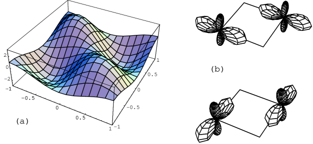
Figure 7: Orbital superexchange $J_{\tau}$ for a single pair along $XY$ (see figure 1): (a) bond energy as a function of the orbital angles $\theta_{1}$ and $\theta_{2}$ (energy in units of $\frac{1}{4}J_{\tau}$, angles in units of $\pi$); (b) the two favoured pairs of occupied $e_{g}$ orbitals.

Frustration prevents this optimum orbital arrangement to be realized on all bonds simultaneously, as already pointed out by MK. As will be seen in the next section, on the full triangular lattice the orbital interaction favours phases in which a pair has either a ferro orbital (FO) arrangement at a general angle $\theta\equiv\theta_{i}=\theta_{j}$ or similarly a canted orbital (CO) arrangement with $\theta\equiv\theta_{i}=-\theta_{j}$. It is therefore of interest to consider the effective spin-spin interactions realized under those conditions.

Quite generally, once the orbitals of the pair are fixed, supposedly determined by the pure orbital interaction, the resulting effective spin SE interaction can be written as a Heisenberg Hamiltonian,

$${\mathcal{H}}_{\rm spin}^{\rm eff}(\theta_{i},\theta_{j})=\sum_{\langle ij\rangle}J_{ij}^{\rm eff}(\theta_{i},\theta_{j})\>{\bi S}_{i}\cdot{\bi S}_{j},$$ (53)

with the effective spin SE coupling $J_{ij}^{\rm eff}$ given by

$$J_{ij}^{\rm eff}(\theta_{i},\theta_{j})=-{\textstyle\frac{1}{4}}\Big{[}4J_{\sigma}-J_{\mu}\Big{(}1+2\cos^{2}\theta_{-}-4\cos^{2}(\theta_{+}+\chi_{\gamma})\Big{)}-4J_{\nu}\cos(\theta_{+}+\chi_{\gamma})\cos\theta_{-}\Big{]},$$ (54)

where $\theta_{\pm}=(\theta_{i}\pm\theta_{j})/2$, as obtained by inserting equations (14) and (15) into (50). For the two relevant cases of orbital order one thus finds, by adopting the appropriate values for the angles $\theta_{i}$ and $\theta_{j}$,

$$J_{\rm FO}(\theta)\equiv J_{ij}^{\rm eff}(\theta,\theta)=-{\textstyle\frac{1}{4}}\Big{[}4J_{\sigma}-3J_{\mu}+4J_{\mu}\cos^{2}(\theta+\chi_{\gamma})-4J_{\nu}\cos(\theta+\chi_{\gamma})\Big{]},$$ (55)

$$J_{\rm CO}(\theta)\equiv J_{ij}^{\rm eff}(\theta,-\theta)=-{\textstyle\frac{1}{4}}\Big{[}4J_{\sigma}-(1-4\cos^{2}\chi_{\gamma})J_{\mu}-2J_{\mu}\cos^{2}\theta-4\cos\chi_{\gamma}J_{\nu}\cos\theta\Big{]}.$$ (56)

The dependence on $\theta$ is shown in figure 8 for the values of $J_{\sigma}$, $J_{\mu}$ and $J_{\nu}$ obtained with our standard parameter set. Figure 8(a) shows that in the FO case the spin SE constant is mostly FM (negative), as expected from the Goodenough-Kanamori-Anderson rules, but that AF values, though smaller, are indeed possible, notably for orbitals with $\theta\simeq\pm\pi/3$. Note that the coupling constant is that for a bond along $XY$; equation (55) shows that the curve should be shifted by $\pm 2\pi/3$ for bonds along $YZ$ or $ZX$. The CO case is shown in figure 8(b), for a bond in the $YZ$ or $ZX$ direction while the angle is still given with respect to the basis {$|iz\rangle$, $|i\bar{z}\rangle$} as in equations (1) and (2). Note that the coupling can again be AF as well, precisely for those angles ($\theta\simeq\pm\pi$) where the FO arrangement gives the largest FM coupling in the $XY$ direction.

Figure 8: Effective spin-spin superexchange constant (in units of $J$) versus angle $\theta$ (in units of $\pi$; see equation (2)): (a) For a single pair along $XY$ for ferro orbitals ($\theta=\theta_{i}=\theta_{j}$); (b) For a single pair along $YZ$ or $ZX$ for canted orbitals ($\theta=\theta_{j}=-\theta_{j}$).

6 Possible ground states

We have already noticed that the orbital SE is strongly frustrated — since the specific orbitals minimizing the pair energy are different for each bond direction, the interactions between neighboring Ni ions cannot be satisfied in all three bond directions simultaneously. The fact that frustration occurs although the interaction is of ferro type is somewhat unusual and is generic for orbital physics as compared to spin physics. The underlying reason is that the orbital interaction Hamiltonian (49) does not have global continuous rotational $U(1)$ symmetry with regard to the orbital angles $\theta_{i}$, but is only invariant under rotation by an angle $\pm 2\pi/3$, corresponding to a cyclic permutation of the bond directions $XY$, $YZ$ and $ZX$. This characteristic feature and the ensuing frustration are not captured by $SU(4)$ symmetric models [32, 33].

Next we consider what states with long-range order (LRO) are possible. As pointed out by MK, the simplest such state, viz. with uniform ferro orbital order, is actually a minimum energy state in MF theory. Its energy is independent of $\theta$ and equal to $-{\textstyle\frac{3}{4}}J_{\tau}$ per site, while moreover this FO phase may be interrupted without energy cost by lines in which all orbitals have the opposite angle $-\theta$, i.e. by canting of all orbitals along a line in the triangular lattice. In order to see how this comes about, one may write down the energy for a set of FO lines (for definiteness along the $XY$ direction) with orbitals in line $n$ given by $\theta_{n}$. From (49) and (15) one obtains

$$E_{\rm FO-l}=E_{\rm intraline}+E_{\rm interline}$$

$$\hbox to0.0pt{\hss${}={}$}{\textstyle\frac{1}{4}}J_{\tau}\sum_{n}[2\cos 2\theta_{n}-1]$$

$$+{\textstyle\frac{1}{2}}J_{\tau}\sum_{n}\Big{[}\cos\,(\theta_{n}+\theta_{n+1}-{\textstyle\frac{2\pi}{3}})+\cos\,(\theta_{n}+\theta_{n+1}+{\textstyle\frac{2\pi}{3}})-\cos\,(\theta_{n}-\theta_{n+1})\Big{]}$$

$$\hbox to0.0pt{\hss${}={}$}{\textstyle\frac{1}{4}}J_{\tau}\sum_{n}[4\cos^{2}\theta_{n}-3]-J_{\tau}\sum_{n}\cos\theta_{n}\;\cos\theta_{n+1}$$ (57a)

$$\hbox to0.0pt{\hss${}={}$}{\textstyle\frac{1}{4}}J_{\tau}\sum_{n}\Big{[}2(\cos\theta_{n}-\cos\theta_{n+1})^{2}-3\Big{]}.$$ (57b)

Equation (57a) shows that upon variation of the angles $\theta_{n}$ the gain in intraline line energy is compensated by a loss in interline energy, leading on balance to $E_{\rm FO-l}$ being not dependent on the value of $\theta$ in the ordered phase, while equation (57b) shows that for any two neighbouring lines the same energy is obtained for $\theta_{n}=+\theta_{n+1}$ and $\theta_{n}=-\theta_{n+1}$. So in addition to the degeneracy with respect to $\theta$ generated by the frustration, the model also gives rise to randomness due to uncorrelated switches from $+\theta$ to $-\theta$ between successive lines. Such a random CO phase is probably best interpreted as the occurrence of twin boundaries or antiphase boundaries between equivalent FO domains. Because of the zero energy cost for formation of a boundary there is actually no preference for the formation of large domains.

It was argued by MK that the degeneracy in $\theta$ is an artefact of MF theory, and that this $U(1)$ symmetry of the FO state, not present in the original Hamiltonian (49), would be lifted in the FO domains by the ‘order-out-of-disorder’ mechanism [34], and that in this way the threefold symmetry associated with the triangular lattice would be restored. However, as the energies involved in the restoring quantum fluctuations are generally small, only a fraction of the orbital coupling constant $J_{\tau}$, one should at this stage reconsider the orbital-spin coupling. Even though the relevant coupling constants $J_{\sigma}$, $J_{\mu}$ and $J_{\nu}$ are much smaller than $J_{\tau}$, the spin-and-orbital dependent SE energy might still be more significant than the fluctuation energies in lifting the $\theta$ degeneracy. Figure 8 suggests that it could do so already at the MF level and so determine the ground state before fluctuations need to be considered.

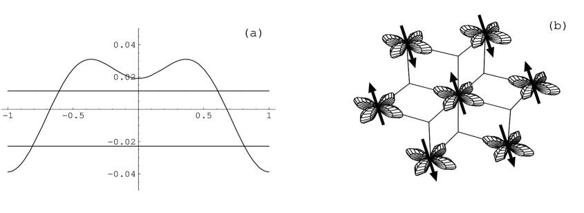
Figure 9: Spin-and-orbital order: (a) MF energy per site (in units of $J=t^{4}/\Delta^{3}$) for various ordered phases as function of the orbital angle $\theta$: (upper horizontal line:) ferro-orbital / 120^∘ spin order ; (lower horizontal line:) ferro-orbital / ferromagnetic order, degenerate with orbital-line / ferromagnetic order; (curve:) ferro-orbital/ spin-line order, degenerate with orbital-line / spin-line order; (b) Ground state in mean field: ferro-orbital order of $d_{x^{2}-y^{2}}$ orbitals with spin-line order (along the $XY$ direction).

We therefore consider the following LRO spin patterns in conjunction with orbital order: (i) FM order; (ii) the 120^∘ three-sublattice order which is the ground state of the classical TALAF; (iii) AF line order similar to that of the orbitals, i.e. lines of parallel spins along the same direction as the orbital lines, and the spins alternating between up and down on successive lines. The result for the MF energy is shown in figure 9(a). It turns out that indeed the $\theta$ degeneracy is lifted, and the lowest MF energy is seen to be obtained for FO order with orbital angle $\theta=+\pi$ (or $\theta=-\pi$), corresponding to a $d_{x^{2}-y^{2}}$ orbital at every site, in combination with spin AF line order, illustrated in figure 9(b). This shows that even though the spin-orbital interaction is considerably weaker than the pure orbital interaction, it can still have a qualitative effect on the nature of the ground state by breaking the $U(1)$ symmetry generated by the orbital interactions alone and restoring threefold symmetry. Therefore the large difference in coupling strength does not necessarily lead to a decoupling of the spin and orbital degrees of freedom.

Remarkably, the $+\theta$/$-\theta$ twin-boundary degeneracy persists, not only at the optimum angle $\pm\pi$, where it is immaterial since it corresponds only to a sign change of the orbital wavefunctions, but also at arbitrary $\theta$. This could in fact have been recognized from the $\theta$ dependence of the effective spin exchange constants: the spin exchange in the transverse direction (on the bonds along $YZ$ and $ZX$) as given for the FO case by shifts over $\pm{\textstyle\frac{2\pi}{3}}$ in figure 8(a) is the same as that given for the CO case in figure 8(b).

Most significantly, we note that both for the ordered FO phase and for the disordered CO phase the effective spin-spin exchange is antiferromagnetic in the transverse direction, also for orbital angles deviating somewhat from the optimum value $\pm\pi$. However, for a disordered phase with truly random orbital angles, either a paraorbital state at high temperature or an orbital glass, the situation would be very different. Figure 8 indicates that orbital randomness would produce a wide distribution of mostly FM exchange constants, although small AF values would still occur but not in a regular pattern as in the FO and CO phases. Obviously a phase transition to an orbital ordered phase would manifest itself also in the magnetic properties, e.g. in the dispersion of spin waves.

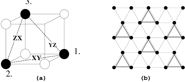
Figure 10: Geometry relevant for the orbital valence bond (OVB) state: (a) Triangular three-site plaquette in a Ni plane for determination of the exact eigenstates of the orbital interaction; (b) Lattice covering with three-site plaquettes in the OVB state.

Whereas the above analysis shows that the spin-orbital interaction could support orbital LRO, the degeneracy in the orbital sector and the small MF energy of only $-{\textstyle\frac{1}{4}}J_{\tau}$ per bond, both for the FO and for the CO phase, raise the question whether orbital LRO by itself is stable against formation of a disorded state of valence bond (VB) type. We therefore studied orbital valence bond (OVB) states [15, 32] in the following way. First we solved the eigenvalue problem of the orbital SE Hamiltonian ${\mathcal{H}}_{\rm eff,o}$ exactly on the three-site triangular plaquette shown in figure 10(a). The eigenstates are four doublets, with ground state energy $E_{0}^{\rm plaq}=-{\textstyle\frac{3}{2}}J_{\tau}$ and excited states at $-J_{\tau}$, $+{\textstyle\frac{1}{2}}J_{\tau}$ and $+2J_{\tau}$, the ground state doublet being

$$|e_{1}\rangle=\sqrt{{\textstyle\frac{4}{7}}}(|x\rangle_{1}|z\rangle_{2}|y\rangle_{3}+|z\rangle_{1}|y\rangle_{2}|x\rangle_{3}),$$

$$|e_{2}\rangle=\sqrt{{\textstyle\frac{4}{7}}}(|\bar{x}\rangle_{1}|\bar{z}\rangle_{2}|\bar{y}\rangle_{3}+|\bar{z}\rangle_{1}|\bar{y}\rangle_{2}|\bar{x}\rangle_{3}).$$ (57bf)

Note that particular combinations of orbitals are favoured, similar to the orbital order for the V triangle in LiVO₂ [35]. It is remarkable that on a triangular lattice such triangular VB correlations in orbital space are favoured, in contrast to dimer singlet correlations in spin systems [36].

We then constructed an OVB solid by covering the triangular lattice with three-site plaquettes, as in figure 10(b), and assigning to each triangular plaquette $l$ an orbital wavefunction built from the groundstate components (57bf),

$$|\Delta_{l}\rangle=\cos\theta_{l}\,|e_{1}\rangle_{l}+\sin\theta_{l}\,|e_{2}\rangle_{l},$$ (57bg)

with $\theta_{l}$ still to be determined. This amounts to assigning a fictitious spin to each plaquette and solving a frustrated spin problem on the triangular lattice. In MF theory the total energy is now given by addition of the groundstate energies from all plaquettes and the interplaquette energies coming from the two bonds between nearest neighbour plaquettes,

$$E_{\rm OVB}=\sum_{l}E_{\Delta_{l}}+\sum_{l,m}\langle\Delta_{l},\Delta_{m}|{\mathcal{H}}_{\rm eff,o}|\Delta_{l},\Delta_{m}\rangle=\sum_{l}E_{0}^{\rm plaq}+\sum_{l,m}E_{\rm VB}^{\rm p-p}(\theta_{l},\theta_{m}).$$ (57bh)

For a uniform solution the energy per bond is given by

$$\bar{E}_{\rm OVB}={\textstyle\frac{1}{6}}\Big{(}2\times{\textstyle\frac{1}{3}}\times E_{0}^{\rm plaq}+4\times{\textstyle\frac{1}{2}}\times E_{\rm VB}^{\rm p-p}\Big{)},$$ (57bi)

by counting the number of intraplaquette and interplaquette bonds. Although the plaquette eigenenergy amounts to ${\textstyle\frac{1}{3}}E_{0}^{\rm plaq}=-{\textstyle\frac{1}{2}}J_{\tau}$ per bond of the plaquette, which for this exact solution is of course lower than the energy per bond for the FO and CO phases, the plaquettes cover only one third of the bonds of the lattice, and so the contribution from the interplaquette energy $E_{\rm VB}^{\rm p-p}$ is decisive.

The optimum values of the plaquette angles are found to be $\theta_{l}=+{\textstyle\frac{\pi}{4}}$, $\theta_{m}=-{\textstyle\frac{\pi}{4}}$, for which $E_{\rm VB}^{\rm p-p}=-{\textstyle\frac{27}{49}}J_{\tau}$, and if this value could be attained between any pair of plaquettes one would have $\bar{E}_{\rm OVB}=-({\textstyle\frac{1}{6}}+{\textstyle\frac{9}{49}})J_{\tau}\simeq-0.3503J_{\tau}$, lower than $\bar{E}_{\rm FO}=\bar{E}_{\rm CO}=-0.25J_{\tau}$. However, this would requiring alternating angles $\pm{\textstyle\frac{\pi}{4}}$, which is impossible because of frustration on the triangular lattice. The optimum value that can be obtained is $\bar{E}_{\rm OVB}\simeq-0.228J_{\tau}$, realized for instance by line order of $\pm{\textstyle\frac{\pi}{4}}$. This is remarkably close to the energy per bond of the site-ordered states, and just confirms that the orbital sector is strongly frustrated. It is therefore likely that some quenched disorder would suffice to turn the system into an orbital glass below a freezing temperature $T_{\rm of}$ determined by $J_{\tau}$, as proposed to explain the behaviour of the orbitals observed in LiNiO₂ [10].

7 Origin of the difference between LiNiO₂ and NaNiO₂

In view of the above results the properties of LiNiO₂ are puzzling [9, 10], as neither orbital nor spin order sets in down to the lowest temperatures. Thus the high degeneracy of the ground state manifold apparently persists, with Ni³⁺ ions being in the low-spin ($t_{2g}^{6}e_{g}^{1}$) state, with twofold orbital and twofold spin degeneracy. The standard scenario for such ions would be a cooperative Jahn-Teller effect lifting the orbital degeneracy below a structural transition at $T_{s}$, followed by a magnetic transition at $T_{N}$, lifting also the degeneracy in spin space. Both transitions could be induced already by the electronic mechanism involved in the SE, but the interactions with the lattice are expected to play a significant role in the structural transition, enhancing the value of $T_{s}$, as found in the manganites [37]. In spite of the strong orbital interactions reported above, and although the $S=1/2$ spins interact by the predominantly FM SE described in the previous sections, and the magnetic susceptibility follows the Curie-Weiss behaviour, $\chi\propto(T-\theta_{\rm CW})^{-1}$ with $\theta_{\rm CW}\sim 35$ K down to about 80 K [4, 5, 6], long-range order in either orbital or spin space is absent [7, 9]. This would suggest that the $e_{g}$ orbital degree of freedom plays an important role, possibly stabilizing strong singlet orbital correlations on individual bonds, and supporting a spin liquid state [15].

Before addressing the central question of the origin of the spin liquid state in LiNiO₂, let us summarize shortly the structural and magnetic properties of the similar NaNiO₂ compound, which crystallizes in the same structure as LiNiO₂ (see figure 1). The standard scenario with two subsequent transitions described above is indeed realized in NaNiO₂. The latter compound undergoes a first-order cooperative Jahn-Teller transition lowering the local symmetry from trigonal to monoclinic at $T_{s}=480$ K [38], and the Ni-O distances change from $d=1.98$ Å to two long bonds with $d=2.14$ Å and four short bonds with $d=1.91$ Å at $T<T_{s}$. In the low-temperature phase a magnetic transition at $T_{N}=20$ K to an $A$-type AF insulator follows — it was first derived from magnetization measurements on a single crystal by Bongers and Enz already in 1966 [39]. This magnetic phase has also been confirmed by a complete static and dynamic magnetic study at low temperatures, where strong anisotropy between the effective magnetic interactions was established [38]. An FM intralayer coupling of $J_{\rm FM}=-26$ K and a weak AF interlayer coupling of $J_{\rm AF}=2$ K were found, values consistent with the observed Curie-Weiss temperature $\Theta=35$ K and Néel temperature $T_{N}=20$ K. Similar values of the exchange constants ($J_{\rm FM}\simeq-29$ K and $J_{\rm AF}\simeq 1.9$ K) were also deduced recently by analyzing the dispersion of spin waves found in neutron scattering experiments [40]. We remark that the parameters which fit the Curie-Weiss law change around the structural transition at $T_{s}$ [38], which indicates that the magnetic couplings depend on the actual orbital state, in agreement with the model presented here.

In contrast, in LiNiO₂ the structural transition is absent, but EXAFS experiments indicate the presence of local Jahn-Teller distortions below an orbital freezing temperature $T_{\rm of}\sim 400$ K, with two different Ni-O distances again favouring occupied directional $d_{3z^{2}-r^{2}}$-type orbitals [41]: two long bonds with $d=2.09$ Å and four short bonds with $d=1.91$ Å. While these local distortions are similar to those observed in NaNiO₂, the absence of a macroscopic distortion in LiNiO₂ has been a mystery since its synthesis [1]. However, very recent evidence from neutron diffraction indicates that below $T_{\rm of}$ the orbitals actually develop short-to-medium-range order in a trimerized state, although the associated strain field prevents the ordering from becoming long-range, and instead nanoscale domains of local orbital trimer order are formed [42]. Nevertheless, even local distortions favouring occupied $d_{3z^{2}-r^{2}}$ orbitals are intriguing, as we have seen above that the SE favours instead alternating symmetric and antisymmetric combinations of the basis orbitals, $d_{3z^{2}-r^{2}}\pm d_{x^{2}-y^{2}}$, for individual Ni³⁺-Ni³⁺ pairs (so e.g. in a disordered state), and FO order of $d_{x^{2}-y^{2}}$ orbitals, as obtained in the MF approximation. Actually, such an ordered phase with occupied $d_{x^{2}-y^{2}}$ orbitals has been observed in large magnetic field [8], which demonstrates that the state predicted by the SE model is energetically close to the actual ground state, and a quantum phase transition between different orbital states can be triggered by an applied magnetic field. The very fact that instead, in the absence of a magnetic field, local distortions of NiO₆ octahedra associated with occupied $d_{x^{2}-y^{2}}$-type orbitals dominate at low temperature, we interpret as a strong indication that the orbital physics is in the end determined by the Jahn-Teller coupling to the lattice and not by the orbital SE.

The ground state of LiNiO₂ remains the subject of intense debate. Several mechanisms for the spin liquid phase have been proposed so far: ($i$) quantum fluctuations on AF bonds [15], ($ii$) geometrical frustration of AF interactions in the $SU(4)$ spin-orbital model on the triangular lattice [32, 33], ($iii$) decoupling of spin and orbital degrees of freedom because of the large difference, confirmed above, between orbital and spin-orbital SE coupling constants [2], ($iv$) disorder due to Ni²⁺ ions in the Li planes [8, 9]. Interestingly, also in the $SU(4)$ model both AF and FM interactions are allowed [32, 33], so at first sight the mechanism ($ii$) might appear similar to the present model of section 4. However, the $e_{g}$ orbital operators do not respect $SU(2)$ symmetry, and thus the actual magnetic interactions which follow from the $SU(4)$ model are quite different. For instance, in the $SU(4)$ model one may assume perfect FO order, with $\langle{\bi T}_{i}\cdot{\bi T}_{j}\rangle=\frac{1}{4}$ for the orbital operators on each bond $\langle ij\rangle$, which would give AF spin interactions on all the bonds, while such a situation cannot be realized for $e_{g}$ orbitals. Also a state with the orbitals staggered for all bonds is not allowed on a triangular lattice. Therefore, we suggest that the role of geometrical frustration of magnetic interactions is overestimated in the $SU(4)$ model and cannot explain the properties of the triangular Ni planes by itself. In contrast, all other mechanisms could contribute and stabilize the spin liquid state in a 3D lattice of LiNiO₂. We propose a new scenario below in which the above aspects (iii) and (iv) are supplemented by two important features of the orbital glass [10] or trimer nanodomain state [42] below the transition at $T_{\rm of}\simeq 400$ K: ($v$) the weakness of the (effective) SE interactions between Ni³⁺ ions in adjacent Ni planes, and ($vi$) the Jahn-Teller coupling to the lattice, which induces local distortions favouring directional $d_{3z^{2}-r^{2}}$-like orbitals.

We emphasize that the experimental studies on NaNiO₂ and LiNiO₂ have identified two competing effects which operate in triangular 2D Ni planes: on the one hand local Jahn-Teller distortions favouring occupied $d_{3z^{2}-r^{2}}$ orbitals, produced by the on-site Jahn-Teller coupling, and on the other hand the SE, which would instead stabilize orbital order with occupied $d_{x^{2}-y^{2}}$ orbitals, coexisting with FM interactions within the planes. Although Ni-Ni distances and Ni-O-Ni bond angles in the O–Ni–O trilayers of the two compounds are similar, it may well be that the in-plane elastic couplings and orbital SE differ just sufficiently that the 2D orbital susceptibilities are qualitatively different. In particular, the competition between Jahn-Teller effect and SE may favour orbital disorder or complex multiple-sublattice orbital order when one interaction is only marginally stronger than the other one. This is in fact suggested by the behaviour of LiNiO₂ in magnetic field, mentioned above, and by the properties of the mixed compound Li_0.3Na_0.7NiO₂ [43], discussed below. Whether orbital and magnetic order stabilize in a 3D system, however, depends also crucially on the interplane interactions. Without any coupling between the planes, no long-range order could occur in the 2D planes anyway, in accordance with the Mermin-Wagner theorem.

One thus expects that 3D orbital order can be induced only by a sufficiently strong effective interplane coupling, as apparently encountered in NaNiO₂, while the absence of orbital order observed in Li_1-xNi_1+xO₂ may be explained by a weaker effective interplane coupling in combination with an already weaker in-plane ordering tendency. Even without an explicit extension of the present microscopic spin-orbital model we can already suggest two mechanisms responsible for this weak interlayer coupling. First of all, the interplane SE is intrinsically weaker in LiNiO₂ than in NaNiO₂ because of the different covalency of the Ni–O–Li–O–Ni bonds as compared to the Ni–O–Na–O–Ni bonds, owing to the weaker hybridization between the oxygen $2p$ orbitals and the spatially less extended Li $2s$ orbitals than between the oxygen $2p$ orbitals and the bigger Na $3s$ orbitals. Although this difference is quantitative, it may lead to a qualitatively different behaviour. A further point is then how the individual Ni³⁺-Ni³⁺ orbital interactions between two neighbouring planes add up. For two orbital ordered planes, as in NaNiO₂, the interactions add up coherently, but if the orbitals preferentially avoid ordering in each Ni plane, e.g. because of a tendency towards domain formation, then in spite of the intrinsically identical spin-orbital interaction between Ni³⁺ ions in adjacent Ni planes, orbital (and magnetic) couplings add up incoherently. Second, it is well known that in the case of NaNiO₂ an almost ideal structure is obtained, while Li_1-xNi_1+xO₂ is never stoichiometric and extra Ni ions occur in Li planes [9]. This creates frustration due to extrinsic randomness in the individual interplane interactions, and thus further weakens the effective interplane coupling.

Finally, the absence of 3D magnetic order in LiNiO₂ is apparently similarly due to the weakness of the magnetic effective interplane coupling. While it is tempting to ascribe it instead to the presence of both AF and FM SE interactions in the triangular Ni planes, demonstrated above in the spin-orbital model, this is unlikely to be the leading effect stabilizing the spin liquid. In particular, in the orbital glass state the SE would be FM on by far the majority of the bonds in the Ni planes, as follows from equation (54) [compare also figure 8], with the precise fraction depending on the degree of disorder, while moreover the few AF interactions would be much weaker than the FM interactions. That the effective interplane magnetic coupling in LiNiO₂ is weak, is not only due to the interplane SE being intrinsically weak owing to the small covalency. In addition, in spite of the identical spin-orbital interaction between Ni³⁺ ions in adjacent Ni planes, the absence of orbital long-range order in the Ni planes will make individual Ni³⁺-Ni³⁺ spin-spin SE interactions add up incoherently.

An additional extrinsic mechanism opposing magnetic order is provided by magnetic interactions due to the Ni²⁺ defects in the Li planes, which by themselves frustrate weak AF SE interactions by stronger FM interactions along Ni³⁺-Ni²⁺-Ni³⁺ units [9, 11], additionally enhanced due to the $S=1$ spin states involved. As long as such defects do not occur, coherence in the magnetic interplane coupling is easier to obtain. Our scenario is not inconsistent with the recent observation of the decoupling of orbital and spin degrees of freedom in the mixed compound Li_0.3Na_0.7NiO₂ which has a very different orbital state and yet a similar magnetic ground state as NaNiO₂ [44], with similar exchange constants [43].

8 Discussion and summary

The above analysis demonstrates that the qualitative properties which follow from orbital and spin correlations within triangular Ni planes with 90^∘ Ni–O–Ni bonds can be understood within a realistic spin-orbital SE model. This model demonstrates, in agreement with the SE model of Mostovoy and Khomskii [2] and with experiment [10], that the orbital SE $J_{\tau}$ is stronger by one order of magnitude than any other (pure spin or spin-orbital) interaction, because all magnetic dependence for the SE along Ni–O–Ni bonds originates from the singlet-triplet splitting of the oxygen $2p^{4}$ configuration, and is therefore smaller by at least a factor $J_{p}/U_{p}\sim 0.1$, where $U_{p}$ ($J_{p}$) is the interorbital Coulomb (Hund’s exchange) interaction on oxygen. These parameters, as well as the effective hopping $t$ and the charge transfer energy $\Delta$, are of importance to establish quantitative consequences of the SE model, in particular on such magnetic properties as the effective exchange constants and the magnetic susceptibility.

The orbital SE has interesting consequences for the orbital state and also for the magnetic interactions within the triangular Ni planes. First of all, for an individual (NiO)₂ plaquette (figure 7), a pair of identical orbitals, either both $d_{3z^{2}-r^{2}}+d_{x^{2}-y^{2}}$ or both $d_{3z^{2}-r^{2}}-d_{x^{2}-y^{2}}$, is favoured. Therefore, in MF approximation a symmetry broken state arises in the Ni planes, with FO order characterized by a single orbital angle $\theta$ [as defined in equation (2)] along a particular direction. This is in contrast with the behaviour obtained for the cuprates [19] or the manganites [37], where orbitals with angles $\theta$ and $-\theta$ alternate on interlacing sublattices. As a result, one expects domains with either $|\theta\rangle$ or $|-\theta\rangle$ orbitals, separated by twin-boundaries. Even though much weaker than the orbital SE, the spin-orbital SE plays a crucial role in the selection of the ground state. It breaks the $U(1)$ symmetry generated in MF theory by the orbital SE and restores the original threefold symmetry with respect to the orbital angle $\theta$. By this mechanism FO order with planar $d_{x^{2}-y^{2}}$ orbitals in the triangular Ni planes is stabilized in MF theory. A characteristic feature of this state is the presence of both FM and AF spin interactions.

After having a closer look at the magnetic properties of LiNiO₂, we suggest that this compound represents an interesting case of competition between the type of orbitals favoured locally by the Jahn-Teller effect and those favoured by the SE in an $e_{g}$ system with 90^∘ Ni-O-Ni bonds, and that this is likely to induce orbital disorder. Remarkably, this case is reminiscent of the situation encountered in the $t_{2g}$ orbital model [20, 45], and contradicts the experience and common knowledge from the $e_{g}$ models in perovskites, where the SE along 180^∘ bonds favours alternating orbitals and both mechanisms support each other [37, 46]. Whether this competition might lead to dynamical disorder certainly depends on the phonons, and we conclude that further study of elastic coupling and phonons is urgently needed.

Summarizing, we presented and discussed the consequences of the 2D frustrated quantum spin-orbital model derived for the triangular Ni planes of two compounds with a very different behaviour: LiNiO₂ and NaNiO₂. This model emphasizes the importance of charge transfer (Goodenough) processes and presents a complete description of the superexchange interactions on the 90^∘ Ni-O-Ni bonds in triangular Ni planes, so we are confident that it provides a solid starting point for future progress in the theory. The frustration in the orbital sector is not of Ising type, as suggested before [10], but due to different orbitals being favoured for different bond directions. Providing a final answer concerning the origin of the different magnetic properties of LiNiO₂ and NaNiO₂ requires an extension of the present microscopic model by a microscopic description of both the interlayer coupling and of the coupling between orbitals and the lattice. We identified two possible reasons why the interlayer (spin and orbital) coupling is so weak: ($i$) an intrinsic effect due to the small covalency of interplane Ni–O–Li–O–Ni bonds, and ($ii$) an extrinsic effect due to Ni disorder in Li_1-xNi_1+xO₂ — both these effects are expected to play an important role and to be responsible for the absence of $A$-type antiferromagnetic order in LiNiO₂.

Appendix A Derivation of the spin-orbital Hamiltonian

Figure 11: Example of superexchange processes (arrows in clockwise direction) of $M$-type along the $XY$ direction. — After the first transition (top) either the triplet $T$ or the orbital doublet $D$ is reached at what is now a Ni²⁺ ion, while the second transition (bottom right) gives either the orbital doublet $D$ or the singlet $S$ at the other Ni²⁺ ion. The corresponding double excitation into the $2p^{4}$ configuration at oxygen is either to the triplet $t$ or the singlet $s$. — Deexcitation occurs by the reverse transitions, either in the same or in reversed order (shown in the diagram).

Here we give further details on the derivation of the spin-orbital Hamiltonian ${\mathcal{H}}_{\rm eff}$, in particular regarding the case where $J_{\rm H}$ is finite. First we take a closer look at the four-step charge transfer sequences. As an example, let us consider (see figure 11) a Ni–Ni pair in the $XY$ direction in an M-type initial configuration with the electron on Ni-site $i$ ($j$) in the non-hopping $d_{z^{2}-x^{2}}$ orbital $|\bar{y}\rangle_{i}$ (hopping $d_{3x^{2}-r^{2}}$ orbital $|x\rangle_{j}$) having spin up (down), i.e. an initial state $|{\rm M},\uparrow\downarrow\rangle$, and the electrons being transferred from the oxygen having opposite spin. In an obvious notation the corresponding contribution to ${\mathcal{H}}_{\rm eff}$ is $\lshad{\rm M},\uparrow\downarrow;\downarrow\uparrow\rshad\;{\mathcal{P}}_{i}^{\bar{y}}\,{\mathcal{P}}_{j}^{x}\>{\bi Q}_{ij}^{\uparrow\downarrow}$. In the middle intermediate state the ion states $T$ and $D$, $t$ and $s$, and $D$ and $S$ occur with equal amplitude at the Ni²⁺, O⁰ and Ni²⁺ ions, respectively. Denoting the contribution from a doubly excited state by $[XvY]$, with $X,Y\in\{T,D,S\}$ and $v\in\{t,s\}$, the contribution corresponding to figure 11 is thus given by

$$\lshad{\rm M},\uparrow\downarrow;\downarrow\uparrow\rshad={\textstyle\frac{1}{2}}\Big{(}[TtD]+[TtS]+[DtD]+[DtS]+[TsD]+[TsS]+[DsD]+[DsS]\Big{)},$$

where again a factor 4 has already been included. However, the four sequences that lead to a particular middle state upon inverting the order of the exciting and/or deexciting charge transfers, are now in general inequivalent, as illustrated by the tree diagram of figure 12, because the energies of the first and third intermediate state may depend upon the sequence. The contributions $[XvY]$ therefore need to be expanded as

$$\hskip 28.45274pt[XvY]={\textstyle\frac{1}{4}}\Big{[}(X|XvY|X)+(X|XvY|Y)+(Y|XvY|X)+(Y|XvY|Y)\Big{]},$$ (57bj)

where we denote in $(Z_{1}|XvY|Z_{3})$ by $Z_{1}$ ($Z_{3}$) the state reached after the first (third) charge transfer step.

Figure 12: Diagrammatic representation of the superexchange processes shown in figure 11, including inverted order of excitation and deexcitation processes.

The explicit expression for this quantity is [compare equation (30)]

$$(Z_{1}|XvY|Z_{3})=-\frac{t^{4}}{\Delta_{Z_{1}}\Delta_{Z_{3}}(\Delta_{X}+\Delta_{Y}+U_{v})}+\frac{t^{4}}{\Delta_{Z_{1}}\Delta_{Z_{3}}(\Delta_{X}+\Delta_{Y})}$$

$$=\frac{t^{4}\>U_{v}}{\Delta_{Z_{1}}\Delta_{Z_{3}}(\Delta_{X}+\Delta_{Y})(\Delta_{X}+\Delta_{Y}+U_{v})},$$ (57bk)

where the second term in the first line is the renormalization correction discussed in section 3. Inserting (57bk) into equation (57bj) one now obtains

$$[XvY]=\frac{t^{4}}{4}\;\frac{\Delta_{X}+\Delta_{Y}}{\Delta_{X}^{2}\>\Delta_{Y}^{2}}\;\frac{U_{v}}{\Delta_{X}+\Delta_{Y}+U_{v}},$$ (57bl)

so that for example

$$[TsS]=\frac{t^{4}\>\Delta}{2(\Delta^{2}-4J_{\rm H}^{2})^{2}}\;\frac{U_{p}+J_{p}}{2\Delta+U_{p}+J_{p}},$$ (57bm)

$$[DtD]=\frac{t^{4}}{2\Delta^{3}}\;\frac{U_{p}-J_{p}}{2\Delta+U_{p}-J_{p}}.$$ (57bn)

The next step consists in listing all possible initial configurations and for each one the allowed spin arrangements of the two hopping electrons, and then working out, as above for $\lshad{\rm M},\uparrow\downarrow;\downarrow\uparrow\rshad$, with the help of diagrams like those shown in figure 11, which middle intermediate states contribute. The result is shown in table 1, which gives the coefficients $C(..|..)$ in

$$\lshad{\rm L},\sigma\sigma^{\prime};\bar{\sigma}\bar{\sigma}^{\prime}\rshad=\sum_{X,Y,v}C({\rm L},\sigma\sigma^{\prime};\bar{\sigma}\bar{\sigma}^{\prime}|XvY)\,[XvY].$$ (57bo)

The SE coupling constants $\{K_{\rm L}^{\rm T,S}\}$ for spin triplet and spin singlet, appearing in equation (33), are now obtained as follows. In each case (L = O, M or N) consider first the $m=1$ component of the triplet, i.e. the row(s) in table 1 in which there is an up-spin on both Ni³⁺ ions. Adding them gives the triplet contribution $K_{\rm L}^{\rm T}$, while similarly adding the row(s) for which the two Ni³⁺ spins are in up-down configuration gives $K_{\rm L}^{\uparrow\downarrow}$,

$$K_{\rm L}^{\rm T}=\sum_{\bar{\sigma},\bar{\sigma}^{\prime}}\lshad{\rm L},\uparrow\uparrow;\bar{\sigma}\bar{\sigma}^{\prime}\rshad=\sum_{\bar{\sigma},\bar{\sigma}^{\prime}}\;\sum_{X,Y,v}C({\rm L},\uparrow\uparrow;\bar{\sigma}\bar{\sigma}^{\prime}|XvY)\,[XvY],$$ (57bp)

$$K_{\rm L}^{\uparrow\downarrow}=\sum_{\bar{\sigma},\bar{\sigma}^{\prime}}\lshad{\rm L},\uparrow\downarrow;\bar{\sigma}\bar{\sigma}^{\prime}\rshad=\sum_{\bar{\sigma},\bar{\sigma}^{\prime}}\;\sum_{X,Y,v}C({\rm L},\uparrow\downarrow;\bar{\sigma}\bar{\sigma}^{\prime}|XvY)\,[XvY].$$ (57bq)

As $K_{\rm L}^{\uparrow\downarrow}$ corresponds to the $m=0$ components and so is shared between singlet and triplet, one now obtains the singlet contribution from $K_{\rm L}^{\rm S}=2K_{\rm L}^{\uparrow\downarrow}-K_{\rm L}^{\rm T}$.

Table 1: Coefficients $C({\rm L},\sigma\sigma^{\prime};\bar{\sigma}\bar{\sigma}^{\prime}|XvY)$ specifying the contributions to the superexchange Hamiltonian according to equation (57bo). Here ${\rm L},\sigma\sigma^{\prime}$ denotes the initial configuration and $\bar{\sigma}\bar{\sigma}^{\prime}$ the spins of the transferred electrons, with ${\rm L}\in\{{\rm O},{\rm M},{\rm N}\}$ and $\sigma,\sigma^{\prime},\bar{\sigma},\bar{\sigma}^{\prime}\in\{\uparrow,\downarrow\}$, and $XvY$ denotes the middle intermediate state in the four-step charge transfer process, with $X,Y\in\{T,D,S\}$ and $v\in\{t,s\}$.

• 	$\!\!TtT\!$	$\!\!TsT\!$	$\!\!TtD\!$	$\!\!TsD\!$	$\!\!TtS\!$	$\!\!TsS\!$	$\!\!DtD\!$	$\!\!DsD\!$	$\!\!DtS\!$	$\!\!DsS\!$	$\!\!StS\!$	$\!\!SsS\!$
  O,$\uparrow\uparrow;\downarrow\downarrow$	0	0	0	0	0	0	1	0	2	0	1	0
  O,$\uparrow\downarrow;\downarrow\uparrow$	0	0	0	0	0	0	${\textstyle\frac{1}{2}}$	${\textstyle\frac{1}{2}}$	1	1	${\textstyle\frac{1}{2}}$	${\textstyle\frac{1}{2}}$
  M,$\uparrow\uparrow;\uparrow\downarrow$	0	0	1	1	1	1	0	0	0	0	0	0
  M,$\uparrow\uparrow;\downarrow\downarrow$	0	0	1	0	1	0	1	0	1	0	0	0
  M,$\uparrow\downarrow;\uparrow\uparrow$	0	0	2	0	2	0	0	0	0	0	0	0
  M,$\uparrow\downarrow;\downarrow\uparrow$	0	0	${\textstyle\frac{1}{2}}$	${\textstyle\frac{1}{2}}$	${\textstyle\frac{1}{2}}$	${\textstyle\frac{1}{2}}$	${\textstyle\frac{1}{2}}$	${\textstyle\frac{1}{2}}$	${\textstyle\frac{1}{2}}$	${\textstyle\frac{1}{2}}$	0	0
  N,$\uparrow\uparrow;\uparrow\uparrow$	4	0	0	0	0	0	0	0	0	0	0	0
  N,$\uparrow\uparrow;\uparrow\downarrow$	1	1	1	1	0	0	0	0	0	0	0	0
  N,$\uparrow\uparrow;\downarrow\uparrow$	1	1	1	1	0	0	0	0	0	0	0	0
  N,$\uparrow\uparrow;\downarrow\downarrow$	1	0	2	0	0	0	1	0	0	0	0	0
  N,$\uparrow\downarrow;\uparrow\uparrow$	2	0	2	0	0	0	0	0	0	0	0	0
  N,$\uparrow\downarrow;\uparrow\downarrow$	2	2	0	0	0	0	0	0	0	0	0	0
  N,$\uparrow\downarrow;\downarrow\uparrow$	${\textstyle\frac{1}{2}}$	${\textstyle\frac{1}{2}}$	1	1	0	0	${\textstyle\frac{1}{2}}$	${\textstyle\frac{1}{2}}$	0	0	0	0
  N,$\uparrow\downarrow;\downarrow\downarrow$	2	0	2	0	0	0	0	0	0	0	0	0

The result is

$$K_{\rm O}^{\rm T}=[DtD]+2[DtS]+[StS],$$ (57br)

$$K_{\rm O}^{\rm S}=[DsD]+2[DsS]+[SsS],$$ (57bs)

$$K_{\rm M}^{\rm T}=2[TtD]+[TsD]+2[TtS]+[TsS]+[DtD]+[DtS],$$ (57bt)

$$K_{\rm M}^{\rm S}=3[TtD]\hskip 45.52458pt+3[TtS]\hskip 42.67912pt+[DsD]+[DsS],$$ (57bu)

$$K_{\rm N}^{\rm T}=7[TtT]+2[TsT]+4[TtD]+2[TsD]+[DtD],$$ (57bv)

$$K_{\rm N}^{\rm S}=6[TtT]+3[TsT]+6[TtD]\hskip 51.21504pt+[DsD].$$ (57bw)

The above procedure (considering first the $m=1$ component of the triplet) avoids the necessity of keeping track of the phases. Alternatively one may work out explicitly the states resulting after two perturbation steps from both $|{\rm L},\uparrow\downarrow\rangle$ and $|{\rm L},\downarrow\uparrow\rangle$, and from those, by taking their sum and difference, the states resulting from the $m=0$ components of the triplet and the singlet, and finally project the latter on all possible middle states. It is straightforward to verify that this gives the same results and equations (57br)–(57bw) are reproduced. One should note that, while the parallel-spin initial state $|{\rm L},\uparrow\uparrow\rangle$ corresponds necessarily to the triplet and is therefore associated with FM coupling, it is not correct to associate the antiparallel-spin initial state $|{\rm L},\uparrow\downarrow\rangle$ with AF coupling, since it projects on both the triplet and the singlet.

The SE constants $J_{\rm L}^{0,S}$ occurring in equation (34) then follow from equations (35) and (57br)–(57bw), with the result

$$J_{\rm O}^{0}=\hskip 162.18062pt(DD)_{+}+2(DS)_{+}+(SS)_{+},$$ (57bx)

$$J_{\rm M}^{0}=\hskip 52.63777pt3(TD)_{+}+3(TS)_{+}+(DD)_{+}+\hskip 6.25963pt(DS)_{+},$$ (57by)

$$J_{\rm N}^{0}=9(TT)_{+}+6(TD)_{+}\hskip 54.06006pt+(DD)_{+},$$ (57bz)

$$J_{\rm O}^{S}=\hskip 150.79968pt(DD)_{-}+2(DS)_{-}+(SS)_{-},$$ (57ca)

$$J_{\rm M}^{S}=\hskip 34.71239pt-\hskip 8.5359pt(TD)_{-}-(TS)_{-}+(DD)_{-}+\hskip 6.25963pt(DS)_{-},$$ (57cb)

$$J_{\rm N}^{S}=(TT)_{-}-2(TD)_{-}\hskip 48.36958pt+(DD)_{-}\,,$$ (57cc)

where we have introduced the following abbreviations for the orbital exchange elements occurring in (57bx)–(57bz) and the spin-orbital exchange elements occurring in (57ca)–(57cc),

$$(XY)_{+} = {\textstyle\frac{3}{4}}[XtY]+{\textstyle\frac{1}{4}}[XsY],$$ (57cd)

$$(XY)_{-} = [XtY]-[XsY].$$ (57ce)

One readily verifies that equations (57bx)–(57cc) reduce to equations (41)–(44) upon setting $J_{\rm H}=0$, whereupon all $(XY)_{+}$ become identical as do all $(XY)_{-}$.

From equations (57cd)–(57ce) or from the explicit expressions

$$(XY)_{+} = \frac{t^{4}}{4}\;\frac{\Delta_{X}+\Delta_{Y}}{\Delta_{X}^{2}\>\Delta_{Y}^{2}}\;\frac{(U_{p}-{\textstyle\frac{1}{2}}J_{p})(\Delta_{X}+\Delta_{Y})+U_{p}^{2}-J_{p}^{2}}{(\Delta_{X}+\Delta_{Y}+U_{p})^{2}-J_{p}^{2}},$$ (57cf)

$$(XY)_{-} = -\frac{t^{4}}{2}\;\frac{(\Delta_{X}+\Delta_{Y})^{2}}{\Delta_{X}^{2}\>\Delta_{Y}^{2}}\;\frac{J_{p}}{(\Delta_{X}+\Delta_{Y}+U_{p})^{2}-J_{p}^{2}},$$ (57cg)

it is obvious that the orbital exchange elements $\{(XY)_{+}\}$ are much larger than the spin-orbital exchange elements $\{(XY)_{-}\}$, the ratio being

$$\frac{|(XY)_{-}|}{(XY)_{+}}=\frac{2J_{p}\>(\Delta_{X}+\Delta_{Y})}{(U_{p}-{\textstyle\frac{1}{2}}J_{p})(\Delta_{X}+\Delta_{Y})+U_{p}^{2}-J_{p}^{2}}\simeq\frac{4\Delta\>J_{p}}{(2\Delta+U_{p})\>U_{p}},$$ (57ch)

where the second expression applies for $J_{p},J_{\rm H}\ll\Delta,U_{p}$. It then follows from equations (57bx)–(57bz) and (57ca)–(57cc) that the same holds for the orbital SE constant $J_{\tau}$ [or $\bar{J}^{\prime}_{T}$, see equation (49)] when compared with any of the spin or spin-orbital SE constants $J_{\sigma}$, $J_{\nu}$ or $J_{\mu}$ [or $\bar{J}_{TS}$, $\bar{J}^{\prime}_{TS}$, or $\bar{J}^{\prime\prime}_{TS}$, see equation (50)] — the same ratio (57ch) applies to $\bar{J}_{TS}/\bar{J}^{\prime}_{T}$, in accordance with the analysis made above for $J_{\rm H}=0$ [see equations (43)–(44)].

As for the relative size of the spin and spin-orbital constants with respect to one another, we observe that while $J_{\rm O}^{S}$ is the sum of four spin-orbital exchange elements [equation (57ca)], $J_{\rm M}^{S}$ is the sum of two differences of such elements, while $J_{\rm N}^{S}$ is the difference of two differences of such elements,

$$J_{\rm M}^{S}=D_{S}+D_{D},\hskip 28.45274ptJ_{\rm N}^{S}=D_{D}-D_{T},$$ (57ci)

with

$$D_{X}=(DX)_{-}-(TX)_{-}\simeq\Big{(}\frac{1}{\Delta_{T}}-\frac{1}{\Delta_{D}}\Big{)}(\frac{1}{\Delta_{T}}+\frac{1}{\Delta_{D}}+\frac{2}{\Delta_{X}}\Big{)}C_{TDX},$$ (57cj)

where $C_{TDX}$ depends only weakly upon $J_{\rm H}$ and is given in good approximation by

$$C_{TDX}\simeq\frac{t^{4}}{2}\;\frac{J_{p}}{(2\Delta+U_{p})^{2}-J_{p}^{2}}.$$ (57ck)

Obviously all $D_{X}$ are positive since $\Delta_{T}<\Delta_{D}$, and further $D_{T}>D_{D}>D_{S}$ since $\Delta_{T}<\Delta_{D}<\Delta_{S}$. It follows that $J_{\rm M}^{S}>0$ and $J_{\rm N}^{S}<0$, and moreover, as clearly $D_{S}+2D_{D}$ is considerably larger than $D_{T}$, one concludes that

$$|J_{\rm O}^{S}|\gg J_{\rm M}^{S}\gg|J_{\rm N}^{S}|.$$ (57cl)

Finally we arrive at the SE constants associated with the more physical interactions as occurring in ${\mathcal{H}}_{\rm eff,o}$ [equation (49)] and ${\mathcal{H}}_{\rm eff,s}$ [equation (50)]. The orbital part is described by

$$J_{\tau}=\frac{1}{2}(J_{\rm O}^{0}-2J_{\rm M}^{0}+J_{\rm N}^{0})=\frac{1}{2}[9(TT)_{+}-6(TS)_{+}+(SS)_{+}],$$ (57cm)

while the pure spin SE constant $J_{\sigma}$ and the two spin-orbital SE constants $J_{\nu}$ and $J_{\mu}$ are given by

$$J_{\sigma}=-\frac{1}{2}(J_{\rm O}^{S}+2J_{\rm M}^{S}+J_{\rm N}^{S})$$

$$\hbox to0.0pt{\hss${}={}$}-\frac{1}{2}[(TT)_{-}-4(TD)_{-}-2(TS)_{-}+4(DD)_{-}+4(DS)_{-}+(SS)_{-}],$$ (57cn)

$$J_{\mu}=-\frac{1}{2}(J_{\rm O}^{S}-2J_{\rm M}^{S}+J_{\rm N}^{S})$$

$$\hbox to0.0pt{\hss${}={}$}-\frac{1}{2}[(TT)_{-}+2(TS)_{-}+(SS)_{-}]$$

$$\hbox to0.0pt{\hss${}={}$}J_{\sigma}+2D_{S}+2D_{D},$$ (57co)

$$J_{\nu}=-\frac{1}{2}(J_{\rm O}^{S}-J_{\rm N}^{S})$$

$$\hbox to0.0pt{\hss${}={}$}-\frac{1}{2}[-(TT)_{-}+2(TD)_{-}+2(DS)_{-}+(SS)_{-}]$$

$$\hbox to0.0pt{\hss${}={}$}J_{\sigma}+D_{S}+2D_{D}-D_{T}.$$ (57cp)

From these expressions and the inequality (57cl) above, the inequality (51) follows immediately.

References

References

- [1] Bongers P F 1957 PhD thesis (Leiden: University of Leiden)
- [2] Mostovoy M V and Khomskii D I 2002 Phys. Rev. Lett.89 227203
- [3] Hirakawa K, Kadowaki H and Ubukoshi K 1985 J. Phys. Soc. Japan54 3526
- [4] Kemp J P, Cox P A and Hodby J W 1990 J. Phys.: Condens. Matter2 6699
- [5] Hirota K, Nakazawa Y and Ishikawa M 1991 J. Phys.: Condens. Matter3 4721
- [6] Yamaura K, Takano M, Hirano A and Kanno R 1996 J. Solid State Chem. 127 109
- [7] Kitaoka Y, Kobayashi T, Kda A, Wakabayashi H, Niino Y, Yamakage H, Taguchi S, Amaya K, Yamaura K, Takano M, Hirano A and Kanno R 1998 J. Phys. Soc. Japan67 3703
- [8] Barra A L, Chouteau G, Stepanov A, Rougier A and Delmas C 1999 Eur. Phys. J. B 7 551
- [9] Núñez-Regueiro M D, Chappel E, Chouteau G and Delmas C 2000 Eur. Phys. J. B 16 37
- [10] Reynaud F, Mertz D, Celestini F, Debierre J-M, Ghorayeb A M, Simon P, Stepanov A, Voiron J and Delmas C 2001 Phys. Rev. Lett.86 3638
- [11] Chappel E, Núñez-Regueiro M D, de Brion S, Chouteau G, Bianchi V, Caurant D and Baffier N 2002 Phys. Rev.B 66 132412
- [12] Fazekas P and Anderson P W 1974 Phil. Mag. 30 423
- [13] Goodenough J B 1963 Magnetism and the Chemical Bond (New York: Interscience)
- [14] Reimers J N, Dahn J R, Greedan J E, Stager C V, Liu G, Davidson I and von Sacken U 1993 J. Solid State Chem. 102 542
- [15] Feiner L F, Oleś A M and Zaanen J 1997 Phys. Rev. Lett.78 2799
- [16] Daghofer M, Oleś A M and von der Linden W 2004 Phys. Rev.B 70 184430
- [17] Oleś A M 1983 Phys. Rev.B 28 327
- [18] Kugel’ K I and Khomskii D I 1982 Sov. Phys. Usp. 25 231
- [19] Oleś A M, Feiner L F and Zaanen J 2000 Phys. Rev.B 61 6257
- [20] Khaliullin G, Horsch P and Oleś A M 2001 Phys. Rev. Lett.86 3879
- [21] Mostovoy M V and Khomskii D I 2004 Phys. Rev. Lett.92 167201
- [22] Zaanen J, Sawatzky G A and Allen J W 1985 Phys. Rev. Lett.55 418
- [23] Zaanen J and Sawatzky G A 1987 Can. J. Phys.65 1262
- [24] Mattheiss L F 1972 Phys. Rev.B 5 290
- [25] Zaanen J and Sawatzky G A 1990 J. Solid State Chem. 88 8
- [26] Bocquet A E, Mizokawa T, Saitoh T, Namatame H and Fujimori A 1992 Phys. Rev.B 46 3771
- [27] Saitoh T, Bocquet A E, Mizokawa T and Fujimori A 1995 Phys. Rev.B 52 7934
- [28] Griffith J S 1971 The Theory of Transition Metal Ions (Cambridge: Cambridge University Press)
- [29] Vernay F, Penc K, Fazekas P and Mila F 2004 Phys. Rev.B 70 014428
- [30] Reitsma A J W 1999 Master’s thesis (Utrecht: University of Utrecht)
- [31] Grant J B and McMahan A K 1992 Phys. Rev.B 46 8440
- [32] Li Y Q, Ma M, Dhi D N and Zhang F C 1998 Phys. Rev. Lett.81 3527
- [33] Penc K, Mambrini M, Fazekas P and Mila F 2003 Phys. Rev.B 68 012408
- [34] Villain J, Bidaux R, Carton J P and Conte R 1980 J. Phys. (Paris) 41 1263
- [35] Pen H F, van den Brink J, Khomskii D I and Sawatzky G A 1997 Phys. Rev. Lett.78 1323
- [36] Moessner R and Sondhi S L 2001 Phys. Rev. Lett.86 1881
- [37] Feiner L F and Oleś A M 1999 Phys. Rev.B 59 3295
- [38] Chappel E, Núñez-Regueiro M D, Chouteau G, Isnard O and Darie C 2000 Eur. Phys. J. B 17 615
- [39] Bongers P F and Enz U 1966 Solid State Commun. 4 153
- [40] Lewis M J, Gaulin B D, Filion L, Kallin C, Berlinsky A J, Dabkowska H A, Qiu Y and Copley J R D 2004 arXiv:cond-mat/0409727
- [41] Rougier A, Delmas C and Chadwick A V 1995 Solid State Commun. 94 123
- [42] Chu J-H, Proffen t, Shamoto S, Ghorayeb AM, Croguennec L, Tian W, Sales BC, Jin R, Mandrus D and Egami T 2005 Phys. Rev.B 71 064410
- [43] Holzapfel M, de Brion S, Darie C, Bordet P, Chappel E, Chouteau G, Strobel P, Sulpice A and Núñez-Regueiro M D 2004 Phys. Rev.B 70 132410
- [44] Chappel E, Núñez-Regueiro M D, Dupont F, Chouteau G, Darie C and Sulpice A 2000 Eur. Phys. J. B 17 609
- [45] van den Brink J 2004 New J. Phys. 6 201
- [46] Weisse A and Fehske H 2004 New J. Phys. 6 158