Spatio-temporal patterns driven by autocatalytic internal reaction noise

Abstract

The influence that intrinsic local density fluctuations can have on solutions of mean-field reaction-diffusion models is investigated numerically by means of the spatial patterns arising from two species that react and diffuse in the presence of strong internal reaction noise. The dynamics of the Gray-Scott (GS) model with constant external source is first cast in terms of a continuum field theory representing the corresponding master equation. We then derive a Langevin description of the field theory and use these stochastic differential equations in our simulations. The nature of the multiplicative noise is specified exactly without recourse to assumptions and turns out to be of the same order as the reaction itself, and thus cannot be treated as a small perturbation. Many of the complex patterns obtained in the absence of noise for the GS model are completely obliterated by these strong internal fluctuations, but we find novel spatial patterns induced by this reaction noise in regions of parameter space that otherwise correspond to homogeneous solutions when fluctuations are not included.

I Introduction

General interest in the spatio-temporal pattern formation problem stems from its wide application to self-organization phenomena in fields as diverse as physics and chemistry CrossHohenberg , to biology Camazine and materials science Walgraef . One of the simplest models of biochemical relevance leading to spatial and temporal patterns when diffusion is included is that due to Gray and Scott (GS) Gray83 . Numerical simulations of the deterministic GS system have revealed a rich set of strikingly complex and irregular patterns Pearson . In these mean field approximations of chemical species that diffuse and react, the fluctuations are completely ignored. It is well known that if the spacial dimensionality $d$ of the system is smaller than an certain upper critical dimension $d_{c}$, the intrinsic fluctuations play an important role in the late time asymptotic behavior and the results obtained from the mean field equations are not correct KangRedner . Fluctuations can also influence the dynamics on local spatial and temporal scales ZHM . Indeed, it is well established nowadays that noise can lead to an unsuspected variety of dynamical effects. Far from being merely a perturbation to idealized deterministic behavior or regarded as a bothersome source of randomness or structural disruption, noise can induce counterintuitive dynamical changes, two examples of which include noise induced transitions Horsthemke and stochastic resonance Gammaitoni .

In view of these considerations, and regarding the patterns obtained in the mean-field approximation, it is important to understand how fluctuations affect the stability of an established spatial pattern and in what way do the deterministic and stochastic effects compete. Fortunately, it is possible to include systematically the effects of microscopic density fluctuations in such systems by starting with the corresponding master equation, representing this stochastic process by second-quantized bosonic operators and then passing to a path integral representation to map the system onto a continuum field theory Doi ; Peliti . In many cases, primarily for two-body reactions, this field theory can be mapped exactly onto a Langevin equation description in which the noise is completely and rigorously specified LeeCardy . In other cases, primarily for three-body reactions to which the GS system belongs, the exact continuum field theory can be approximated by nonlinear Langevin equations provided the higher-order field theory vertices are truncated. Since mean-field models of pattern formation are generally of the reaction-diffusion type CrossHohenberg ; Camazine ; Walgraef ; Murray , it is useful to employ the Langevin description for handling the fluctuations, as this allows for a direct comparison with the results obtained within the naive mean field approximation.

In this paper we use the standard mapping of the master equation to a stochastic field theory and use the latter to obtain a set of approximate nonlinear Langevin equations in order to be able to assess the nature and influence that internal reaction noise has on the spatial patterns obtained from the purely deterministic GS model.

The remainder of this paper is organized as follows. In Sec II we introduce the chemical reactions defining the Gray-Scott model and derive a field theoretic description of these reactions by means of the Doi-Peliti formalism Doi ; Peliti . Once we obtain the continuum action, we derive an approximate Langevin equation description of the GS model. The advantage of this is that the noise properties are specified automatically and indicate how the mean field reaction-diffusion equations must be modified to take into account properly the (unavoidable) internal density fluctuations. The ensuing noise is real and multiplicative, and in magnitude is of the same order as the GS reaction itself. In Sec III we present results of the numerical simulations of the Langevin equations derived in Sec II and assess the impact that strong multiplicative noise has on the subsequent evolution of spatially localized structures in two dimensions. Conclusions are drawn in Sec IV.

II The $U+2V\rightarrow 3V$ reaction

The Gray-Scott model Gray83 , is a variant of the autocatalytic Selkov model of glycolysis, corresponding to the following chemical reactions:

$$U+2V \stackrel{{\scriptstyle\lambda}}{{\to}} 3V,$$

$$V \stackrel{{\scriptstyle\mu}}{{\to}} P,$$

$$U \stackrel{{\scriptstyle\nu}}{{\to}} Q,$$ (1)

$$\stackrel{{\scriptstyle u_{0}}}{{\to}} U.$$

$V(x,t)$ and $U(x,t)$ represent the concentrations of the chemical species $U$ and $V$, and are functions of $d$-dimensional space $x$ and time $t$. $\lambda$ is the reaction rate, $P$ and $Q$ are inert products, $\mu$ is the decay rate of $V$ and $\nu$ is the decay rate of $U$ and $u_{0}$ is the constant feed rate. A non-equilibrium constraint is represented by a feed term for $U$. The rate at which $U$ is supplied is positive if the concentration of $U$ drops below an equilibrium value and negative if it exceeds it. The equilibrium $U$ concentration is $u_{0}/\nu$, where $u_{0}$ is the feed rate constant. The chemical species $U$ and $V$ can diffuse with independent diffusion constants $D_{u}$ and $D_{v}$. All the model parameters are positive.

II.1 Continuous time master equation

Our starting point is the continuous time master equation describing the above reactions (II) on a $d$-dimensional hypercubic lattice, allowing multiple occupancy per site. Consider the $U$ and $V$ particles moving diffusively on a lattice of spacing $l$ and some probability of decaying, and of reacting whenever they meet on a lattice site. Let $P(\{m\},\{n\};t)$ be the probability to find the particle configuration $\{m\},\{n\}$ at time $t$. The sets $\{m\}=(m_{1},m_{2},\ldots,m_{N})$ and $\{n\}=(n_{1},n_{2},\ldots,n_{N})$ describe the occupation numbers of the $V$ and $U$ particles on each lattice site $i$, respectively. The appropriate master equation is given by

$$\frac{\partial}{\partial t}P(\{m\},\{n\};t)=\frac{D_{v}}{l^{2}}\sum_{(i,j)}\{(m_{j}+1)P(\ldots,m_{i}-1,m_{j}+1,\ldots;t)-m_{i}P\}$$ (2)

$$+ \frac{D_{u}}{l^{2}}\sum_{(i,j)}\{(n_{j}+1)P(\ldots,n_{i}-1,n_{j}+1,\ldots;t)-n_{i}P\}$$

$$+ \frac{\lambda}{2}\sum_{i}\{(m_{i}-1)(m_{i}-2)(n_{i}+1)P(\ldots,m_{i}-1,\ldots,n_{i}+1,\ldots;t)-m_{i}(m_{i}-1)n_{i}P\}$$

$$+ \mu\sum_{i}\{(m_{i}+1)P(\ldots,m_{i}+1,\ldots;t)-m_{i}P\}$$

$$+ \nu\sum_{i}\{(n_{i}+1)P(\ldots,n_{i}+1,\ldots;t)-n_{i}P\}$$

$$+ u_{0}\sum_{i}\{P(\ldots,m_{i}+1,\ldots;t)-P\}.$$

This equation describes the evolution of $P$ in time. A given configuration can change due to one of six independent processes: by the diffusion of $V$ particles (first line of (2)) where $D_{v}$ is the diffusion constant; by the diffusion of the $U$ particles (second line) where $D_{u}$ is the diffusion constant. It will also change when two $V$ particles meet a $U$ particle to produce another $V$ particle, with rate $\lambda$ (third line of (2)); and when a $V$ particle or $U$ particle decay spontaneously with rate $\mu$ and $\nu$, respectively (fourth and fifth lines). Finally, the probability changes due to the constant source of $U$ particles, with feed rate $u_{0}$ (sixth line). In the diffusive terms the symbol $(i,j)$ indicates summing over sites $i$ and their nearest neighbors $j$.

II.2 Mapping to bosonic field theory

This master equation (2) can be mapped to a second-quantized description following a procedure developed by Doi Doi . Briefly, we introduce annihilation and creation operators $a$ and $a^{\dagger}$ for $V$ and $b$ and $b^{\dagger}$ for $U$ at each lattice site, with the commutation relations $[a_{i},a_{j}^{{\dagger}}]=\delta_{ij}$ and $[b_{i},b_{j}^{{\dagger}}]=\delta_{ij}$. The vacuum state satisfies $a_{i}|0\rangle=b_{i}|0\rangle=0$. We then define the time-dependent state vector

$$|\Psi(t)\rangle=\sum_{\{m\},\{n\}}P(\{m\},\{n\},t)\prod_{i}({a}_{i}^{\dagger})^{m_{i}}({b}_{i}^{\dagger})^{n_{i}}|0\rangle.$$ (3)

The master equation can be written as a Schrödinger-like equation

$$-\frac{\partial|\Psi(t)\rangle}{\partial t}={H}|\Psi(t)\rangle,$$ (4)

where the lattice hamiltonian or time-evolution operator is a function of $a,a^{\dagger},b,b^{\dagger}$ and is given by

$${H} = \frac{D_{v}}{l^{2}}\sum_{(i,j)}({a_{i}}^{\dagger}-{a_{j}}^{\dagger})({a_{i}}-{a_{j}})+\frac{D_{u}}{l^{2}}\sum_{(i,j)}({b_{i}}^{\dagger}-{b_{j}}^{\dagger})({b_{i}}-{b_{j}})$$ (5)

$$- \frac{\lambda}{2}\sum_{i}[({a_{i}}^{\dagger})^{3}{a_{i}}^{2}{b_{i}}-({a_{i}}^{\dagger})^{2}{a_{i}}^{2}{b_{i}}^{\dagger}{b_{i}}]$$

$$+ \nu\sum_{i}({b_{i}}^{\dagger}-1){b_{i}}+\mu\sum_{i}({a_{i}}^{\dagger}-1){a_{i}}+u_{0}\sum_{i}(1-{b_{i}}^{\dagger}).$$

This has the formal solution $|\Psi(t)\rangle=\exp(-{H}t)|\Psi(0)\rangle$.

Finally, this second quantized bosonic operator(5)is mapped onto a continuum field theory. This procedure is now standard and we refer to Peliti for further details . In our case, for the GS system, we end up with the following path integral

$$U(\tau,0)=\int\mathcal{D}a\mathcal{D}\bar{a}\mathcal{D}b\mathcal{D}\bar{b}\,e^{-S[a,\bar{a},b,\bar{b}]},$$ (6)

over the continuous fields $a(x,t),\bar{a}(x,t),b(x,t),\bar{b}(x,t)$ where the action $S$ is given by

$$S=\int d^{d}x\int_{0}^{\tau}dt[\bar{a}\partial_{t}a+D_{v}\nabla\bar{a}\nabla a+\bar{b}\partial_{t}b+D_{u}\nabla\bar{b}\nabla b+\mu(\bar{a}-1)a+\nu(\bar{b}-1)b-u_{0}(\bar{b}-1)-\frac{\lambda}{2}(\bar{a}^{3}a^{2}b-\bar{a}^{2}a^{2}\bar{b}b)].$$ (7)

We have omitted terms related to the initial state. Aside from taking the continuum limit, the derivation of this action is exact, and in particular, no assumptions regarding the precise form of the noise are required.

II.3 Approximate Langevin equation description

For the final step we perform the shift $\bar{a}=1+a^{*}$ and $\bar{b}=1+b^{*}$ on the action $S$ and obtain

$$S=\int d^{d}x\int_{0}^{\tau}dt\Big{(}a^{*}\big{(}\partial_{t}a-D_{v}\nabla^{2}+\mu a-\frac{\lambda}{2}a^{2}b\big{)} + b^{*}\big{(}\partial_{t}b-D_{u}\nabla^{2}b+\nu b-u_{0}+\frac{\lambda}{2}a^{2}b\big{)}$$ (8)

$$- \frac{\lambda}{2}a^{2}b[\underbrace{2{a^{*}}^{2}-2a^{*}b^{*}}+{a^{*}}^{3}-{a^{*}}^{2}b^{*}]\Big{)}.$$

We will represent the quadratic terms in $a^{*},b^{*}$ (indicated with the underbrace) by an integration over Gaussian noise terms, which will allow us to then integrate out the conjugate fields if we ignore the terms cubic in these conjugate fields. Doing so, we derive an approximate Langevin description of the exact field theory in (7). To carry this out explicitly, we note that

$$e^{(\lambda a^{2}b({a^{*}}^{2}-a^{*}b^{*}))}\approx\int\mathcal{D}\xi\mathcal{D}\eta\,P(\xi,\eta)\,e^{(a^{*}\xi+b^{*}\eta)},$$ (9)

where the noise functions $\xi,\eta$ are distributed according to a double Gaussian as

$$P(\xi,\eta)=\exp\Big{(}-(\eta,\xi)A\left(\begin{array}[]{c}\eta\\ \xi\\ \end{array}\right)\Big{)},$$ (10)

and where the (inverse) matrix $A$ of noise-noise correlation functions is

$$A=\frac{1}{2\lambda a^{2}b}\left(\begin{array}[]{cc}0&1\\ 1&2\\ \end{array}\right)\qquad A^{-1}=\left(\begin{array}[]{cc}\langle\eta\eta\rangle&\langle\eta\xi\rangle\\ \langle\xi\eta\rangle&\langle\xi\xi\rangle\\ \end{array}\right).$$ (11)

Integrating out the conjugate fields $a^{*}$ and $b^{*}$ from the functional integral (8) then leads to the pair of coupled nonlinear Langevin equations

$$\partial_{t}a(x,t) = D_{v}\nabla^{2}a(x,t)-\mu a(x,t)+\frac{\lambda}{2}a(x,t)^{2}b(x,t)+\xi(x,t)$$

$$\partial_{t}b(x,t) = D_{u}\nabla^{2}b(x,t)-\nu b(x,t)-\frac{\lambda}{2}a(x,t)^{2}b(x,t)+u_{0}+\eta(x,t),$$ (12)

with positive noise correlations that can be read off directly from (11)

$$\langle\xi(x,t)\rangle = \langle\eta(x,t)\rangle=0$$

$$\langle\xi(x,t)\xi(x^{\prime},t^{\prime})\rangle = \lambda a(x,t)^{2}b(x,t)\,\delta^{d}(x-x^{\prime})\delta(t-t^{\prime})$$

$$\langle\xi(x,t)\eta(x^{\prime},t^{\prime})\rangle = 2\lambda a(x,t)^{2}b(x,t)\,\delta^{d}(x-x^{\prime})\delta(t-t^{\prime})$$

$$\langle\eta(x,t)\eta(x^{\prime},t^{\prime})\rangle = 0.$$ (13)

Thus the multiplicative reaction noise is real, a point well worth mentioning since imaginary noise terms are known to arise in effective Langevin descriptions of diffusion limited reactions Howard . The mathematical structure of the noise correlations in (II.3) merits some comment. We note that this equation establishes a relation between the moments of the noise sources and the values of the fluctuating concentration fields. Strictly speaking, the noise cumulants should depend on the moments of the fields. Thus, for example, by employing a so called “curtailed characteristic functional”, van Kampen was able to exactly compute the cumulants of the noise source for a spatially independent Markov process vanKampen . The apparent inconsistency in (II.3) is common in the literature. We emphasize that this is not an artifact of the approximation used here: similar relations (i.e., equating averaged to fluctuating variables) arise even when the functional integration over the conjugate fields can be performed exactly Howard . There are two ways out of this apparent inconsistency: on the one hand, we note that the noise cumulants are proportional to delta functions which limit the effects of the fluctuations to the single point $x=x^{\prime}$ and single time $t=t^{\prime}$. Alternatively, in using the identity in (9), one always has the freedom to define the matrix $A$ of noise correlations (11) as being strictly constant, at the expense of shifting (the square-root of) the field-dependent prefactor into the resultant Langevin equation. If we follow this option, the noise comes out strictly white and the noise correlations are mathematically consistent. This in fact is the option we employ below when we come to consider the numerical simulations. Finally, we note that these Langevin equations (II.3) reduce to the GS reaction-diffusion system in the mean field approximation in which particles are uncorrelated.

III Numerical simulation

Based on the microscopic master equation (2) and the field-theoretic action of the system (8), we have derived an approximate effective Langevin description (II.3) for this chemical system where the statistical properties of the internal noise terms (II.3) have been explicitly calculated. Notice that the unavoidable internal reaction noise is multiplicative and its intensity is comparable to that of the reaction terms. This problem can thus not be analyzed by perturbation theory and must be treated numerically. In the case of weak additive noise (Gaussian white noise and colored Ornstein-Uhlenbeck noise) the stochastic system described in Eq. (14) has been investigated in detail LHMP2 ; ZHM . The patterns to which the system converged changed drastically with small changes in the noise intensity. Using the lowest order one-loop Renormalization Group (RG) LHMP1 , we demonstrated that a weak additive noise induces a modification in the parameters of the system. By combining analytic and numerical work, we established an equivalence between a sequence of patterns generated by varying the noise amplitude but keeping all other parameters fixed, and a companion sequence generated by keeping the noise fixed and varying (i.e., renormalizing) instead some of the model parameters according to the predictions of the RG flow equations. In the deterministic case, this reaction-diffusion system was numerically investigated leading to a great variety of patterns in a rather small region of the parameter space Pearson . We investigate here this region and its neighborhood when the reaction-diffusion system is subjected to the intrinsically large amplitude internal reaction noise.

The noise term in the $a$-equation has a field dependent autocorrelation or strength. On the contrary, the noise in the $b$-field equation has zero autocorrelation, i.e. it is a noise of zero strength which we henceforth take as null in our numerical studies. For real noise, we can identify the fields $a$ and $b$ with the particle densities $V$ and $U$, respectively. Without loss of generality, we redefine the noise $\xi\rightarrow\sqrt{\lambda U}V\theta$ with $\theta$ a Gaussian white (uncorrelated) zero-mean noise of unit strength. We thus consider the following reaction-diffusion system subjected to multiplicative noise in $d=2$ space dimensions:

$$\frac{\partial V}{\partial t} = \lambda UV^{2}-\mu V+D_{v}\nabla^{2}V+\sqrt{\lambda U}V\theta(x,y,t)$$ (14)

$$\frac{\partial U}{\partial t} = u_{0}-\lambda UV^{2}-\nu U+D_{u}\nabla^{2}U,$$

with $<\theta_{v}(x,y,t)\theta_{v}(x^{\prime},y^{\prime},t^{\prime})>$= $\delta(x-x^{\prime})$ $\delta(y-y^{\prime})$ $\delta(t-t^{\prime})$ and where $\nabla^{2}=\frac{\partial^{2}}{\partial x^{2}}+\frac{\partial^{2}}{\partial y^{2}}$. We study this system for $\lambda=1$, $D_{u}=1$ and $D_{v}=0.5$ and setting $u_{0}=\nu$.

The numerical simulations of system evolution have been performed using forward Euler integration of the finite-difference equations following discretization of space and time in the stochastic partial differential equations (14). The spatial mesh consists of a lattice of $256\times 256$ cells with cell size $\Delta x=\Delta y=2.18$ and periodic boundary conditions. The noise has been discretized as well. The system has been numerically integrated up to $t=5000$ (with time step $\Delta t=0.05$). After the transient time (roughly $t\approx 2000$, depending on the exact system parameters and initial conditions), during which the perturbation spread, the system went into an asymptotic state.

For comparison with the deterministic case studied in Pearson , we have used the same $F,k$ coordinates which correspond to $F=\nu$ and $k=\mu-\nu$. Following Pearson , we first considered the time evolution of an initial perturbation in the homogeneous trivial stable state of the reaction-diffusion system. The initial conditions consisted of one localized square pulse with ($U=0.5,V=0.25$) plus random Gaussian noise perturbing the trivial steady state ($U=1,V=0$). The perturbing pulse measured $22\times 22$ cells, just wide enough to allow the autocatalytic reaction to be locally self-sustaining. In the figures (a)-(e) and (R) in Fig. 1, only the concentration of the substrate $U$ is shown. When displayed in color, the blue represents a concentration of $U$ between 0.2 and 0.4, where the substrate is being depleted by the autocatalytic production of $V$, yellow represents an intermediate concentration of roughly 0.8 and red represents the trivial steady state ($U=1,V=0$) where all fluctuations cease entirely. None of the noise-free patterns reported in Pearson survive in this strong, stochastic regime. However, besides the trivial time independent solution shown in (R), ($U=1,V=0$), we have found non trivial spatial patterns in a wider $k$ and $F$ region of parameter space than that surveyed in Pearson . In spite of the strong intrinsic noise, the existence of the relatively ordered pattern (a) with self-replicating moving globules is remarkable. These globules consist of localized closed structures, in which the reactant concentration differs from the surrounding concentration field. In the interior of each of these units, in blue, there is a region with sustained autocatalytic production of $V$ which is causing the local depletion of the substrate $U$. This blue region corresponds roughly to the state ($U=0.3$, $V=0.25$) depending on the exact parameter values. The main difference between pattern (a) and (b) is the ability of these structures to split into new closed units, which is lost in pattern (b) leading to a merged structure. For fixed $F=\nu$, as $k$ (or equivalently $\mu$, the decay rate of the $V$ particles) is decreased, there is a smooth transition from pattern (b) ($k=0.06$) through (e) ($k=0.025$) and then again to (R). Similar patterns can be found with different $k$ and $F$. As $F$ is decreased the size of the structures in the patterns increases, see for instance Fig. 2 and compare the patterns with the corresponding ones shown in Fig. 1.

In Fig. 3 we present the parameter space mapping of the patterns found. The solid-line separates two relevant regions of the deterministic reaction-diffusion case: on the right-side of the solid line there is a single trivial, spatially uniform state (R) whereas on the left-side there are two spatially uniform states (R and uniform blue). Both are linearly stable. In the vicinity of this line, as $F$ is decreased, the uniform blue states looses stability through a Hopf bifurcation leading to a great variety of patterns. For a detailed analysis of the patterns found in parameter space, for the time evolution of this initial condition in the deterministic case, see Pearson . Notice that pattern (a) appears for a set of parameters that under the deterministic case would have led to a trivial solution of the type (R). On the contrary, the patterns found in the deterministic reaction-diffusion case do not survive when the internal reaction noise is taken into account. In particular, the uniform blue state disappears. Therefore of the two uniform stable solutions of the deterministic case, only the trivial one survives. In the trivial red state $(U=1,V=0)$, the stochastic fluctuations, whose amplitude is given by $\sqrt{\lambda U}V$, cease entirely and hence this state is inactive. Whereas in the blue uniform state ($U=0.3,V=0.25$) the non-vanishing fluctuations drive the system away to one of the patterns shown. Furthermore, the range in parameter space over which patterns can be found is greater in the noisy case than in the deterministic one: the range is roughly twice as wide in the $k$-range and approximately three times as wide in the $F$-range.

For completeness we considered next the case of uniform, unperturbed, initial conditions. As mentioned before, for the parameter region on the left-side of the solid line in Fig. 3, the blue state ($U=0.3,V=0.25$) is the non-trivial stable solution of the noise-free reaction-diffusion system. In Fig. 4, upper row, we show the time evolution of this state for $F=0.05$ and $k=0.055$, i.e. within the region where it should be stable in the noise-free case. However, due to the reaction noise, the blue pattern evolves towards pattern (c), like the uniform red state did under the influence of local perturbation, see Fig. 3. Therefore, the local density fluctuations are strong enough to spontaneously form a pattern also starting from the blue uniform stable state. If we set $F=0.05$ and $k=0.0725$, which corresponds to the right-side of the solid line, we find the evolution of this pattern converges to the globular pattern (a), see the lower row of figures in Fig. 4. This is also remarkable since in the noise-free reaction-diffusion case, spots cannot form spontaneously from a uniform state.

Therefore, if we take into account the unavoidable intrinsic reaction noise, the dynamics of the system can be completely different, and in some cases, even richer than that of the idealized noise-free case. We also found that if the noise intensity of this multiplicative stochastic term is artificially damped, we do recover all the complex patterns obtained for the purely deterministic mean-field situation.

IV Discussion

The standard (noise-free) GS reaction-diffusion equations presume that there is particle diffusion due to the uncorrelated Brownian motion of the molecules involved and that the reaction rate is simply given by the product of the probability of finding two molecules of autocatalyst and a molecule of substrate at the same point. This approximation clearly neglects the existing correlation between the molecules and the presence of microscopic particle density fluctuations which cause these mean field rate equations to break down.

Starting from the microscopic master equation, we have derived a field-theoretic action of the GS reaction system and from there we have deduced effective Langevin-type equations where the form of the noise is specified precisely without any assumption. An alternative but equivalent approach yielding a path integral solution to the chemical master equation, and which dispenses with creation and annihilation operators, is given by R. Kubo, K. Matsuo and K. Kitahara KuboMatsuoKitahara . The Langevin equations derived here are approximate in that the multiplicative noise appearing in (II.3) is Gaussian distributed. Recall that the noise represents the terms in the action $S$ (8) quadratic in the conjugate fields $a^{*},b^{*}$. The presence of cubic terms in these fields indicates that the fluctuations are actually skewed (not symmetric), but there is unfortunately no exact identity (i.e., in the spirit of Hubbard-Stratanovich) allowing one to replace the cubic terms by equivalent noise terms, as we did in (9). Nevertheless, we note that the quadratic and cubic terms are all proportional to the reaction term $\sim\lambda a^{2}b$. We thus expect that the noise in the putative exact Langevin description has a strength comparable with that of the Gaussian approximation. The internal reaction noise depends both on the density of substrate and product, i.e. when either of them is zero there is no reaction and therefore no noise either. The numerical solutions in Fig 1 (a-d) and in Fig 3 correspond to active states, i.e., since in these states, the internal fluctuations persist and the asymptotic particle densities are finite. In fact, fluctuations are always present in the GS model, since the substrate $U$ is being constantly replenished at the rate $u_{0}>0$, and provided that $V$ is non-vanishing, the noise amplitude $\sqrt{\lambda U}V$ is always positive and finite. Only for the trivial state $U=1,V=0$, where the density of $V$ is vanishing, do the stochastic fluctuations cease entirely and hence the state (R) is inactive.

The internal reaction noise is unavoidable and as strong as the reaction term. We have demonstrated numerically that its influence can dramatically change the dynamics of the system producing new stable states in the reaction. In particular, we report on the existence of globular replicating structures in the Langevin GS reaction-diffusion system, with internal reaction noise, in a region of parameter space which in the deterministic case was expected to decay to the trivial, uniform solution.

Through this study-case of a chemical reaction system we have provided a specific example where the evolution of the densities depends strongly on microscopic fluctuations, and cannot be derived from mean-field rate equations. This approach may also be relevant in other chemical processes capable of generating spatially organized structures, and in particular, in the case of low spatial dimensionality.

R	a	b	c	d	e
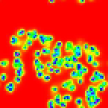
$k=0.08$	$k=0.07$	$k=0.06$	$k=0.05$	$k=0.04$	$k=0.03$

Figure 1: Reference patterns of the GS reaction-diffusion system subject to internal reaction noise. The initial condition was the uniform red, trivial state ($U=1,V=0$) with a small localized, perturbing pulse (see text for details). Concentration of field $U(x,y,t)$ is displayed at $t=5000$ for the parameter range $F=\nu=0.025$, $k=\mu-\nu=[0.025:0.08]$.

a	b	c
$F=0.0025$	$F=0.01$	$F=0.01$

Figure 2: The concentration of the field $U(x,y,t)$ displayed at $t=5000$ for (a) $F$=0.0025, $k=0.05$ (b) $F$=0.01, $k=0.05$ (c) $F$=0.01, $k=0.0375$. As $F$ is decreased the size of the structures in the patterns increases. The patterns are designated with the corresponding letter of the reference case in Fig. 1, which have a greater value of $F$. Notice that the size of the square region depicted in the figures is the same.

Figure 3: Parameter space diagram with $k=\mu-\nu$ and $F=\nu$. The letters indicate the location where similar patterns to the reference ones in Fig. (1) were found. A transitional pattern between two reference cases is designated by a pair of two corresponding letters (e.g., ed and cb). R indicates that the system evolved to the inactive uniform trivial, red, state. See the text for an explanation of the solid-line.

B	i	ii	c
$(F,k)=(0.05,0.055)$  $t=0$	$t=20$	$t=40$	$t=600$

B	I	II	a
$(F,k)=(0.05,0.0725)$  $t=0$	$t=40$	$t=50$	$t=3500$

Figure 4: Time evolution of the homogeneous initial condition ($U=0.3,V=0.25$): (B)-(i)-(ii)-(c) for $k=0.055$ and $F=0.05$, and (B)-(I)-(II)-(a) for $k=0.075$ and $F=0.05$.