Coulomb scattering in nitride based self-assembled quantum-dot systems

Abstract

We study the carrier capture and relaxation due to Coulomb scattering in group-III nitride quantum dots on the basis of population kinetics. For the states involved in the scattering processes the combined influence of the quantum-confined Stark effect and many-body renormalizations is taken into account. The charge separation induced by the built-in field has important consequences on the capture and relaxation rates. It is shown that its main effect comes through the renormalization of the energies of the states involved in the collisions, and leads to an increase in the scattering efficency.

I Introduction

In recent years, quantum dots (QDs) have emerged as a powerful tool to tailor the light-emission properties of semiconductors.Bimberg et al. (1998) Applications range from quantum dot lasers and ultrafast amplifiers to cavity-quantum electrodynamics and nonclassical light generation.Michler (2003) As a new material system, group-III nitrides are of intense current interest due to their extended range of emission frequencies from amber up to ultraviolet as well as their potential for high-power/high-temperature electronic devices.Nakamura (1998); Jain et al. (2000) While the nonradiative loss of carriers due to trapping at threading dislocations lowers the efficiency of group-III nitride quantum-well light emitters, this effect is reduced by the three-dimensional confinement in QDs.Damilano et al. (1999) Studies of the photoluminescence spectra Kalliakos et al. (2004) and dynamics Krestnikov et al. (2002); Oliver et al. (2003) are used to demonstrate and analyze efficient recombination processes from the localized QD states.

Extensive work has been done to study the electronic states in group-III nitrides.Vurgaftman and Meyer (2003) The valence-band structure has a strongly non-parabolic dispersion and a pronounced mass anisotropy. Chuang and Chang (1996) Nitride-based heterostructures with a wurtzite crystal structure are known to have strong built-in electrostatic fields due to spontaneous polarization and piezoelectric effects which have been analyzed in ab-initio electronic structure calculations Bernardini et al. (1997); Bernardini and Fiorentini (1998) and in comparison with photoluminescence experiments.Cingolani et al. (2000) Tight-binding calculations of QD states have been used to study free-carrier optical transitions.Ranjan et al. (2003)

While the aforementioned theoretical investigations are devoted to the single-particle states and transitions, it is known from GaAs-based QD systems, that the emission properties are strongly influenced by many-body effects. Self-organized QD systems, grown in the Stranski-Krastanov mode, exhibit a single-particle energy spectrum with discrete energies for localized states as well as a quasi-continuum of delocalized wetting layer (WL) states at higher energies. The carrier-carrier Coulomb interaction provides efficient scattering processes from the delocalized into the localized states (carrier capture) as well as fast transitions between localized states (carrier relaxation), which can be assisted by carriers in bound (QD) or extended (WL) states. The dependence of the scattering efficiency on the excitation conditions has been calculated for GaAs-based QDs on various levels of refinement.Bockelmann and Egeler (1992); Vurgaftman et al. (1994); Brasken et al. (1998); Magnusdottir et al. (2003); Nielsen et al. (2004) The scattering rates are of central importance for the photoluminescence as well as for the laser efficiency and dynamics. The same interaction processes also lead to a renormalization of the electronic states (resulting in line shifts for the optical transitions) as well as to dephasing (line broadening) effects, which directly determine absorption and gain spectra. Schneider et al. (2004)

With the current attention on nitride-based QDs the question raises, to which extent previous results are modified by the peculiarities of this material system. Specifically, we study how the strong electrostatic fields and the corresponding changes of the single-particle wave functions and energies influence the carrier-carrier scattering processes. For this purpose, we have to analyze the competing influence of the internal fields and of the many-body renormalizations. Since previous investigations of carrier-carrier scattering in semiconductor QDs have been performed for free-carrier energies entering the scattering integrals, an independent second purpose of this paper is the inclusion of self-consistently renormalized energies.

Renormalizations of the single-particle energies are due to direct electrostatic (Hartree) Coulomb interaction, exchange interaction, and screening. While these effects generally contribute due to possible charging of the QDs, in the considered wurtzite structure they are additionally modified by the presence of the built-in fields. In this paper we show that the discussed changes of the single-particle energies have a much stronger impact on the carrier scattering processes than modifications of the single-particle wave functions.

Many-body effects were also considered for the case of few excited carriers restricted to localized states of GaN-QD.De Rinaldis et al. (2004) In this regime, the emission properties reflect the multi-exciton states. In our paper, we are interested in kinetic processes for the opposite limit of high densities of carriers populating both QD and WL states (as typical for QD lasers).

For the evaluation of scattering processes, we use kinetic equations for the carrier occupation probabilities which include direct and exchange Coulomb interaction under the influence of carrier screening as well as population effects (Pauli-blocking) of the involved electronic states. Based on the single particle states and Coulomb interaction matrix elements, scattering processes are evaluated on the level of second-order Born approximation.Nielsen et al. (2004)

The paper is organized as follows. In Sec. II we summarize the main ingredients of our theory which include the kinetic equations, the single-particle states and their renormalization as well as the interaction matrix elements. Details regarding the WL states and screening effects are given in appendices. In Sec. III the QD model is described and the numerical results for energy renormalization and scattering times are presented.

II Theory for carrier-carrier Coulomb scattering

To analyze the role of carrier-carrier scattering in nitride-based QD systems, we use a kinetic equation with Boltzmann scattering integrals.Nielsen et al. (2004) The dynamics of the carrier population $f_{\nu}(t)$ in an arbitrary state $\nu$ is determined by in-scattering processes, weighted with the nonoccupation of this state, and by out-scattering processes, weighted with the occupation according to

$$\frac{\partial}{\partial t}\>f_{\nu} = (1-f_{\nu})S_{\nu}^{\text{in}}-f_{\nu}S_{\nu}^{\text{out}}.$$ (1)

The in-scattering rate is given by

$$S_{\nu}^{\text{in}} =\frac{2\pi}{\hbar}\sum\limits_{\nu_{1},\nu_{2},\nu_{3}}\>W_{\nu\nu_{2}\nu_{3}\nu_{1}}[W^{*}_{\nu\nu_{2}\nu_{3}\nu_{1}}-W^{*}_{\nu\nu_{2}\nu_{1}\nu_{3}}]$$

$$\times\big{\{}f_{\nu_{1}}(1-f_{\nu_{2}})f_{\nu_{3}}\delta(\widetilde{\varepsilon}_{\nu}-\widetilde{\varepsilon}_{\nu_{1}}+\widetilde{\varepsilon}_{\nu_{2}}-\widetilde{\varepsilon}_{\nu_{3}})\big{\}},$$ (2)

where the first and second term in the square brackets correspond to direct and exchange Coulomb scattering, respectively. The matrix elements of the screened Coulomb interaction, $W_{\nu\nu_{2}\nu_{3}\nu_{1}}$, are calculated in Section II.2. The delta-function describes energy conservation in the Markov limit. Single-particle energies $\widetilde{\varepsilon}_{\nu}$ of state $\nu$ are renormalized by the Coulomb interaction as discussed in Sections II.4 and II.5. A similar expression for the out-scattering rate $S_{\nu}^{\text{out}}$ is obtained by replacing $f\rightarrow 1-f$.

Scattering processes described by Eqs. (1) and (2) conserve the total energy and separately the electron and hole numbers. As a result, the combined action of the discussed scattering processes will evolve the distribution functions of electrons and holes towards Fermi-Dirac functions with common temperature where the QD and WL electrons (holes) will have the same chemical potential $\mu_{e}$ ($\mu_{h}$). During such a time evolution towards quasi-equilibrium the relative importance of various scattering processes is expected to change via their dependence on the (non-equilibrium) carrier distribution functions for WL and QD states. A direct measure for the efficiency of various scattering processes can be given in the relaxation-time approximation Nielsen et al. (2004) where one calculates the characteristic time on which a small perturbation of the system from thermal equilibrium is obliterated. We use this method to investigate the influence of the built-in electrostatic field in nitride-based QDs on the carrier-density dependent scattering efficiency.

II.1 Quantum-dot model system

Recent progress in tight-binding and ${\bf k}\cdot{\bf p}$ models has been made in calculating QD electronic single-particle states including the confinement geometry, strain and built-in electrostatic field effects. The special features of the wurtzite QD structures have been addressed in Refs. [Ranjan et al., 2003; Andreev and O’Reilly, 2000; Bagga et al., 2003; Fonoberov and Balandin, 2003], while zinc-blende QD structures have been studied in Refs. [Bagga et al., 2003; Fonoberov and Balandin, 2003; Sheng et al., 2005; Williamson et al., 2000; Bester and Zunger, 2005; Schulz and Czycholl, 2005]. Our goals differ from these investigations in the respect that, for given single-particle states and energies, we need to determine Coulomb interaction matrix elements in order to calculate many-body energy renormalizations and scattering processes. For this purpose we choose a simple representation of wave functions for lens-shaped quantum dots Wojs et al. (1996) which allows to separate the in-plane motion (with weak confinement for the states localized at the QD position and without confinement for the states delocalized over the WL plane) from the motion in growth direction with strong confinement. This leads to the ansatz

$$\Phi_{\nu}({\bf r})=\varphi_{l}^{b}({\bm{\varrho}})\;\xi_{\sigma}^{b}(z)\;u_{b}({\bf r})$$ (3)

where the WL extends in the plane described by $\bm{\varrho}=(x,y)$. $\varphi$ and $\xi$ are the envelope functions in this plane and in the perpendicular growth direction, respectively, and $u$ are Bloch functions. $\nu$ represents a set of quantum numbers with $l$ for the in-plane component (including the spin), $\sigma$ for the $z$-direction, and $b$ is the band index. In the following we consider an ensemble of randomly distributed identical QDs with non-overlapping localized states. The total number of QDs, $N$, leads in the large area limit to a constant QD density $n_{\text{QD}}=\lim_{A\rightarrow\infty}N/A$.

Regarding the dependence of the results on the choice of wave functions, we find that not so much the particular form but rather the correct symmetry is of relevance. Even tough a more accurate treatment is expected to mix the in-plane and $z$-coordinates, the ansatz (3) is preserving the symmetry.

II.2 Coulomb matrix elements

The interaction matrix elements of the bare Coulomb potential $v({\bf r}-{\bf r^{\prime}})=e^{2}/(4\pi\varepsilon_{0}\epsilon|{\bf r}-{\bf r^{\prime}}|)$ with the background dielectric function $\epsilon$ are given by

$$V_{\nu\nu_{2}\nu_{3}\nu_{1}} =\int d^{3}r\;d^{3}r^{\prime}\;$$

$$\Phi^{*}_{\nu}({\bf r})\Phi^{*}_{\nu_{2}}({\bf r^{\prime}})v({\bf r}-{\bf r^{\prime}})\Phi_{\nu_{3}}({\bf r^{\prime}})\Phi_{\nu_{1}}({\bf r}).$$ (4)

This expression is further specified with the help of Eq. (3), the Fourier transform of the Coulomb potential, and by introducing the in-plane Coulomb matrix elements with the two-dimensional momentum ${\bf q}$,

$$V_{\sigma\sigma_{2}\sigma_{3}\sigma_{1}}^{b,b^{\prime}}({\bf q}) =\frac{e^{2}}{2\varepsilon_{0}\epsilon\,q}\int dz\;dz^{\prime}\;$$

$$\xi_{\sigma}^{b}(z)^{*}\xi_{\sigma_{2}}^{b^{\prime}}(z^{\prime})^{*}e^{-q|z-z^{\prime}|}\xi_{\sigma_{3}}^{b^{\prime}}(z^{\prime})\xi_{\sigma_{1}}^{b}(z).$$ (5)

Limiting the calculations to the first bound state of the strong confinement problem (in $z$-direction), all the $\sigma$ indices above take only one value and will be dropped in what follows. Also, the band indices associated with $\nu_{1}$ and $\nu_{3}$ are the same as those of $\nu$ and $\nu_{2}$, respectively, so that only two of them have to be specified. Therefore Eq. (4) reads

$$V_{l,l_{2},l_{3},l_{1}}^{b,b_{2}} = \frac{1}{A}\>\sum\limits_{\bf q}\,V^{b,b_{2}}({\bf q})\,$$ (6)

$$\times\int d^{2}\varrho\>\varphi_{l}^{b}({\bm{\varrho}})^{*}\varphi_{l_{1}}^{b}({\bm{\varrho}})\>e^{-i{\bf q}\cdot{\bm{\varrho}}}\;$$

$$\times\int d^{2}\varrho^{\prime}\>\varphi_{l_{2}}^{b_{2}}({\bm{\varrho}}^{\prime})^{*}\varphi_{l_{3}}^{b_{2}}({\bm{\varrho}}^{\prime})\>e^{i{\bf q}\cdot{\bm{\varrho}}^{\prime}}.$$

The obtained separation of integrals over in-plane and $z$-components greatly simplifies the computational effort. For practical calculations we use solutions of a two-dimensional harmonic potential for the in-plane wave functions of the localized states and orthogonalized plane wave (OPW) solutions, discussed in Appendix A, for the in-plane components of the delocalized states. Then the in-plane integrals in Eq. (6) can be determined to a large extent analytically for all possible combinations of QD and WL states. The calculation of the wave functions in growth direction, which is used to evaluate the in-plane Coulomb matrix elements, Eq. (5), is outlined in the next section. Screened Coulomb matrix elements are obtained from Eqs. (5) and (6) according to the procedure described in detail in Ref. [Nielsen et al., 2004].

II.3 Quantum-confined Stark effect

To account for the built-in electrostatic fields of the wurtzite structure in the growth-direction, which gives rise to the quantum-confined Stark effect, we solve the one-dimensional Schrödinger equation Chow et al. (1999); Chow and Koch (1999)

$$\left[-\frac{\hbar^{2}}{2m_{b}}\frac{\partial^{2}}{\partial z^{2}}+U^{b}(z)\right]\xi^{b}(z)=E_{b}(z)\xi^{b}(z),$$ (7)

where the potential

$$U^{b}(z)=U_{0}^{b}(z)+U_{\text{p}}^{b}(z)+U_{\text{scr}}^{b}(z),$$ (8)

consists of the bare confinement potential in $z$-direction, $U_{0}^{b}(z)$, as well as the intrinsic electrical and screening fields, $U_{\text{p}}^{b}(z)$ and $U_{\text{scr}}^{b}(z)$, respectively. The latter is the electrostatic field due to the separation of electron and hole wave functions by the built-in field. Following Ref. [Chow and Koch, 1999] we calculate the corresponding screening potential from a solution of the Poisson equation for a set of uniformly charged sheets according to

$$U_{\text{scr}}^{e,h}(z)=\frac{\mp e^{2}N_{\text{sys}}}{2\varepsilon_{0}\epsilon}\int\mathrm{d}z^{\prime}\left[|\xi^{e}(z^{\prime})|^{2}-|\xi^{h}(z^{\prime})|^{2}\right]|z-z^{\prime}|.$$ (9)

Equations (7)-(9) have to be evaluated selfconsistently for a given total (QD plus WL) carrier density $N_{\text{sys}}$ in the system.

II.4 Hartree-Fock energy renormalization

The Hartree-Fock (HF) contribution to the energy renormalization of an arbitrary state $\nu$ (QD or WL) is given by

$$\widetilde{\varepsilon}_{\nu} = \varepsilon_{\nu}+\Delta^{\text{HF}}_{\nu},$$ (10)

where $\varepsilon_{\nu}$ is the free-carrier energy and the HF shift follows from

$$\Delta^{\text{HF}}_{\nu} = \Delta^{\text{H}}_{\nu}+\Delta^{\text{F}}_{\nu}$$

$$= \sum_{\nu^{\prime}}\left[V_{\nu\nu^{\prime}\nu^{\prime}\nu}-V_{\nu\nu^{\prime}\nu\nu^{\prime}}\right]f_{\nu^{\prime}}.$$

The first part corresponds to the Hartree (direct) term and the second part is the Fock (exchange) contribution. The equation is written in a general basis. For a system with local charge neutrality, like bulk semiconductors or quantum wells, the Hartree term vanishes while the Fock term leads to an energy reduction as used, e.g., in the semiconductor Bloch equations.Haug and Koch (1994)

For the QD and OPW-WL states discussed in this paper, the absence of local charge neutrality leads to Hartree terms which are evaluated in Appendix B. Regarding the quantum numbers, introduced in Section II.1, we further specify the following notation: For the in-plane envelopes we use the two-dimensional momentum ${\bf k}$ for the delocalized WL states and $\alpha=(m,{\bf R})$ for the localized QD states, where ${\bf R}$ is the QD position and the discrete quantum numbers for a particular QD are collected in $m$. The spin index is tacitly included in either $m$ or ${\bf k}$.

Following Appendix B, we find that the Hartree shifts of the WL states vanish due to compensating contributions from QD and WL carriers,

$$\Delta^{\text{H}}_{b,{\bf k}} = 0.$$ (12)

For a random distribution of QDs this is related to the spatial homogeneity restored on a global length scale and to the global charge neutrality of the system. For the same reason, the Hartree shift of a localized QD state is only provided by states from the same QD while Hartree shifts due to carriers in other QD and WL states compensate each other,

$$\Delta^{\text{H}}_{b,m} = \sum_{b^{\prime},m^{\prime}}\;V_{mm^{\prime}m^{\prime}m}^{b,b^{\prime}}\;f^{b^{\prime}}_{m^{\prime}}\,.$$ (13)

From electrostatics one expects the same result, provided that the WL is modeled as a constant area charge of opposite sign to the QD total charge. Then the constant part of the Fourier expansion of the Coulomb matrix elements in Eq. (6), i.e. the ${\bf q}=0$ contribution, for the QDs balances the constant area charge from the WL.

On the other hand, since $\Delta^{\text{H}}_{b,m}$ probes the local charge density at the site of the QD due to the contributions of QD and WL carriers, one expects an influence of the WL on the QD Hartree energy shift. Locally on the QD length scale, the WL states are not homogeneous as a result of the QD presence. This causes a departure from the picture where the WL states contribute only in an averaged manner (via the ${\bf q}=0$ term). Intuitively, one would expect that an increasing amount of carriers in the WL will start to screen the Coulomb interaction between the QD carriers. Following this picture we therefore replace the bare Coulomb potential with the screened one in Eq. (13), i.e., $\Delta^{\text{H}}_{b,m}\rightarrow\Delta^{\text{SH}}_{b,m}$. In Appendices  B and  C more support is given to this argumentation.

In the exchange terms, the summation over the QD positions can be performed directly, since the associated QD phase factors disappear for the Coulomb matrix elements $V_{mm^{\prime}mm^{\prime}}$ and $V_{\alpha{\bf k}\alpha{\bf k}}$ as seen from Eq. (20) and Eq. (21), respectively. The resulting exchange energy shifts contain the QD and WL contributions,

$$\Delta^{\text{F}}_{b,m}= - \sum_{m^{\prime}}\;V_{mm^{\prime}mm^{\prime}}^{b,b}\,f^{b}_{m^{\prime}}$$ (14)

$$- \sum_{{\bf k}^{\prime}}\;V_{m{\bf k}^{\prime}m{\bf k}^{\prime}}^{b,b}\,f^{b}_{{\bf k}^{\prime}},$$

$$\Delta^{\text{F}}_{b,{\bf k}}= - N\cdot\sum_{m^{\prime}}\;V_{{\bf k}m^{\prime}{\bf k}m^{\prime}}^{b,b}\,f^{b}_{m^{\prime}}$$ (15)

$$- \sum_{{\bf k}^{\prime}}\;V_{{\bf k}{\bf k}^{\prime}{\bf k}{\bf k}^{\prime}}^{b,b}\,f^{b}_{{\bf k}^{\prime}}.$$

Since there is an area associated with the Coulomb matrix element $V_{{\bf k}m^{\prime}{\bf k}m^{\prime}}$, the QD density $n_{\text{QD}}=N/A$ enters in Eq. (15).

II.5 Screened exchange and Coulomb hole

The HF Coulomb interaction provides only the first approximation for energy renormalizations; correlation contributions can lead to important corrections. A frequently used extension of the HF energy shifts for high-density plasma excitation is the screened-exchange and Coulomb-hole approximation.Haug and Koch (1994) On this level, the combined contributions of Coulomb exchange interaction and Coulomb correlations beyond HF to the energy renormalizations are approximated with the screened exchange term (where the bare Coulomb potential in the Fock term is replaced by a screened one) plus an energy shift denoted as Coulomb-hole contribution. The Coulomb hole self-energy reads Haug and Koch (1994)

$$\Sigma^{\text{CH}}({\bf r}_{1},{\bf r}_{2},t_{1},t_{2}) =\frac{1}{2}\delta({\bf r}_{1}-{\bf r}_{2})\delta(t_{1}-t_{2})$$

$$\times\left[W({\bf r}_{1},{\bf r}_{2},t_{1})-V({\bf r}_{1}-{\bf r}_{2})\right],$$ (16)

with the statically screened Coulomb potential $W$. In a general eigenfunction basis, this leads to the Coulomb-hole energy shift

$$\Delta^{\text{CH}}_{\nu}(t) =\frac{1}{2}\sum_{\nu^{\prime}}\left[W_{\nu\nu^{\prime}\nu\nu^{\prime}}(t)-V_{\nu\nu^{\prime}\nu\nu^{\prime}}\right].$$ (17)

In Eqs. (14) and (15) we therefore replace the bare Coulomb potential with the screened one and substitute the Fock energy shift with the screened exchange plus the Coulomb hole, $\Delta^{\text{F}}_{\nu}\rightarrow\Delta^{\text{SX}}_{\nu}$ + $\Delta^{\text{CH}}_{\nu}$. In the limit of low carrier densities, the screened Coulomb potential reduces to the bare one, the Coulomb hole vanishes, and we recover the HF result.

III Results

We start this Section by describing the model we use and the material parameters employed for calculating the one-particle states. These correspond to the unexcited system. The next step is to renormalize these states in a self-consistent way to include the influence of the carrier population and the presence of the built-in field, as described in Section  II. These single-particle properties enter the scattering integrals, Eq. (2).

For the discussion of the numerical results one should bear in mind the two main consequences of the built-in field. On the one hand, the self-consistent energies entering the Fermi functions and the energy-conservation are sensitive to the electron-hole separation induced by the built-in electrostatic field. On the other hand, the Coulomb matrix elements are changed due to modifications in the wave-function shapes and overlapping.

III.1 The model and its parameters

Table 1: Material parameters used in the calculations.

Parameter		GaN		InN		In0.2Ga0.8N
$E_{g}$[300 K] (eV)		3.438		0.756		2.677
$\Delta E_{e}$ (eV)						0.457
$\Delta E_{h}$ (eV)						0.304
$\epsilon$		8.9		15.3		10.2
$m_{e}$ ($m_{0}$)		0.2		0.07		0.174
$A_{1}$		-7.21		-8.21		-7.41
$A_{2}$		-0.44		-0.68		-0.488
$A_{3}$		6.68		7.57		6.858
$A_{4}$		-3.46		-5.23		-3.814
$A_{5}$		-3.40		-5.11		-3.742
$\Delta_{\text{so}}$ (eV)		0.017		0.005		0.0146
Quantum well (nm)						3.0
$F_{\text{QD-WL}}$ (MV/cm)						1.5
$F_{\text{barrier}}$ (MV/cm)						0.75

In the following examples we consider an InGaN/GaN QD-WL system using typical InGaN parameters Vurgaftman and Meyer (2003) listed in Table 1. For the alloy, we have interpolated linearly the dielectric constant $\epsilon$, the isotropic electron mass $m_{e}$, the hole mass parameters $A_{i}$ and the spin-orbit splitting $\Delta_{\text{so}}$.

A specific feature of the wurtzite structure nitrides is the strong mass anisotropy of the holes. The mass of the heavy hole (HH) in the $z$-direction, is given by $m^{\ast}_{z}=m_{0}/|A_{1}+A_{3}|$ with the free electron mass $m_{0}$ and the mass parameters $A_{1}$ and $A_{3}$.Chuang and Chang (1996) For the in-plane motion, a strong hybridization between the HH and the light-hole (LH) subband leads to nonparabolic bands. This is due to the fact that the small HH-LH splitting, induced by the spin-orbit interaction, is enhanced by neither the strain nor the $z$-confinement. To include the hybridization effect we use a nonparabolic HH dispersion,Chuang and Chang (1996)

$$\varepsilon_{{\bf k}}^{h} =-\alpha(A_{2}+A_{4}){\bf k}^{2}-\sqrt{\Delta_{2}^{2}+\alpha^{2}A^{2}_{5}{\bf k}^{4}},$$ (18)

where $\alpha=\hbar^{2}/2m_{0}$ and $\Delta_{2}=\Delta_{\text{so}}/3$. For the motion of the electrons, isotropic effective mass and parabolic dispersion are considered. Conduction ($\Delta E_{e}$) and valence ($\Delta E_{h}$) band offsets for InGaN grown on GaN have been estimated by splitting the gap energy difference between bulk GaN and the alloy with a band offset ratio 60:40 for electrons and holes, according to Refs. [Wu and Walukiewicz, 2003; Zang et al., 2004].

Compared to usual zinc-blende structure, the wurtzite structure is characterized by large built-in electric fields. The strength of the fields is related to the spontaneous polarization discontinuity at the heterojunction interfaces and the piezoelectric polarization.Bernardini et al. (1997); Bernardini and Fiorentini (1998) Internal fields in InGaN/GaN heterojunctions of a few MV/cm have been reported,Lai et al. (2002); Zang et al. (2004) typically in a sawtooth profile, where the field in the QD-WL system has a different magnitude and opposite direction to the field of the barrier (reflecting a set of capacitors with non-equal surface charges). For the field inside the QD-WL region and in the barrier, we consider $F_{\text{QD-WL}}=1.5$ MV/cm and $F_{\text{barrier}}=0.75$ MV/cm, respectively.

Table 2: QD parameters used in the calculations.

Parameter		Electrons		Holes
Shells		s, p		s, p, d
Level spacing (meV)		90.0		30.0
$\varepsilon_{\text{s}}$ (meV)		-160.0		-80.0
$\varepsilon_{\text{p}}$ (meV)		-70.0		-50.0
$\varepsilon_{\text{d}}$ (meV)				-20.0
QD density (cm-2)						$10^{10}$

As the estimated effective hole masses Chuang and Chang (1996) are larger than the electron mass, we expect the QD’s to confine more states for holes than for electrons. On the same basis, the level spacing which scales inversely with the mass, is larger for electrons than for holes. The in-plane QD confinement is modeled with a 2D parabolic potential, capable of binding two energy shells (s and p) for electrons and three (s,p,d) for holes. The degeneracies of these shells (apart from spin) are $1,2$ and $3$ for s,p and d, respectively. For electrons we assume a level spacing of 90 meV with the p-shell 70 meV below the WL continuum edge, while for holes we assume a level spacing of 30 meV with the d-shell 20 meV below the WL continuum edge. Thus the $e_{s}-h_{s}$ QD transition is close to the range given in Ref. [Oliver et al., 2003; Lin et al., 2002]. The QD parameters are summarized in Table 2. Finally, we assume $z$-direction confinement wave functions which are band dependent but equal for QD and WL states.Nielsen et al. (2004)

The harmonic oscillator (HO) inverse localization length $\beta$ is deduced from the level spacing via $\hbar\omega_{\text{HO}}=\hbar^{2}\beta^{2}/m^{\ast}$. For electrons the effective mass of Table 1 is taken. For holes we use the mass resulting from Eq. (18) in the small $k$ limit, $m^{\ast}_{h}=m_{0}/|A_{2}+A_{4}|$. This is justified by the typical QD diameters of 100Å  - 200Å , which correspond to the region around $k=0$ where the first term of Eq. (18) is dominant.

III.2 Schrödinger and Poisson equations

The charge separation of carriers along the growth direction $z$ under the influence of the built-in electrostatic fields, obtained from a self-consistent solution of Eqs. (7)-(9) is shown in Fig. 1 (a) and (b). A clear overlap reduction of the wave functions for electrons and holes is observed. This leads to a decreasing form factor (the double integral in Eq. (5) which modifies the 2D Fourier transform of the Coulomb interaction) for the electron-hole interaction while the stronger carrier localization increases the form factors for electron-electron and hole-hole interaction. Thus, the presence of the built-in field leads to an effective reduction of the electron-hole interaction, while the electron-electron and the hole-hole interaction is enhanced. The screening field turns out to be a small correction to the strong built-in field for the range of densities considered.

Figure 1: Total confinement potential $U(z)$ (solid line) and modulus amplitude of the $z$-component wave function $|\xi(z)|^{2}$ (dashed line) along the growth direction $z$ for electrons (a) and holes (b) in the presence of the built-in field at a total carrier density $N_{\text{sys}}=10^{10}$ cm^-2. The dotted lines are the wave function amplitudes for zero field.

III.3 Renormalized energies

Figure 2: Renormalized energies as a function of the total carrier density in system $N_{\text{sys}}$ for s-shell (solid lines), p-shell (dotted lines), d_±-shell (dashed lines), and WL ${\bf k}=0$ (dashed-dotted lines). Calculation with (a),(c) and without (b),(d) electrostatic field are shown for electrons (a),(b) and holes (c),(d). The temperature is 300 K.

For a total carrier density $N_{\text{sys}}$, the corresponding carrier distributions $f_{\nu}$ in thermal equilibrium are used to determine the renormalized energies from the self-consistent solution of the equation $\widetilde{\varepsilon}_{\nu}=\varepsilon_{\nu}+\Delta_{\nu}^{\text{SH}}+\Delta_{\nu}^{\text{SX}}+\Delta_{\nu}^{\text{CH}}$, for the QD and WL states. For $\varepsilon_{\nu}$ we use the energies listed in Table 2 for the QD bound states and the dispersion law of Eq. (18) for the WL hole states.

The density dependence of the renormalized electron and hole energies is shown in Fig. 2 (a) and (c), respectively, in the presence of the built-in field. The corresponding results without the built-in field are given in Fig. 2 (b) and (d) for comparison. The renormalized d-shell is split into two degenerate d_± states and a d₀ state, with a separation of a few meV.

Quantitatively, the QD levels experience a smaller energy shift for the built-in field compared to the zero field case. The origin of this difference lies in the Hartree term, which reflects the electrostatic interaction of a given carrier with all the others. The field-induced change of the $z$-confinement functions tends to separate the electrons from the holes and, as a consequence for both, the repulsive part of the Hartree term is increased and the attractive part is decreased. This effect is illustrated explicitly in Fig. 3 for the p-shell where the four different contributions to the renormalized energies are shown. For electrons the Hartree shift is repulsive both in the presence and in the absence of the built-in field, but more so in the former case. For holes, the built-in field makes the Hartree term less attractive. In both cases the net result is a set of shallower bound states. For the sake of completeness we mention that the different sign of the Hartree field for electrons and holes comes from the difference in the QD population of electrons and holes and from the band dependence of the Coulomb matrix elements.

The screened exchange and Coulomb hole terms are not significantly different for with and without built-in field. As the extended WL states are only renormalized by the screened exchange and Coulomb hole term, we find an overall negative energy shift, lowering the free spectrum by an almost ${\bf k}$-independent shift (not shown).

Figure 3: Same as Fig. 2 for different contributions to the renormalized p-shell energy $\widetilde{\varepsilon}_{\text{p}}$ which are the free energy $\varepsilon_{\text{p}}$ (dashed dotted line), screened Hartree shift $\Delta_{\text{p}}^{\text{SH}}$ (dotted line), screened exchange shift $\Delta_{\text{p}}^{\text{SX}}$ (solid line), and Coulomb hole shift $\Delta^{\text{CH}}_{\text{p}}$ (dashed line).

III.4 Capture and relaxation times

To quantify the importance of the different scattering processes, we study their dependence on the total carrier density in thermal equilibrium. Using the relaxation time approximation Nielsen et al. (2004) one can introduce a scattering time $\tau_{\nu}$ for a given process according to

$$\tau_{\nu} = \left[S_{\nu}^{\text{in}}+S_{\nu}^{\text{out}}\right]^{-1},$$ (19)

which gives a characteristic time on which the system will return to its thermal equilibrium distribution if exposed to a small perturbation, i.e., $\dot{f}_{\nu}=-(f_{\nu}-F_{\nu})/\tau_{\nu}$, with $F_{\nu}$ being the thermal equilibrium distribution.

The scattering times are changed by the built-in field through different competing mechanisms. On the one hand the matrix elements are modified (see Section III.2), on the other hand the QD energies are pushed closer to the WL continuum (Section III.3).

For illustrative purposes, we first study the influence of the built-in field on the scattering times by using the free (unrenormalized) energies within the scattering integrals. This reveals the field effect solely on the Coulomb matrix elements via the wave-function changes. As an example we consider a capture process, where an electron or hole from the WL is scattered into the QD while another WL carrier (electron or hole) is scattered to an energetically higher WL state, as well as the reverse process. (Both contribute to the scattering time according to the relaxation-time approximation.) Thus the outer index in Eq. (1) is a QD state while the three summation indices in Eq. (2) belong to the WL states for this example shown in Figure 4.

First we discuss the density dependence. The capture time decreases with increasing carrier density, as more scattering partners become available. Furthermore, capture times for electrons are slower than for holes, because the QD electron levels are placed energetically deeper below the WL continuum edge. For energy-conserving scattering processes, the excess energy of a WL electron which is captured to the QD must be transferred to another carrier from the WL in the present example. In this way a capture to an energetically deep lying QD state is associated with large momentum transfer for the WL carriers. As the matrix elements have a Gaussian dependence on the in-plane momentum, scattering to WL states with high momentum is suppressed.

Figure 4: Capture times for the p-shell as a function of the total carrier density in the system $N_{\text{sys}}$ using the free (unrenormalized energies), with (solid lines) and without (dotted lines) built-in electrostatic field.

The changes in the capture times produced by the field in the case of unrenormalized energies are minimal. This proves that the competing trends described in Section III.2 are nearly compensating each other, with a slight dominance of the effect of electron-hole scattering reduction.

Figure 5: Capture times as a function of the total carrier density in the system $N_{\text{sys}}$ for s-shell (solid lines), p-shell (dotted lines), d₀-shell (dashed-dotted lines), and d_±-shell (dashed lines).

For the calculation of the capture times in Fig. 5, based on WL assisted capture processes,Nielsen et al. (2004) the renormalized energies are included in the scattering integrals $S_{\nu}^{\text{in,out}}$. Now the capture times become substantially shorter in the presence of the built-in field compared to the zero field case. Thus, the energy separation of the QD levels from the WL edge plays now the dominant role in the scattering times. Even though for the built-in field, the capture processes are somewhat slowed down by the reduction of the electron-hole interaction, they are still faster compared to the zero field case, where due to the electron-hole interaction the QD levels are energetically deeper in the QD.

Figure 6 shows the WL assisted QD relaxation times for processes where a QD electron (hole) scatters to a different QD electron (hole) state by means of a WL carrier. Alternatively, a QD carrier performs a transition to the WL while another WL carrier scatters into a different QD state.Nielsen et al. (2004) Thus the outer index in Eq. (1) belongs to a QD state while two of the summation indices in Eq. (2) correspond to WL states and one label to a QD state. Mixed QD relaxation processes,Nielsen et al. (2004) where e.g. a QD electron scatters out to the WL while another hole from the WL scatters down to the QD hole state play only a minor role due to the charge separation of the electrons and holes caused by the built-in field.

Figure 6: Relaxation times as a function of the total carrier density in the system $N_{\text{sys}}$ with labeling as in Fig. 5.

Generally, the relaxation times for holes are one or two orders of magnitude shorter than for electrons, since the QD energy level spacing is larger for the latter. With built-in field the relaxation times become shorter compared to the zero field case, where the QD energy level spacing is larger (with the exception of a slightly slower relaxation of the s-shell electrons). Relaxation times for scattering between QD states are in general more than one order of magnitude shorter than capture. For the p-shell electron relaxation, a saturation effect due to Pauli blocking is observed at higher densities, which leads to comparable capture and relaxation times.

IV Conclusion

The presence of the built-in electrostatic field in wurtzite heterostructures causes a charge separation of electrons and holes along the growth direction, which in turn reduces the electron-hole interaction and increases the electron-electron and hole-hole interaction.

Our results show that the usually discussed importance of this effect on the interaction matrix elements only weakly influences the scattering rates. It turns out that the change of the self-consistently renormalized energies due to charge separation leads to a much stronger modification of the scattering rates. Specifically, for the influence on the interaction matrix elements, the reduction of electron-hole scattering is partly compensated by the increase of electron-electron and hole-hole scattering. In contrast, for the energy renormalization, the charge separation leads to increased repulsion and decreased attraction in the Hartree terms, both effects working in the same direction of shallower confined levels. This in turn causes an enhancement of the scattering efficiency.

As expected for the QD-WL system, the rates for carrier capture and relaxation strongly depend on the density of excited carriers in the localized and delocalized states. For intermediate densities, the scattering efficiency increases with carrier density. For large densities, Pauli-blocking and screening of the interaction matrix elements slow down a further increase of the scattering rates. For typical InGaN QD parameters, a QD density of 10¹⁰ cm^-2 and a carrier density of 10¹¹ cm^-2 at room temperature, direct capture of electrons (holes) to excited QD states results in scattering times on the order of 100 (10) ps. Relaxation times for scattering between the QD hole states are more than one order of magnitude shorter than capture, while at elevated densities the electron p-shell relaxation is of the same order of magnitude as capture.

Appendix A OPW states and interaction matrix elements

The basic idea of the following scheme is to construct an approximate single-particle basis for the combined QD-WL system which provides a feasible way to compute the interaction matrix elements, Eq. (4). We start from localized QD states $\varphi_{\alpha}$, as introduced in Sections II.1 and II.4 with $\alpha=(m,{\bf R})$, and WL states in the absence of QDs, which are assumed to have plane-wave envelope functions $\varphi_{\bf k}^{0}({\bm{\varrho}})=1/\sqrt{A}\,e^{i{\bf k}\cdot{\bm{\varrho}}}$ in the WL plane with the two-dimensional carrier momentum ${\bf k}$. Quantum numbers for spin, band index, and confinement in $z$-direction are not explicitly written for notational simplicity. In the presence of the QDs the orthogonality condition of the basis is imposed by projecting the plane waves on the subspace orthogonal to the QD states, as outlined in Ref. [Nielsen et al., 2004]. The WL states are therefore given by the OPW functions $|\varphi_{\bf k}\rangle=\frac{1}{N_{\bf k}}\>(|\varphi_{\bf k}^{0}\rangle-\sum_{\alpha}|\varphi_{\alpha}\rangle\langle\varphi_{\alpha}\>|\varphi_{\bf k}^{0}\rangle)$. Assuming QDs with nonoverlapping wave functions, the sum over $\alpha=(m,{\bf R})$ counts various QD states $m$ at different QD positions ${\bf R}$. For randomly distributed identical QDs, the normalization is given by $N_{\bf k}^{2}=1-N\sum_{m}|\langle\varphi_{m}|\varphi_{\bf k}^{0}\rangle|^{2}$.

This scheme allows to evaluate the in-plane integrals $\left\langle\nu|e^{i{\bf q}\cdot{\bm{\varrho}}}|\nu^{\prime}\right\rangle=\int\mathrm{d}^{2}\varrho\;\varphi_{\nu}^{\ast}({\bm{\varrho}})e^{i{\bf q}\cdot{\bm{\varrho}}}\varphi_{\nu^{\prime}}({\bm{\varrho}})$ which appear in the Coulomb matrix elements, Eq. (6), for various combinations of QD and WL states. When $\nu$ and $\nu^{\prime}$ are two QD states, one obtains

$$\left\langle\;\alpha\;|e^{i{\bf q}\cdot{\bm{\varrho}}}|\;\alpha^{\prime}\;\right\rangle =\left\langle\;m\;|e^{i{\bf q}\cdot{\bm{\varrho}}}|\;m^{\prime}\;\right\rangle\;e^{i{\bf q}\cdot{\bf R}}\;\delta_{{\bf R},{\bf R}^{\prime}}\,,$$ (20)

with the QD positions ${\bf R}$ and ${\bf R}^{\prime}$. For combinations of QD and WL states, one finds

$$\left\langle\;\alpha\;|e^{i{\bf q}\cdot{\bm{\varrho}}}|\;\varphi_{{\bf k}^{\prime}}\;\right\rangle =\left\langle\;m\;|e^{i{\bf q}\cdot{\bm{\varrho}}}|\;\varphi_{{\bf k}^{\prime}}\;\right\rangle\;e^{i({\bf k}^{\prime}+{\bf q})\cdot{\bf R}}\,,$$ (21)

and for two WL states

$$\left\langle\;\varphi_{\bf k}\;|e^{i{\bf q}\cdot{\bm{\varrho}}}|\;\varphi_{{\bf k}^{\prime}}\;\right\rangle =\delta_{{\bf k},\,{\bf q}+{\bf k}^{\prime}}\;D_{\text{OPW}}({\bf k},{\bf k}^{\prime},{\bf q})\,,$$ (22)

follows with

$$D_{\text{OPW}} ({\bf k},{\bf k}^{\prime},{\bf q})=\frac{1}{N_{{\bf k}}N_{{\bf k}^{\prime}}}$$ (23)

$$\times [1-N\sum\limits_{m}|\langle\varphi_{\bf k}^{0}|\varphi_{m}\rangle|^{2}-N\sum\limits_{m}|\langle\varphi_{m}|\varphi_{{\bf k}^{\prime}}^{0}\rangle|^{2}$$

$$+N\sum\limits_{m,m^{\prime}}\langle\varphi_{\bf k}^{0}|\varphi_{m}\rangle\langle\varphi_{m}|e^{i{\bf q}\cdot{\bm{\varrho}}}|\varphi_{m^{\prime}}\rangle\langle\varphi_{m^{\prime}}|\varphi_{{\bf k}^{\prime}}^{0}\rangle].$$

The orthogonality requirement of the wave functions is directly reflected in the interaction vertices $\left\langle\nu_{1}|e^{+i{\bf q}\cdot{\bm{\varrho}}}|\nu_{2}\right\rangle=\delta_{\nu_{1},\nu_{2}}$ for ${\bf q}=0$. Meaningful results for the interaction matrix elements can be expected only when the approximate model shows the same behavior. Since we start from orthogonal QD states at a given QD position and assume nonoverlapping wave functions for different QDs, Eq. (20) reduces to a Kronecker delta for ${\bf q}=0$. QD and OPW-WL states are orthogonal by construction, i.e., the requirement is also fulfilled for Eq. (21). As described in Ref. [Nielsen et al., 2004], it is the assumption of randomly distributed QDs which, in the large-area limit restores - on average - translational invariance and provides mutually orthogonal OPW states such that the above requirement is also obeyed by Eq. (22). Note that $D_{\text{OPW}}({\bf k},{\bf k},0)=1$.

Appendix B Hartree energy renormalization

Starting from Eq. (II.4), the Hartree energy shift of the QD states has contributions form the QD and from the WL carriers,

$$\Delta^{\text{H}}_{b,\alpha} =\sum_{b^{\prime},\alpha^{\prime}}V^{b,b^{\prime}}_{\alpha\alpha^{\prime}\alpha^{\prime}\alpha}\;f^{b^{\prime}}_{\alpha^{\prime}}+\sum_{b^{\prime},{\bf k}^{\prime}}V^{b,b^{\prime}}_{\alpha{\bf k}^{\prime}{\bf k}^{\prime}\alpha}\;f^{b^{\prime}}_{{\bf k}^{\prime}}$$

$$=\Delta^{\text{H},\text{QD}}_{b,\alpha}+\Delta^{\text{H},\text{WL}}_{b,\alpha}\;.$$ (24)

The QD contribution can be specified further using the notation introduced above and Eq. (6),

$$\Delta^{\text{H},\text{QD}}_{b,\alpha} =\sum_{{\bf R}^{\prime}}\sum_{b^{\prime},m^{\prime}}\frac{1}{A}\sum_{{\bf q}}V^{b,b^{\prime}}({\bf q})\;f_{m^{\prime}}^{b^{\prime}}$$

$$\times\langle m|e^{-i{\bf q}\cdot{\bm{\varrho}}}|m\rangle\langle m^{\prime}|e^{i{\bf q}\cdot{\bm{\varrho}}}|m^{\prime}\rangle$$

$$\times e^{-i{\bf q}\cdot({\bf R}-{\bf R}^{\prime})}.$$ (25)

The result depends on the QD positions through the phase factor arising from the interaction vertices as given by Eqs. (20)-(22). In the large area limit one obtains, by the law of large numbers, that the distribution of these quantities is sharply peaked around their configurational averaged value. Therefore we may replace the QD contribution in Eq. (24) by

$$\Delta^{\text{H},\text{QD}}_{b,m} =\frac{1}{N}\sum_{{\bf R},{\bf R}^{\prime}}\sum_{b^{\prime},m^{\prime}}\frac{1}{A}\sum_{{\bf q}}V^{b,b^{\prime}}({\bf q})\;f_{m^{\prime}}^{b^{\prime}}$$

$$\times\langle m|e^{-i{\bf q}\cdot{\bm{\varrho}}}|m\rangle\langle m^{\prime}|e^{i{\bf q}\cdot{\bm{\varrho}}}|m^{\prime}\rangle$$

$$\times e^{-i{\bf q}\cdot({\bf R}-{\bf R}^{\prime})}.$$ (26)

Note that the resulting Hartree shift does not depend on the QD position any more. The summation over the random positions ${\bf R},{\bf R}^{\prime}$ is evaluated as in the disordered system theory (see e.g. Ref. Doniach and Sondheimer (1998)):

$$\sum_{{\bf R},{\bf R}^{\prime}}f({\bf R})g({\bf R}^{\prime}) =\sum_{{\bf R}\neq{\bf R}^{\prime}}f({\bf R})g({\bf R}^{\prime})+\sum_{{\bf R}}f({\bf R})g({\bf R})$$

$$=N^{2}\left\langle\!\left\langle f\right\rangle\!\right\rangle\cdot\left\langle\!\left\langle g\right\rangle\!\right\rangle+N\left\langle\!\left\langle fg\right\rangle\!\right\rangle,$$ (27)

where $\left\langle\!\left\langle F\right\rangle\!\right\rangle=1/A\int d^{2}R\,F({\bf R})$ denotes the configuration average. The first term is the uncorrelated average of the two random variables, while the second takes into account that for the same point they are correlated.

In our case $f({\bf R})=e^{-i{\bf q}\cdot{\bf R}},g({\bf R}^{\prime})=e^{i{\bf q}\cdot{\bf R}^{\prime}}$, $\left\langle\!\left\langle f\right\rangle\!\right\rangle=\left\langle\!\left\langle g\right\rangle\!\right\rangle=\delta_{{\bf q},0}$ and $\left\langle\!\left\langle fg\right\rangle\!\right\rangle=1$, so that one may write:

$$\Delta^{\text{H},\text{QD}}_{b,m} =n_{\text{QD}}\sum_{b^{\prime},m^{\prime}}V^{b,b^{\prime}}({\bf q}=0)f_{m^{\prime}}^{b^{\prime}}$$

$$+\sum_{b^{\prime},m^{\prime}}V_{mm^{\prime}m^{\prime}m}^{b,b^{\prime}}\;f_{m^{\prime}}^{b^{\prime}}.$$ (28)

The first term, arising from the Coulomb interaction between different QDs is proportional to the total QD charge density, while the second one describes the Hartree interaction inside a given dot.

The WL contribution to the QD Hartree energy shift can be evaluated similarly,

$$\Delta^{\text{H},\text{WL}}_{b,\alpha} = \sum_{b^{\prime},{\bf k}^{\prime}}\frac{1}{A}\sum_{{\bf q}}V^{b,b^{\prime}}({\bf q})\;f_{{\bf k}^{\prime}}^{b^{\prime}}$$ (29)

$$\times \langle m|e^{-i{\bf q}\cdot{\bm{\varrho}}}|m\rangle e^{-i{\bf q}\cdot{\bf R}}$$

$$\times \delta_{{\bf k}^{\prime},{\bf k}^{\prime}+{\bf q}}D_{\text{opw}}({\bf k},{\bf k}^{\prime},{\bf q})$$

$$= \frac{1}{A}\sum_{b^{\prime},{\bf k}^{\prime}}V^{b,b^{\prime}}({\bf q}=0)f_{{\bf k}^{\prime}}^{b^{\prime}}.$$

The result has the same structure as the first term of Eq. (28) and adds the WL charge density to the QD contribution. By charge neutrality these terms cancel each other and, as expected, the Coulomb singularity at ${\bf q}=0$ is removed. One is left with the second term of Eq. (28), which gives Eq. (13).

Following the same steps as above we find for the WL Hartree energy shift

$$\Delta^{\text{H}}_{b,{\bf k}} =\sum_{b^{\prime},\alpha^{\prime}}V^{b,b^{\prime}}_{{\bf k}\alpha^{\prime}\alpha^{\prime}{\bf k}}\;f^{b^{\prime}}_{\alpha^{\prime}}+\sum_{b^{\prime},{\bf k}^{\prime}}V_{{\bf k}{\bf k}^{\prime}{\bf k}^{\prime}{\bf k}}^{b,b^{\prime}}f_{{\bf k}^{\prime}}^{b^{\prime}}$$

$$=V^{b,b^{\prime}}({\bf q}=0)\Big{\{}n_{\text{QD}}\sum_{b^{\prime},m^{\prime}}f_{m^{\prime}}^{b^{\prime}}+\frac{1}{A}\sum_{b^{\prime},{\bf k}^{\prime}}f_{{\bf k}^{\prime}}^{b^{\prime}}\Big{\}}$$

$$=0,$$ (30)

which vanishes due to global charge neutrality.

Appendix C WL screening contributions to the QD Hartree interaction

In our description of the Hartree terms in the previous Appendix B, the summation over randomly distributed QDs restores, in the large area limit, the in-plane translational invariance of the OPW-WL states. On this level, only the averaged QD properties enter - a picture which is consistent with the expectation that in a system with a macroscopic number of QDs, like a QD-laser, only the averaged properties of the QD ensemble should be important. On a local scale at a QD position, however, the WL states do not obey translational invariance since perturbations of the WL states due to the QD appear. In truly homogeneous systems one has a ${\bf q}=0$ Coulomb singularity which is canceled out by the global charge neutrality and no other Hartree contribution is present. We have shown in Appendix B for the system of randomly distributed QDs on the WL, that a similar singularity is produced by the configuration averaging and is removed by global neutrality arguments. Then only the localized QD carriers are subjected to Hartree fields induced by carriers in the same QD.

In this appendix, we reexamine the result using the Green’s function (GF) formalism.Doniach and Sondheimer (1998) The more refined treatment shows that WL carriers can provide corrections to the QD Hartree shift which can be cast into the form of screening contributions.

Some low order diagrams in the GF expansion, describing terms of the Hartree contribution to the QD energies, are shown in Fig. 7. Since the QDs are identical, the QD propagators are position independent, but the interaction vertices contain phase factors related to the position and to the adjoining momenta, as given by Eqs. (20)-(22). The procedure described in the previous Appendix amounts to the averaging of the Hartree self-energies.

To begin with, the self-energy in diagram (a) has the form

$$-i\hbar \frac{1}{N}\sum_{{\bf R},{\bf R}^{\prime}}\sum_{b^{\prime},m^{\prime}}\frac{1}{A}\sum_{{\bf q}}V^{b,b^{\prime}}({\bf q})\;G_{m^{\prime}}^{b^{\prime}}(t,t)$$

$$\times\langle m|e^{-i{\bf q}\cdot{\bm{\varrho}}}|m\rangle\langle m^{\prime}|e^{i{\bf q}\cdot{\bm{\varrho}}}|m^{\prime}\rangle$$

$$\times e^{-i{\bf q}\cdot({\bf R}-{\bf R}^{\prime})}\;.$$ (31)

In a self-consistent calculation, with the equal-time GF related to the population factors in the usual way, this leads to the QD Hartree term of Eq. (26). In the large area limit, using Eq. (B), one obtains the two terms of Eq. (28). As noted before, the first term corresponds to averaging the ’tadpole head’ of diagram (a) as if it would be independent of the rest of the diagram, while the second term contains the contributions of the correlations. It is easy to see that diagram (b) of Fig. 7 leads to the WL Hartree contribution spelled out in Eq. (29). This term, together with the first term of diagram (a) contain the Coulomb ${\bf q}=0$ singularity specific to homogeneous systems. The second term of diagram (a) is an example of a local field which is not averaged out, the source of this field being ’in phase’ with the charges that probe it.

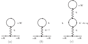
Figure 7: Hartree diagrams discussed in the text.

A similar analysis is valid for diagram (c). Its phase factors are the same as in diagram (a) and again one has two contributions. The first one, coming from the uncorrelated averaging, leads to a self-energy containing only the ${\bf q}=0$ contribution,

$$(i\hbar)^{2}\frac{N}{A^{2}} \;V^{b,b_{1}}({\bf q}=0)G_{{\bf k}}^{b_{1}}(t,t^{\prime})G_{{\bf k}}^{b_{1}}(t^{\prime},t)$$

$$\times \;V^{b_{1},b^{\prime}}({\bf q}=0)G_{m^{\prime}}^{b^{\prime}}(t^{\prime},t^{\prime}),$$ (32)

where summation and integration over the inner variables is assumed. Since this entails the restriction ${\bf k}={\bf k}^{\prime}$, the diagram contributes to the renormalization of the WL propagator of index ${\bf k}$ in diagram (b). Therefore this is already included in a self-consistent calculation. More interesting is the second term, arising from the correlated averaging,

$$(i\hbar)^{2}\frac{1}{A^{2}} \;V^{b,b_{1}}_{m,{\bf k},{\bf k}+{\bf q},m}G_{{\bf k}+{\bf q}}^{b_{1}}(t,t^{\prime})G_{{\bf k}}^{b_{1}}(t^{\prime},t)$$

$$\times \;V^{b_{1},b^{\prime}}_{{\bf k}+{\bf q},m^{\prime},m^{\prime},{\bf k}}G_{m^{\prime}}^{b^{\prime}}(t^{\prime},t^{\prime}).$$ (33)

In this case the summation over the momentum transfer ${\bf q}$ remains unrestricted. The structure is similar to the second term of diagram (a), i.e., it corresponds to the intra-QD Hartree field, but with the additional ${\bf k}$ and ${\bf k}^{\prime}={\bf k}+{\bf q}$ WL propagators forming a Lindhard loop. The loop describes the screening of the intra-QD Hartree field by the WL carriers.

The usual procedure in the GF theory is to leave the Hartree interaction unscreened and to add the Lindhard loop of diagram (c) to the ’tadpole head’ GF of the diagram (b). This avoids the double counting of such diagrams. As a result, a nondiagonal $({\bf k},{\bf k}^{\prime})$ GF appears in the self-consistent Hartree loop of diagram (b). Alternatively, one can avoid double counting by keeping only momentum-diagonal WL propagators and leave the Lindhard loop for the screening of the Coulomb line. We have chosen this second approach, which also considerably simplifies the formalism.

A fully systematic analysis of all the possible diagrams and the action of the configuration averaging over them is way beyond the scope of this paper. The approximation proposed here includes the following physically important features. The random phases associated with the QD positions give rise to a ${\bf q}=0$ singularity, which is canceled out by the global charge neutrality. On the other hand, the intra-QD fields are not influenced by the phase factors and therefore are not averaged out. The same is true for the local WL charges that respond to these fields and induce their screening.

References

- Bimberg et al. (1998) D. Bimberg, M. Grundmann, and N. N. Ledentsov, Quantum Dot Heterostructures (Wiley, New York, 1998).
- Michler (2003) P. Michler, ed., Single Quantum Dots: Fundamentals, Applications, and New Concepts, Topics in Applied Physics (Springer, Berlin, 2003).
- Nakamura (1998) A. Nakamura, Science 281, 956 (1998).
- Jain et al. (2000) S. C. Jain, M. Willander, J. Narayan, and R. V. Overstraeten, J. Appl. Phys. 87, 965 (2000).
- Damilano et al. (1999) B. Damilano, N. Grandjean, F. Semond, J. Massies, and M. Leroux, Appl. Phys. Lett. 75, 962 (1999).
- Kalliakos et al. (2004) S. Kalliakos, T. Bretagnon, P. Lefebvre, T. Taliercio, B. Gil, N. Grandjean, B. Damilano, A. Dussaigne, and J. Massies, J. Appl. Phys. 96, 180 (2004).
- Krestnikov et al. (2002) I. L. Krestnikov, N. N. Ledentsov, A. Hoffmann, D. Bimberg, A. V. Sakharov, W. V. Lundin, A. F. Tsatsul’nikov, A. S. Usikov, and Z. I. Alferov, Phys. Rev. B 66, 155310 (2002).
- Oliver et al. (2003) R. A. Oliver, G. A. D. Briggs, M. J. Kappers, C. J. Humphreys, S. Yasin, J. H. Rice, J. D. Smith, and R. A. Tayler, Appl. Phys. Lett. 83, 755 (2003).
- Vurgaftman and Meyer (2003) I. Vurgaftman and J. R. Meyer, J. Appl. Phys. 94, 3675 (2003).
- Chuang and Chang (1996) S. L. Chuang and C. S. Chang, Phys. Rev. B 54, 2491 (1996).
- Bernardini et al. (1997) F. Bernardini, V. Fiorentini, and D. Vanderbilt, Phys. Rev. Lett. 79, 3958 (1997).
- Bernardini and Fiorentini (1998) F. Bernardini and V. Fiorentini, Phys. Rev. B. 57, R9427 (1998).
- Cingolani et al. (2000) R. Cingolani, A. Botchkarev, H. Tang, H. Morko , G. Traetta, G. Coli, M. Lomascolo, A. D. Carlo, F. D. Sala, and P. Lugli, Phys. Rev. B 61, 2711 (2000).
- Ranjan et al. (2003) A. Ranjan, G. Allen, C. Priester, and C. Delerue, Phys. Rev. B 68, 115305 (2003).
- Bockelmann and Egeler (1992) U. Bockelmann and T. Egeler, Phys. Rev. B 46, 15574 (1992).
- Vurgaftman et al. (1994) I. Vurgaftman, Y. Lam, and J. Singh, Phys. Rev. B 50, 14309 (1994).
- Brasken et al. (1998) M. Brasken, M. Lindberg, M. Sopanen, H. Lipsanen, and J. Tulkki, Phys. Rev. B 58, R15993 (1998).
- Magnusdottir et al. (2003) I. Magnusdottir, S. Bischoff, A. V. Uskov, and J. Mrk, Phys. Rev. B 67, 205326 (2003).
- Nielsen et al. (2004) T. R. Nielsen, P. Gartner, and F. Jahnke, Phys. Rev. B 69, 235314 (2004).
- Schneider et al. (2004) H. C. Schneider, W. W. Chow, and S. W. Koch, Phys. Rev. B 70, 235308 (2004).
- De Rinaldis et al. (2004) S. De Rinaldis, I. D’amico, and F. Rossi, Phys Rev. B 69, 235316 (2004).
- Andreev and O’Reilly (2000) A. D. Andreev and E. P. O’Reilly, Phys. Rev. B 62, 15851 (2000).
- Bagga et al. (2003) A. Bagga, P. K. Chattopadhyay, and S. Ghosh, Phys. Rev. B 68, 155331 (2003).
- Fonoberov and Balandin (2003) V. A. Fonoberov and A. A. Balandin, J. Appl. Phys. 94, 7178 (2003).
- Sheng et al. (2005) W. Sheng, S.-J. Cheng, and P. Hawrylak, Phys. Rev. B 71, 035316 (2005).
- Williamson et al. (2000) A. J. Williamson, L. W. Wang, and A. Zunger, Phys. Rev. B 62, 12963 (2000).
- Bester and Zunger (2005) G. Bester and A. Zunger, Phys. Rev. B 71, 045318 (2005).
- Schulz and Czycholl (2005) S. Schulz and G. Czycholl, Phys. Rev. B 72, 165317 (2005).
- Wojs et al. (1996) A. Wojs, P. Hawrylak, S. Fafrad, and L. Jacak, Phys. Rev. B 54, 5604 (1996).
- Chow et al. (1999) W. W. Chow, M. Kira, and S. W. Koch, Phys. Rev. B 60, 1947 (1999).
- Chow and Koch (1999) W. W. Chow and S. W. Koch, Semiconductor - Laser Fundamentals (Springer, Berlin, 1999).
- Haug and Koch (1994) H. Haug and S. W. Koch, Quantum Theory of the Optical and Electronic Properties of Semiconductors (World Scientific Publ., Singapore, 1994), 3rd ed.
- Levinshtein et al. (2001) M. R. Levinshtein, S. L. Rumyantsev, and M. S. Shur, eds., Properties of Advanced Semiconductor Materials GaN, AlN, InN, BN, SiC, SiGe (John Wiley & Sons, Inc., New York, 2001), GaN: pp 1-30 (V. Bourgrov, et al.); InN: pp 49-66 (A. Zubrilov, et al.).
- Wu and Walukiewicz (2003) J. Wu and W. Walukiewicz, Superlattices and Microsctrutures 34, 63 (2003).
- Zang et al. (2004) H. Zang, E. J. Miller, E. T. Yu, C. Poblenz, and J. S. Speck, J. Vac. Sci. Technol. B 22, 2169 (2004).
- Lai et al. (2002) C. Y. Lai, M. Hus, W.-H. Chang, K.-U. Tseng, C.-M. Lee, C.-C. Chuo, and J.-I. Chyi, J. Appl. Phys. 91, 531 (2002).
- Lin et al. (2002) Y.-S. Lin, K.-J. Ma, C. Hsu, Y.-Y. Chung, C.-W. Liu, S.-W. Feng, Y.-C. Chang, C. C. Yang, H.-W. Chuang, C.-T. Kuo, et al., Appl. Phys. Lett. 80, 2571 (2002).
- Doniach and Sondheimer (1998) S. Doniach and E. H. Sondheimer, Green’s functions for solid state physicists (Imperial College Press, London, 1998).