Ring-shaped luminescence pattern in biased quantum wells studied as a steady state reaction front

Abstract

Under certain conditions, focused laser excitation in semiconductor quantum well structures can lead to charge separation and a circular reaction front, which is visible as a ring-shaped photoluminescence pattern. The diffusion-reaction equations governing the system are studied here with the aim of a detailed understanding of the steady state. The qualitative asymmetry in the sources for the two carriers is found to lead to unusual effects which dramatically affect the steady-state configuration. Analytic expressions are derived for carrier distributions and interface position for a number of cases. These are compared with steady-state information obtained from simulations of the diffusion-reaction equations.

I Introduction

In mid-2002, two semiconductor-optics experimental groups reported dramatic ring-shaped photoluminescence patterns when a focused laser was used to excite electron-hole pairs near a coupled quantum well system biased with an electric field ring_butov-nature ; ring_snoke-nature . Despite initial speculation invoking Bose-Einstein condensation of excitons, it was later found that the luminescence ring is well-explained by classical reaction-diffusion dynamics of the electrons and holes ring_snoke-thy ; Butov-etal_ring-thy_PRL04 . The idea is that there is net hole injection into the quantum well near the laser irradiation spot, together with an electron source due to leakage current that is roughly uniform across the two-dimensional (2D) quantum well plane. This combination can lead to a charge-separated steady state configuration, with a circular hole-rich island sustained by the localized hole source in an electron-rich sea. The interface, where outward-diffusing holes recombine with inward-diffusing electrons, is the luminescence ring.

The position of the interface, i.e., the radius of the luminescence ring, is not well-understood theoretically, despite some theoretical Butov-etal_ring-thy_PRL04 ; DenevSimonSnoke_SolidStateComm_apr05 and experimental Snoke-Pfeiffer_beyond-simple_june04 ; DenevSimonSnoke_SolidStateComm_apr05 efforts. While a full understanding may or may not require extra ingredients in addition to the diffusion-reaction model DenevSimonSnoke_SolidStateComm_apr05 , a thorough study of the behavior of the interface position within the diffusion model is certainly a necessary first step. The present Article fills this gap by presenting a detailed analysis of the steady state, addressing aspects such as the position and width of interface, density distributions, etc. There are a number of length scales in the problem which we identify cleanly. The phenomenon is put into the context of previous theoretical studies of steady-state reaction fronts and variations thereof BenNaimRedner_front_JPhys92 ; LeeCardy_PRE94 ; Krapivsky_front_PRE95 ; Cornell-Droz_PRL93 ; GalfiRacz_PRA88 ; Barkema-Cardy_reaction-front_PRE96 ; Shipilevsky_reaction_island-growth_PRE04 ; Shipilevsky_reaction_island_PRE03 ; CornellDrozChopard_PRA91 . By considering various possible relative values of the tunneling decay rates of the two carrier species, we clarify the roles of the tunneling strengths in determining the steady-state configuration. A curious feature of the steady state is that the reaction zone has, in addition to the sharp interface, an extended feature on one side where the luminescence does not vanish but instead is a nonzero constant. This aspect turns out to have a drastic influence on the interface position and the overall steady-state structure, which we explain in detail.

In comparison with previous theoretically studied diffusion-annihilation systems BenNaimRedner_front_JPhys92 ; LeeCardy_PRE94 ; Krapivsky_front_PRE95 ; Cornell-Droz_PRL93 ; GalfiRacz_PRA88 ; Barkema-Cardy_reaction-front_PRE96 ; Shipilevsky_reaction_island-growth_PRE04 ; Shipilevsky_reaction_island_PRE03 ; CornellDrozChopard_PRA91 , the present problem has several unusual features which justify an extended study. These include the single-particle (tunneling) decay of one or both species, and the fact that one of the reacting species has a spatially extended source spanning both sides of the interface. In addition, while diffusion-controlled reaction interfaces and patterns have been studied in a wide variety of chemical, biological and fluid flow contexts Hohenberg-Cross_RMP93 ; Gollub-Langer_RMP99 ; Koch-Meinhardt_RMP94 , they are rather novel in electronic systems. Indeed, this may well be the only currently known example of a diffusion-limited nonequilibrium reaction front or pattern in electronic systems. Furthermore, there is the intriguing possibility of studying quantum phenomena in the ring region LevitovSimonsButov_modln_PRL05 ; LevitovSimonsButov_modln_cm_mar05 , where the carriers have had time to cool down to quantum degeneracy.

Sec. II introduces the diffusion-reaction equations, simplifying source details, and also presents the important length scales. Sec. III contains the analysis of the steady state and the main results of this Article. In Sec. IV, we point out some limitations of the current model and put the current project into context by briefly reviewing the relevant theoretical literature. In Sec. V, our calculations on the ring radius are put into perspective by discussing experimental issues and other calculations. The method used for numerical evolution of the diffusion-reaction equations is outlined in App. A.

II Diffusion-reaction model

For experimental details beyond what is sketched here, the reader is referred to Refs. ring_butov-nature ; ring_snoke-nature ; Snoke-Pfeiffer_beyond-simple_june04 ; Butov_jphys-review_2004 . The phenomenon occurs in a two-dimensional quantum well system, either a single well or two closely separated parallel wells. Electron-hole pairs are created in the vicinity of the well(s), mainly in the substrate, by a focused laser excitation.

A voltage is applied across the well(s) using conducting electron-rich (n⁺) regions on both sides of the well(s) as leads. The original motivation was to enhance the lifetime of excitons or electron-hole gases by spatially separating electrons and holes in the direction transverse to the well(s). A band-structure cartoon of the experimental setup is shown in the inset of Fig. 1. Due to the electric field bias, there is an influx current of electrons into the well as well as a tunneling-out process. In addition, the holes can tunnel out in the other direction; this corresponds to an electron from the left lead or substrate filling up one of the hole states in the well. The three processes are shown by arrows in the Fig. 1 inset. Note that there is no source of holes due to the biasing. Holes are only created by photo-excitation.

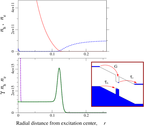
Figure 1: Top panel: steady state carrier density distributions. $n_{\rm h}$ dominates at small $r$ and $n_{\rm e}$ dominates at large $r$. Bottom panel: luminescence profile. Dashed and solid lines correspond to $P_{\rm e}\neq 0$ and $P_{\rm e}=0$ respectively. The hole excess $P_{\rm h}-P_{\rm e}$ is the same in the two cases, so that the only difference is in the structure around $r=0$. Lower-right inset: band-structure schematic (single well). Arrows indicate tunneling processes described in text.

Incorporating the above effects, one can write down two-dimensional diffusion-annihilation equations for the densities of holes ($n_{\rm h}$) and electrons ($n_{\rm e}$) within the quantum well(s):

$$\frac{\partial n_{\rm h}}{\partial{t}}~{} =~{}D_{\rm h}\nabla^{2}n_{\rm h}~{}+~{}P_{\rm h}e^{-r^{2}/l_{\rm L}^{2}}-~{}\gamma n_{\rm h}n_{\rm e}~{}-~{}\frac{1}{\tau_{\rm h}}n_{\rm h}$$ (1a)

$$\frac{\partial n_{\rm e}}{\partial{t}}~{} =~{}D_{\rm e}\nabla^{2}n_{\rm e}~{}+~{}P_{\rm e}e^{-r^{2}/l_{\rm L}^{2}}-~{}\gamma n_{\rm h}n_{\rm e}~{}+G-~{}\frac{1}{\tau_{\rm e}}n_{\rm e}$$ (1b)

The $D_{\rm h,e}$ are diffusion constants. The $n_{\rm h,e}/\tau_{\rm h,e}$ terms model decay due to carriers tunneling out of the well(s), the $\tau$’s being tunneling lifetimes. $G$ is the spatially uniform source term for electrons, which is absent for holes. The $\gamma$ terms represent electron-hole recombination. The $P_{\rm h,e}$ terms are the laser excitation terms; the carriers are focused onto a spot roughly of radius $l_{\rm L}$.

By numerically evolving Eqs. (1) in time, one can determine the steady-state carrier distributions and luminescence after $P_{\rm h,e}$ are turned on. A typical steady-state distribution, obtained with $P_{\rm h}>P_{\rm e}$, is shown in Fig. 1. The simulation (App. A) is one-dimensional, so that radial plots are sufficient. The steady state displays a species-separated configuration, together with a peak in the luminescence marking the interface, as described previously. For $P_{\rm e}\neq 0$, the luminescence profile also shows an inner peak near $r=0$, corresponding roughly to a central luminescence spot observed experimentally.

Typical values of the parameters are taken to be of the following orders, $D$’s: several cm²/s, $\tau$’s: $10^{-4}$ s, $\gamma$: $10^{-3}$ s^-1cm², $l_{\rm L}$: $10^{-3}$ cms, $G$: $10^{15}$ s^-1cm^-2, and $Pl_{\rm L}^{2}$’s: $10^{12}$ s^-1. Units will be omitted in the rest of this Article.

Eqs. (1), with several variations, was proposed in Refs. Butov-etal_ring-thy_PRL04 ; ring_snoke-thy as the luminescence ring mechanism, and studied further in Refs. Snoke-Pfeiffer_beyond-simple_june04 ; DenevSimonSnoke_SolidStateComm_apr05 ; SimonPfeiffer_dynamics_PRB05 ; LevitovSimonsButov_modln_cm_mar05 ; LevitovSimonsButov_modln_PRL05 . For a restricted case, Ref. Butov-etal_ring-thy_PRL04 also contains a minimal analytic treatment of the steady state.

For the charge separation phenomenon, we need more holes diffusing out of the excitation region than electrons. In previous studies ring_snoke-thy ; Butov-etal_ring-thy_PRL04 ; Snoke-Pfeiffer_beyond-simple_june04 ; DenevSimonSnoke_SolidStateComm_apr05 , the philosophy has been to invoke differences of unknown origin in the efficiency of accumulation in the well(s), i.e., to use $P_{\rm h}>P_{\rm e}$ without detailed explanation. The current understanding of carrier asymmetry is thus unsatisfactory. In fact, it is possible to have an excess of holes and a resulting luminescence ring with $P_{\rm h}=P_{\rm e}$. However, the present author will postpone to a future publication an analysis of the source asymmetry and of the inner spot structure.

Since we neglect the inner structure in this study, it is convenient to drop the electron source altogether ($P_{\rm e}=0$), and assume a point source for the holes, i.e., $P_{\rm h}e^{-r^{2}/l_{\rm L}^{2}}$ is replaced by $P_{\rm x}\delta({\bf r})$. For comparison with the numeric simulations, where a finite $l_{\rm L}$ has been used, the correspondence is $P_{\rm x}\equiv\pi l_{\rm L}^{2}P_{\rm h}$. This is obtained by equating outward flux for the point and gaussian sources. One result of omitting the electron source is the absence of an inner luminescence spot (Fig. 1, solid line in lower panel). Moreover, the expressions for hole density in Sec. III will diverge at the illumination spot. This (minor) un-physical result is a result of the un-physical “point” source.

We now identify the length scales present in the problem. The two most important ones are the depletion lengths for electrons and holes, $l_{\rm e}=\sqrt{D_{\rm e}\tau_{\rm e}}$ and $l_{\rm h}=\sqrt{D_{\rm h}\tau_{\rm h}}$. The depletion lengths provide the length scales for the variation of steady state densities, analogous to the diffusion lengths $\sqrt{Dt}$ in the literature on time-dependent front formation between two initially separated reactants Krapivsky_front_PRE95 ; GalfiRacz_PRA88 ; CornellDrozChopard_PRA91 ; LeeCardy_PRE94 , where $\sqrt{Dt}$ gives the spatial variation length scale after time $t$.

The ratio of the source strengths, $P_{\rm x}$ and $G$, provides a third length scale, which we define as $l_{\rm src}=\sqrt{P_{\rm x}/{\pi}G}\,$. The radius of the ring-shaped interface increases monotonically with the length $l_{\rm src}$. The interface radius $l_{\rm R}$ itself, and the interface width $l_{\rm w}$, are not input parameters in the problem but emerge from the analysis as important length scales. We are interested in cases where the interface is sharp, i.e., $l_{\rm w}\ll l_{\rm R}$.

Other lengths appearing in the problem can be expressed in terms of the ones introduced above.

III Analysis of steady state

Analytic treatment of the steady state is simpler if one neglects the hole tunneling ($\tau_{\rm h}\rightarrow\infty$), so that the hole depletion length $l_{\rm h}=\sqrt{D_{\rm h}\tau_{\rm h}}$ disappears from the problem. Note that a finite $\tau_{\rm e}$ is necessary to provide the uniform electron background at large $r$. It is also convenient to first consider an infinitely sharp interface ($l_{\rm w}=0$). In addition, the treatment in Ref. Butov-etal_ring-thy_PRL04 neglects the electron density on the hole side of the interface, and vice versa. We will consider this simplified model in III.1, first without assuming anything about $l_{\rm R}/l_{\rm e}$, and then writing out both $l_{\rm R}\ll l_{\rm e}$ and $l_{\rm R}\gg l_{\rm e}$ limits.

In III.2, corrections due to nonzero $n_{\rm e}$ in the hole side are derived. In III.3, a finite $\tau_{\rm h}$ is re-inserted, and in III.4 the width of the sharp interface itself is studied.

III.1 Simplified model

With $\tau_{\rm h}\rightarrow\infty$, the equations for steady state are

$$D_{\rm h}\nabla^{2}n_{\rm h}~{}+~{}P_{\rm x}\delta({\bf r})-~{}\gamma n_{\rm h}n_{\rm e}~{} =~{}0$$ (2a)

$$D_{\rm e}\nabla^{2}n_{\rm e}~{}-~{}\gamma n_{\rm h}n_{\rm e}~{}+G-~{}\frac{1}{\tau_{\rm e}}n_{\rm e}~{} =~{}0$$ (2b)

If the hole and electron densities are strictly zero outside and inside the ring respectively, then the nonlinear reaction terms in Eqs. (2) then drop out both inside and outside the ring. The resulting linear equations can be exactly solved:

$$n_{\rm h}({\bf r})~{} =~{}\frac{P_{\rm x}}{2\pi D_{\rm h}}\,\ln\left(\frac{l_{\rm R}}{r}\right)\,\,\theta(l_{\rm R}-r)\,\,,$$ (3)

$$n_{\rm e}({\bf r})~{} =~{}G\tau_{\rm e}\left[1~{}-~{}\frac{K_{0}\left({r/l_{\rm e}}\right)}{K_{0}\left({l_{\rm R}/l_{\rm e}}\right)}\,\right]\,\theta(r-l_{\rm R})\,\,.$$ (4)

Here $K_{\nu}(x)$ is a modified Bessel function of the second kind.

Note that Eq. (3) is very similar to Eq. (17) of Ref. BenNaimRedner_front_JPhys92 , where also a steady state is analyzed. On the other hand, Eq. (4) involves a length scale ($l_{\rm e}$), which is not so common in previous studies of steady state fronts. Instead, it resembles more the time-dependent case of Refs. GalfiRacz_PRA88 ; CornellDrozChopard_PRA91 ; LeeCardy_PRE94 ; Krapivsky_front_PRE95 , where the corresponding length scale is determined by the time $t$, analogously to our $\tau_{\rm e}$.

In the $l_{\rm R}\ll l_{\rm e}$ limit, Eq. (4) can be written approximately as

$$n_{\rm e}({\bf r})~{}=~{}G\tau_{\rm e}\left[1~{}-~{}\frac{\ln\left({r/l_{\rm e}}\right)}{\ln\left({l_{\rm R}/l_{\rm e}}\right)}\,\theta(l_{\rm e}-r)\right]\,\theta(r-l_{\rm R})\,\,,$$ (5)

provided we are not interested in the $n_{\rm e}(r)$ behavior for $r\gtrsim l_{\rm e}$. In the limit $l_{\rm R}\gg l_{\rm e}$:

$$n_{\rm e}({\bf r})~{}=~{}G\tau_{\rm e}\left[1~{}-~{}\frac{e^{-r/l_{\rm e}}/\sqrt{r}}{e^{-l_{\rm R}/l_{\rm e}}/\sqrt{l_{\rm R}}}\,\right]\,\theta(r-l_{\rm R})\,\,.$$ (6)

With the expressions for the densities, one can now match the electron influx and hole outflux currents ($j=-D\nabla{n}$) to determine the ring radius $l_{\rm R}$ in the simplified model:

$$D_{\rm h}\left[\frac{P_{\rm x}}{2\pi D_{\rm h}}\frac{1}{l_{\rm R}}\right]~{}=~{}D_{\rm e}\left[\frac{G\tau_{\rm e}}{l_{\rm e}}\frac{K_{1}\left({l_{\rm R}/l_{\rm e}}\right)}{K_{0}\left({l_{\rm R}/l_{\rm e}}\right)}\right]\;\;.$$ (7)

This equation can be solved numerically to give the ring position $l_{\rm R}$ as a function of the hole source strength $P_{\rm x}$, or more “universally”, to express $l_{\rm R}/l_{\rm e}$ as a function of $(l_{\rm src}/l_{\rm e})^{2}$.

The hole diffusion constant $D_{\rm h}$ drops out, and so the interface position is independent of $D_{\rm h}$. In addition, the recombination rate $\gamma$ does not enter because of the zero-width approximation for the interface. This approximation turns out to be surprisingly good as far as $l_{\rm R}$ is concerned; as long as there is a well-defined peak in the luminescence, changing $\gamma$ affects the width and height of the peak profile but not the position (Fig. 2a). We also note that the two source parameters enter only as the ratio $P_{\rm x}/G$ and not individually.

In the $l_{\rm R}\ll l_{\rm e}$ and $l_{\rm R}\gg l_{\rm e}$ limits, Eq. (7) can be solved analytically for $l_{\rm R}$, giving respectively

$$l_{\rm R}=l_{\rm e}\exp\left[-2{\pi}Gl_{\rm e}^{2}/P_{\rm x}\right]=l_{\rm e}\exp\left[\frac{-2}{(l_{\rm src}/l_{\rm e})^{2}}\right]\;\;$$ (8)

and

$$l_{\rm R}=P_{\rm x}/2{\pi}Gl_{\rm e}=l_{\rm src}^{2}/2l_{\rm e}$$ (9)

Eqs. (3), (5) and (8) have been obtained previously Butov-etal_ring-thy_PRL04 . Ref. Butov-etal_ring-thy_PRL04 has a spurious $D_{\rm h}^{-1}$ factor in the exponent of expression (8) for $l_{\rm R}$.

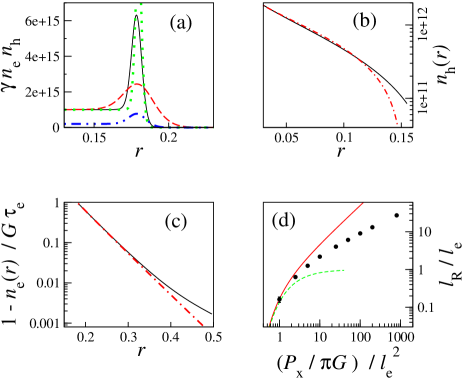
Figure 2: Assessment of the simple model in Sec. III.1 and in Ref. Butov-etal_ring-thy_PRL04 . (a) Luminescence profiles ($\gamma n_{\rm h}n_{\rm e}$) shown for situations in which $l_{\rm src}$, $l_{\rm e}$ are fixed but other parameters vary. Compared to the solid curve, dashed curve has $\gamma$ decreased by factor 25, while dotted curve has $D_{\rm h}$ decreased by a factor 5, all other parameters remaining fixed. Dash-dot curve has $G$ and $P_{\rm x}$ decreased by factor 5, while keeping the ratio $P_{\rm x}/G$ fixed. (b) Solid line is hole density $n_{\rm h}(r<l_{\rm R})$ in hole-rich side of interface, from simulation. Dash-dot line shows best fit of the form $\sim\ln(l_{\rm R}/r)$. (c) Electron density distribution, $n_{\rm e}(r>l_{\rm R})$, from simulation, normalized to and subtracted from $n_{\rm e}(\infty)=G\tau_{\rm e}$. Dash-dot line is fit to $K_{0}(r/l_{\rm e})$, Eq. (4). (d) Radius of ring, in units of the electron depletion length $l_{\rm e}$, plotted as a function of hole source strength $P_{\rm x}$, in units of $\pi{G}l_{\rm e}^{2}$.

The theory developed in this section, based on the approach of Ref. Butov-etal_ring-thy_PRL04 , is now evaluated by comparing with data from numeric simulation (App. A) of the diffusion-reaction equations. In Fig. 2a, luminescence profiles have been plotted for several cases to show that the ring radius remains unchanged if the recombination rate $\gamma$ is changed (an assumption of the theory), if the hole diffusion constant $D_{\rm h}$ is changed (a prediction of the $\tau_{\rm h}\rightarrow\infty$ theory), and if the electron injection current density $G$ and hole injection rate $P_{\rm x}$ are both changed while their ratio $P_{\rm x}/G=\pi l_{\rm src}^{2}$ is kept fixed (another prediction of the theory). In each of these cases the width of the interface is modified, as discussed in Sec. III.4.

In Fig. 2b, the steady state hole density profile obtained from simulation of Eqs. (1) is compared with the logarithmic prediction, Eq. (3). The agreement is reasonable but imperfect; an improvement will be found in the next section.

In Fig. 2c, the expression (4) for the electron densities outside the ring, $n_{\rm e}(r>l_{\rm L})$, is tested against simulation data. There is some deviation at large distances, which remains unexplained. The density profiles of Figs. 2b and 2c are taken from a steady state solution with $l_{\rm R}\approx 0.18$.

Finally, in Fig. 2d, the radius of the circular interface, obtained from direct simulation of Eq. (1), is plotted against hole injection intensities $P_{\rm x}$. This is compared with Eq. (7), plotted as a solid line. The $l_{\rm R}\ll l_{\rm e}$ limit is shown by a dashed line. For larger radii ($l_{\rm R}>l_{\rm e}$ and $l_{\rm src}>l_{\rm e}$), the prediction for the radius is seriously at odds with the numerical results. The simulations suggest that the dependence on $P_{\rm x}/G$ follows a lower exponent than the linear dependence obtained in this section. This discrepancy is corrected in the next section.

III.2 Corrections from “dark” interior

We now turn our attention to the hole-rich region within the ring, at radial distances $r<l_{\rm R}$, far enough from the reaction front so that $n_{\rm h}\gg n_{\rm e}$. We will now encounter effects of the extended source term for the electrons, i.e., of the position-independent $G$. Taking account of these effects turns out to be the key to overcoming the failure in Sec. III.1 to predict the ring radius for $l_{\rm R}\gg l_{\rm e}$.

Some of the figures published by Ref. ring_butov-nature ; Butov-etal_ring-thy_PRL04 suggest a nonzero luminescence intensity in the nominally dark region between inner spot and ring. The small but nonzero intensity in the ring interior seems to be roughly constant between the inner spot and the ring, but a more quantitative statement is hard to extract from the published figures. To the best of the present author’s knowledge, this feature has not been explained previously.

In numerical results (e.g., in Fig. 1 and also in Fig. 1c of Ref. Butov-etal_ring-thy_PRL04 ), one feature of the luminescence ($\gamma n_{\rm h}n_{\rm e}$) curve is that it is nonzero and very nearly constant in most of the supposedly dark interior of the ring. The constant value is found to be equal $G$, the electron influx density. In other words, our reaction zone has an “extended” part in the hole side of the interface.

To explain the constant luminescence for $r<l_{\rm R}$, as seen in the numeric simulations and possibly in the experiments, we relax the assumption that $n_{\rm e}(r)$ vanishes completely inside the ring ($r<l_{\rm R}$). In the steady-state equation for the electron density, Eq. (2b), the tunneling term can be neglected compared to $G$ because $n_{\rm e}(r<l_{\rm R})\ll n_{\rm e}(\infty)=G\tau_{\rm e}$. The diffusion term is also small because, away from the interface, $n_{\rm e}$ is small and smoothly varying. (This is justified more rigorously, a posteriori, in App. B.) We are left with $\gamma n_{\rm h}(r)n_{\rm e}(r)\approx G$, as required.

A finite $\gamma n_{\rm h}n_{\rm e}$ also affects the steady-state hole density distribution. Feeding $\gamma n_{\rm h}n_{\rm e}=G$ into Eq. (2a), we get a correction to the expression (3) for the hole density:

$$n_{\rm h}(r<l_{\rm R})~{}=~{}\frac{P_{\rm x}}{2\pi D_{\rm h}}\,\ln\left(\frac{l_{\rm R}^{\prime}}{r}\right)~{}+~{}\frac{G}{4D_{\rm h}}r^{2}\\ =~{}\frac{P_{\rm x}}{2\pi D_{\rm h}}\,\left[\ln(l_{\rm R}^{\prime}/r)~{}+~{}\frac{r^{2}}{2l_{\rm src}^{2}}\right]\,\,,$$ (10)

with $l_{\rm R}^{\prime}\neq l_{\rm R}$. Assuming the luminescence peak to be sharp enough, using the condition $n_{\rm h}(r=l_{\rm R})=0$ yields $l_{\rm R}^{\prime}=l_{\rm R}\exp[-l_{\rm R}^{2}/2l_{\rm src}^{2}]$.

The lower inset to Fig. 3 shows that Eq. (10), with the $(G/4D_{\rm h})r^{2}$ term included, provides perfect agreement with the numerical simulations. This can be compared to the previous attempt (Fig. 2b). The same inset also shows the electron density in the hole region (much magnified), perfectly obeying

$$n_{\rm e}(r<l_{\rm R})=\frac{G/\gamma}{n_{\rm h}(r<l_{\rm R})}=\frac{2D_{\rm h}/\gamma}{l_{\rm src}^{2}\ln(l_{\rm R}^{\prime}/r)+{\tfrac{1}{2}}r^{2}}\;\;.$$ (11)

Note that the decay of $n_{\rm e}$ as one moves away from the interface is not exponential or even power-law, but much weaker.

The $l_{\rm R}^{\prime}$ that gives the best fit to the $n_{\rm h}$ and $n_{\rm e}$ curves is also in excellent agreement with the prediction above.

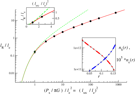
Figure 3: Radius, in units of $l_{\rm e}$, plotted against $P_{\rm x}$, in units of ${\pi}Gl_{\rm e}^{2}$. The dots are from numerical simulations, the solid line is the improved theory of Sec. III.2, and the dashed line is the theory of Sec. III.1. The upper inset displays same curves in linear scale to give a sense of how the curves cross over from inverse-exponential to power-law behavior as $l_{\rm src}$ crosses $l_{\rm e}$. In the lower inset: Negative-slope curve is $n_{\rm h}(r<l_{\rm R})$, fitted (thick dashed line) with Eq. (10). Positive-slope curve is $n_{\rm e}(r<l_{\rm R})$, magnified by five orders of magnitude, with thick dashed line showing fit by Eq. (11).

An even more dramatic improvement occurs with the prediction for the radius, which we determine, as before, by imposing $D_{\rm h}|n_{\rm h}^{\prime}(l_{\rm R})|=D_{\rm e}|n_{\rm e}^{\prime}(l_{\rm R})|$:

$$\frac{1}{2l_{\rm R}}\left(l_{\rm src}^{2}-l_{\rm R}^{2}\right)~{}=~{}l_{\rm e}\;\frac{K_{1}(l_{\rm R}/l_{\rm e})}{K_{0}(l_{\rm R}/l_{\rm e})}\;\;.$$ (12)

Fig. 3 shows how the peak postions obtained from direct simulation of the diffusion-reaction Eqs. (1) are perfectly explained by Eq. (12). The discrepancy of our original attempt following Ref. Butov-etal_ring-thy_PRL04 , as shown in Fig. 2(a), has been solved.

The $l_{\rm R}\gg l_{\rm e}$ and $l_{\rm R}\ll l_{\rm e}$ limits are respectively

$$l_{\rm R}=~{}-l_{\rm e}+\sqrt{l_{\rm e}^{2}+(P_{\rm x}/\pi{G})}~{}=~{}-l_{\rm e}+\sqrt{l_{\rm e}^{2}+l_{\rm src}^{2}}$$

and

$$l_{\rm R}=l_{\rm e}\exp\left[-\frac{2l_{\rm e}^{2}}{l_{\rm src}^{2}-l_{\rm R}^{2}}\right]\approx l_{\rm e}\exp\left[-\frac{2l_{\rm e}^{2}}{l_{\rm src}^{2}}\right]\;\;.$$

From the solution of Eq. (12), e.g., from Fig. 3, one observes that $l_{\rm src}/l_{\rm e}$ also tends to be large for $l_{\rm R}\gg l_{\rm e}$. Using this additional information, the $l_{\rm R}\gg l_{\rm e}$ expression reduces to $l_{\rm R}\approx l_{\rm src}=\sqrt{P_{\rm x}/{\pi}G}$. This explains the straight line in the log-log plot of Fig. 3 for large $l_{\rm R}/l_{\rm e}$. The line has slope half of that in the case of the simple theory without interior correction, Fig. 2(a), where the behavior is $l_{\rm R}\propto{P}_{\rm x}$.

It is remarkable that the tiny $n_{\rm e}(r<l_{\rm R})$, orders of magnitude smaller than $G\tau_{\rm e}$ or $n_{\rm h}(r<l_{\rm R})$, actually modifies the global structure of the steady-state configuration.

III.3 Finite hole tunneling

We now relax the approximation of infinite hole leakage timescale $\tau_{\rm h}$, so that the hole depletion length $l_{\rm h}=\sqrt{D_{\rm h}\tau_{\rm h}}$ is finite and can play a role. Eq. (3) for the hole density is now corrected to

$$n_{\rm h}(r)~{}=~{}\frac{P_{\rm x}}{2\pi D_{\rm h}}\,K_{0}\left(\frac{r}{l_{\rm h}}\right)\,\,\theta(l_{\rm R}-r)\;\;.$$ (13)

For $r\ll l_{\rm h}$, the $K_{0}$ solution reduces to a logarithm, as before.

Note that, since the $K_{0}$ function does not vanish for finite arguments, the radius $l_{\rm R}$ cannot be built into $n_{\rm h}(r<l_{\rm R})$ as a boundary condition. The discontinuity in Eq. (13) suggests that the structure of the interface plays a more important role here compared to the $l_{\rm h}\rightarrow\infty$ case. In addition, Eq. (13) also allows us to infer the ring radius $l_{\rm R}$ using “physical” arguments. The discontinuity can be minimized by having $l_{\rm R}>l_{\rm h}$, because the $K_{0}(x)$ function crosses over to $\sim{e}^{-x}/\sqrt{x}$ for $x>1$. On the other hand, $l_{\rm R}$ cannot be too much larger than $l_{\rm h}$, since the hole flux also decreases exponentially for $l_{\rm R}>l_{\rm h}$. The radius is therefore expected to be slightly larger than the hole depletion length $l_{\rm h}$, for a range of parameters.

As in Sec. III.2, one should correct for nonzero $\gamma n_{\rm h}(r)n_{\rm e}(r)$, at $r<l_{\rm R}$:

$$n_{\rm h}(r<l_{\rm R})~{}=~{}\frac{P_{\rm x}}{2\pi D_{\rm h}}\,K_{0}\left(\frac{r}{l_{\rm h}}\right)~{}-~{}G\tau_{\rm h}\;\;,$$ (14)

and

$$n_{\rm e}(r<l_{\rm R})~{}=~{}\frac{2D_{\rm h}/\gamma}{l_{\rm src}^{2}K_{0}(r/l_{\rm h})-2l_{\rm h}^{2}}\;\;.$$ (15)

Since the correction to $n_{\rm h}(r)$ is a constant, the extended part of the reaction zone loses the crucial role it had for $l_{\rm h}\rightarrow\infty$ in the determination of the interface position $l_{\rm R}$. Assuming again an infinitely sharp interface at $l_{\rm R}$ and equating currents,

$$\frac{P_{\rm x}}{2\pi l_{\rm h}}\,K_{1}(l_{\rm R}/l_{\rm h})~{}=~{}Gl_{\rm e}\,\frac{K_{1}(l_{\rm R}/l_{\rm e})}{K_{0}(l_{\rm R}/l_{\rm e})}\;\;.$$ (16)

In the $l_{\rm R}\gg l_{\rm e}$, $l_{\rm R}\gg l_{\rm h}$ limit,

$$l_{\rm R}=\tfrac{1}{2}l_{\rm h}\;W_{0}\left(\frac{P_{\rm x}/4G}{l_{\rm e}^{2}l_{\rm h}^{2}}\right)=\tfrac{1}{2}l_{\rm h}\;W_{0}\left(\frac{\pi}{4}\left[l_{\rm src}/\sqrt{l_{\rm e}l_{\rm h}}\right]^{4}\right)\;.$$ (17)

Here $W_{0}(x)$ is the principal branch of the Lambert $W$ function LambertW . The large-$l_{\rm R}$ behavior for comparable $l_{\rm h}$ and $l_{\rm e}$ is thus logarithm-like rather than power-law.

Unsurprisingly, in the $l_{\rm R}\ll l_{\rm e}$, $l_{\rm R}\ll l_{\rm h}$ limit, one recovers the $l_{\rm R}\ll l_{\rm e}$ limit of Secs. III.1 and III.2 , $l_{\rm R}=l_{\rm e}\exp[-2l_{\rm e}^{2}/l_{\rm src}^{2}]$.

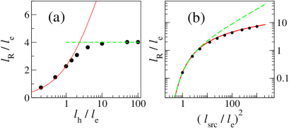
Figure 4: Ring radius with finite hole tunneling. (a) Variation with hole depletion length $l_{\rm h}$, for $P_{\rm x}=25{\pi}G$. (b) Variation with $P_{\rm x}/{\pi}G$, for $l_{\rm h}=\sqrt{2}l_{\rm e}$. In each plot, dots are from direct simulation of Eqs. (1). Solid curves are the prediction of Eq. (16) and dashed curves are the $l_{\rm h}=\infty$ result, Eq. (12).

Fig. 4a shows the dependence of the radius on the hole tunneling. At small $l_{\rm h}$, the radius obeys Eq. (16) well. As predicted, here the radius tends to be somewhat larger than but of the order of the hole depletion length $l_{\rm h}$. At large $l_{\rm h}$, the ring radius approaches the $l_{\rm h}=\infty$ result of Eq. (12). There is an intermediate range of $l_{\rm h}$ where neither equations work. For the case shown in Fig. 4a, this crossover region is $2l_{\rm e}\lesssim l_{\rm h}\lesssim 10l_{\rm e}$. Presumably, an analytic understanding of this parameter region requires taking into account the interface structure details. The author has not been able to incorporate effects of interface structure into the prediction for the radius.

Fig. 4b shows for $l_{\rm h}=\sqrt{2}l_{\rm e}$ the radius as a function of hole source intensity. For this $l_{\rm h}/l_{\rm e}$, Eq. (16) still works extremely well.

III.4 Width and structure of interface

The width $l_{\rm w}$ of steady-state reaction fronts in diffusion-limited reaction processes is known from heuristic arguments BenNaimRedner_front_JPhys92 ; Cornell-Droz_PRL93 to scale as $(D_{\rm h}D_{\rm e}/\gamma{J})^{1/3}$, where $J$ is the flux of particles entering the interface region.

In Fig. 5 the steady state interface width, obtained by simulation of Eqs. (1), is displayed as a function of various parameters. While the variations with the hole diffusion $D_{\rm h}$ and the annihilation rate $\gamma$ do follow $\pm\tfrac{1}{3}$ exponents quite closely, the dependence on the electron diffusion $D_{\rm e}$ is much weaker. To understand this, one has to consider the particle flux $J$. For both cases of infinite and finite $\tau_{\rm h}$, the flux of electrons into the interface region is $J=Gl_{\rm e}[K_{1}(l_{\rm R}/l_{\rm e})/K_{0}(l_{\rm R}/l_{\rm e})]$. There is complicated dependence on the ring position $l_{\rm R}$, but in the $l_{\rm R}\gg l_{\rm e}$ limit one can use $[K_{1}(x)/K_{0}(x)]\xrightarrow{x\gg 1}1$ to simplify:

$$l_{\rm w}\sim\left(\frac{D_{\rm h}D_{\rm e}}{\gamma{G}l_{\rm e}}\right)^{1/3}=\frac{D_{\rm h}^{1/3}D_{\rm e}^{1/6}}{\gamma^{1/3}G^{1/3}\tau_{\rm e}^{1/6}}\;\;.$$ (18)

The variation of the numerically determined width with $G$ (Fig. 5c) is also in accord with this prediction. In Figs. 5a-c the ring position $l_{\rm R}$ is unchanged.

The variation with $D_{\rm e}$ shown in Fig. 5d is more complex; in this case $l_{\rm R}$ also changes with $D_{\rm e}$. While the exponent $1/6$ works reasonably for an intermediate range of $D_{\rm e}$, there is significant deviation at larger $D_{\rm e}$ because the ring radius $l_{\rm R}$ gets smaller, leading to a breakdown of the $K_{1}/K_{0}\approx 1$ approximation. At small $D_{\rm e}$, the interface width is difficult to define because the interface becomes highly asymmetric for $D_{\rm e}\ll D_{\rm h}$, as indicated by the large error bars in Fig. 5d. In Fig. 5e both diffusion constants are varied together. The interface width is now better defined over a wide range and the exponent 1/2 (from $D_{\rm h}^{1/3}D_{\rm e}^{1/6}=D^{1/3+1/6}=D^{1/2}$) works very well.

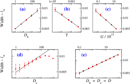
Figure 5: Width (full width at half-maximum) of luminescence peak, from steady states obtained by simulation, plotted (log-log) against various parameters. The error bars reflect the fact that one could choose half-maximum using either $G$ or zero as the base value of the luminescence $\gamma n_{\rm e}n_{\rm h}$, since $\gamma n_{\rm e}n_{\rm h}$ falls to $G$ on one side of the peak and to zero on the other side. In (c), $G$ is varied while keeping the ratio $P_{\rm x}/G=\pi l_{\rm src}^{2}$ constant. In (e), $D_{\rm h}$ and $D_{\rm e}$ are varied together. The straight lines are power-law fits with exponents (a) $1/3$, for $D_{\rm h}$, (b) $-1/3$, for $\gamma$, (c) $-1/3$, for $G$, (d) $1/6$, for $D_{\rm e}$, and (d) $1/2$, for $D=D_{\rm h}=D_{\rm e}$.

The detailed structures of $n_{\rm h,e}$ at the interface are difficult to put in closed form. Within this region $n_{\rm e}(r)$ crosses over from its $r<l_{\rm R}$ behavior, Eq. (11) or (15), to its $r>l_{\rm R}$ solution, Eq. (2b). In the same region, the hole density crosses over from its interior solution, Eq. (10) or (14), to its $r>l_{\rm R}$ solution which we have not considered yet. For $r>l_{\rm R}+l_{\rm e}$, where $n_{\rm e}$ has reached $n_{\rm e}(r=\infty)=G\tau_{\rm e}$, the hole density decays fast, as $K_{0}(r/l_{\rm out})$, with the small decay length $l_{\rm out}=\sqrt{D_{\rm h}/G\tau_{\rm e}\gamma}=l_{\rm w}\sqrt{l_{\rm w}/l_{\rm e}}$.

We will not attempt to extract details of the crossover, which can in principle be obtained with a $l_{\rm w}/l_{\rm R}$ expansion, similar to boundary-layer theory fetter-and-boundary-layer developed in the context of fluid flows near boundaries.

IV Theoretical context and limitations

Although motivated by particular solid-state experiments, it is instructive to consider this analysis in the context of theoretical investigations of steady-state diffusion-limited reaction fronts and closely-related situations. A thorough study of a simple steady state front, with diffusion and annihilation terms and equal and opposite currents, appears in Ref. BenNaimRedner_front_JPhys92 . Our calculations are in the same spirit, but we have specific source and decay terms in addition, which play crucial roles. A related (and more often studied) phenomenon is that of time-dependent fronts, where two species are initially well-segregated GalfiRacz_PRA88 ; CornellDrozChopard_PRA91 ; LeeCardy_PRE94 . Many of the same considerations apply, with powers of inverse time ($t^{-\alpha}$) playing a similar role as the particle flux $J$ does in the steady-state case. Geometries similar to ours have been considered in Refs. Shipilevsky_reaction_island_PRE03 ; Shipilevsky_reaction_island-growth_PRE04 ; island-in-sea , where one species of the reaction-annihilation pair forms an island in a sea of the other.

We have limited ourselves to the mean-field diffusion-reaction equations (1). In principle, mean-field treatments are valid only above the critical dimension, which happens to be two. At and below the critical dimension, fluctuations become important CornellDrozChopard_PRA91 ; Cornell-Droz_PRL93 ; LeeCardy_PRE94 ; Barkema-Cardy_reaction-front_PRE96 ; Krapivsky_front_PRE95 . In the 2D system of the present Article, effects of fluctuations may show up in several ways. First, the form of the annihilation term we have used, $\gamma n_{\rm h}n_{\rm e}$, can be expected to have logarithmic corrections in 2D Krapivsky_front_PRE95 . Logarithmic corrections are also expected for the power-law scaling of the width Krapivsky_front_PRE95 ; CornellDrozChopard_PRA91 ; Cornell-Droz_PRL93 . We justify the mean-field approximation by noting that almost all the quantities we have considered involve large numbers of particles so that fluctuations are unimportant.

We have assumed that the charged carriers annihilate directly, neglecting the diffusion, dissociation and quantum dynamics of bound exictons LevitovSimonsButov_modln_PRL05 ; LevitovSimonsButov_modln_cm_mar05 . Exciton diffusion might cause the observed luminescence width to be larger than what corresponds to $\gamma n_{\rm h}n_{\rm e}$ in our model, but the overall trends of Sec. III.4 are not expected to be affected severely. We have also ignored possible effects of quantum degeneracy of the charged carriers, which could change the form of the diffusion terms, so that $D_{\rm h,e}$ are themselves density-dependent DenevSimonSnoke_SolidStateComm_apr05 . All effects of coulomb interactions, including screening effects from the conducting leads Snoke-Pfeiffer_beyond-simple_june04 ; DenevSimonSnoke_SolidStateComm_apr05 ; LevitovSimonsButov_modln_cm_mar05 , have also been left out of our formulation.

V Discussion

In their brief analytic treatment of the steady state, Butov et. al. Butov-etal_ring-thy_PRL04 have assumed $l_{\rm h}=\infty$ (lack of hole tunneling decay) and $l_{\rm R}\ll l_{\rm e}$. Our results of Sec. III.3 allow an assessment of the $l_{\rm h}=\infty$ approximation (Secs. III.1, III.2 and Ref. Butov-etal_ring-thy_PRL04 ). Fig. 4a shows that it is reasonable for $l_{\rm h}\gtrsim 10l_{\rm e}$, but breaks down for smaller $l_{\rm h}$. Since $\tau_{\rm h}>\tau_{\rm e}$ is typical in the experimental realizations, the $l_{\rm h}=\infty$ results may well be experimentally relevant in some cases.

On the other hand, the $l_{\rm R}\ll l_{\rm e}$ approximation is more questionable. First, with the $l_{\rm R}\sim\exp[-\lambda/P_{\rm x}]$ behavior, a relatively small change in $P_{\rm x}$ can induce an orders-of-magnitude change in $l_{\rm R}$. This implies that fluctuations in the effective $P_{\rm x}$ would cause the ring position to fluctuate wildly, so that the stable luminescence ring pattern would be unlikely to have been observed. (Such fluctuations have also been observed in the numerical simulations for $l_{\rm R}\lesssim l_{\rm e}$.) Second, experimental data on the ring radius as a function of intensity Snoke-Pfeiffer_beyond-simple_june04 ; DenevSimonSnoke_SolidStateComm_apr05 show power-law behavior rather than any strong $\exp[-\lambda/P_{\rm x}]$-like behavior. While the relationship between $P_{\rm x}$ and the intensity is not known, it is unlikely to compensate for the $\exp[-\lambda/P_{\rm x}]$ behavior and give power-law-like $l_{\rm R}$-vs-intensity curves. It is therefore important to consider the $l_{\rm R}\gg l_{\rm e}$ case in detail, as we have done.

We now comment on the experimental $l_{\rm R}$ vs. intensity data Snoke-Pfeiffer_beyond-simple_june04 ; DenevSimonSnoke_SolidStateComm_apr05 . The non-monotonic behavior in Fig. 5 of Ref. Snoke-Pfeiffer_beyond-simple_june04 strongly indicates that the dependence of the $P_{\rm x}$ parameter of our model on the laser intensity is complicated. Note that $P_{\rm x}$ is an effective parameter measuring the amount of excess holes diffusing out of the laser irradiation region. To the best of the author’s knowledge, the process of generating excess holes has not been modeled carefully, and nothing is known conclusively about the $P_{\rm x}$-intensity dependence.

In Ref. DenevSimonSnoke_SolidStateComm_apr05 , Denev et. al. have suggested that the linear behavior of $l_{\rm R}$ vs. intensity might be due to the importance of coulomb terms which are not included in the present diffusion-reaction model. However, if the effective $P_{\rm x}$ parameter is a quadratic power of the intensity, our $l_{\rm R}\propto\sqrt{P_{\rm x}}$ prediction for $l_{\rm h}\gg l_{\rm e}$ would also show up as a linear $l_{\rm R}$-intensity result.

Our analytic results gives insight into other simulations, for example the numerical results in Fig. 1b of Ref. DenevSimonSnoke_SolidStateComm_apr05 . The fact that this curve behaves roughly logarithmically at large $l_{\rm R}$ (large $P_{\rm x}$), rather than as a power law with exponent 1/2, shows that the simulations were done using finite $\tau_{\rm h}$, with $l_{\rm h}$ not too large compared to $l_{\rm e}$. Note that the Lambert $W$ function of Eq. (17) is roughly logarithmic for large arguments, $W_{0}(x\rightarrow\infty)\approx\log{x}-\log(\log{x})$.

To summarize, motivated by semiconductor luminescence experiments, we have investigated a two-species inhomogeneous steady state arising from mean-field diffusion-annihilation equations with a localized source for one and an extended source for the other. If the holes are not allowed to have single-particle (tunneling) decay, our analysis predicts the density profiles and the radius of the ring-shaped interface with spectacular success. When both species are allowed to tunnel out, the quality of the analytic predictions is more modest. We have detailed the crossover between finite hole tunneling and zero hole tunneling behaviors of the interface position. The thorough study of the steady state within the diffusion-reaction model should serve as a baseline for evaluating the need to invoke additional physical effects for explaining experimental observations.

Appendix A Numerical simulations

The numeric steady states have been obtained by following in time the evolution of Eqs. (1). The one-dimensional spatial grid was not linear but chosen to be concentrated at smaller radial distances. The time evolution due to the diffusion terms was performed by a symmetric combination of forward and backward Euler evolution. This is sometimes called the “improved Euler method” and has error $\mathcal{O}(\delta{t}^{3})$ per time-step. The time steps $\delta{t}$ themselves were determined adaptively, and kept small enough such that the diffusion terms would not decrease densities below zero.

The terms other than diffusion were treated “exactly” within each times step, i.e., to order $\mathcal{O}(\delta{t}^{\infty})$. For holes, the change $n_{\rm h}(t+\delta{t})-n_{\rm h}(t)$ is given by

$$\delta n_{\rm h}=\left[n_{\rm h}(t)-P_{\rm h}e^{-r^{2}/lL^{2}}/\lambda_{\rm e}\right]\left[e^{-\lambda_{\rm e}\delta{t}}-1\right]$$

where $\lambda_{\rm e}=\gamma n_{\rm e}(t)+1/\tau_{\rm e}$ acts as a decay factor. The electron evolution in each time step is similar with the source $G$ instead of $P_{\rm h}e^{-r^{2}/lL^{2}}$.

Appendix B Small electron diffusion in interior, justified

To justify the neglect in Sec. III.2 of the diffusion term $D_{\rm e}\nabla^{2}n_{\rm e}$ compared to $G$ in the $r<l_{\rm R}$ region, one can use $n_{\rm e}(r)\approx G/\gamma n_{\rm h}(r)\approx 2D_{\rm h}\left[l_{\rm src}^{2}\gamma\ln(l_{\rm R}/r)\right]^{-1}$ to estimate the diffusion term. The result can be expressed as

$$\frac{|D_{\rm e}\nabla^{2}n_{\rm e}|}{G}~{}\sim~{}l_{\rm w}^{3}\frac{l_{\rm e}}{l_{\rm src}^{2}l_{\rm R}^{2}}=\left(\frac{l_{\rm w}}{l_{\rm R}}\right)^{3}\frac{l_{\rm R}/l_{\rm e}}{(l_{\rm src}/l_{\rm e})^{2}}$$

Using the observation $(l_{\rm src}/l_{\rm e})^{2}>(l_{\rm R}/l_{\rm e})$, from Fig. 3 or Fig. 4, we see that a sufficient condition for $D_{\rm e}\nabla^{2}n_{\rm e}/G$ to be negligible is $l_{\rm w}\ll l_{\rm R}$, which is true as long as there is a well-defined interface.

References

- (1) L. V. Butov, A. C. Gossard, and D. S. Chemla, Nature (London) 418, 751 (2002).
- (2) D. Snoke, S. Denev, Y. Liu, L. Pfeiffer, and K. West, Nature (London) 418, 754 (2002).
- (3) R. Rapaport, G. Chen, D. Snoke, S. H. Simon, L. Pfeiffer, K. West, Y. Liu, and S. Denev, Phys. Rev. Lett. 92, 117405 (2004).
- (4) L. V. Butov, L. S. Levitov, A. V. Mintsev, B. D. Simons, A. C. Gossard, and D. S. Chemla, Phys. Rev. Lett. 92, 117404 (2004)
- (5) S. Denev, S. Simon, and D. Snoke, Sol. St. Comm., 134, 59 (2005).
- (6) D. Snoke et. al. , unpublished, cond-mat/0406141.
- (7) E. Ben-Naim and S. Redner, J. Phys. A 25, L575 (1992).
- (8) P. L. Krapivsky, Phys. Rev. E 51, 4774 (1995).
- (9) L. Gálfi and Z. Rácz, Phys. Rev. A 38, 3151 (1988).
- (10) B.P. Lee and J. Cardy, Phys. Rev. E 50, R3287 (1994).
- (11) S. Cornell, M. Droz, and B. Chopard Phys. Rev. A 44, 4826 (1991).
- (12) S. Cornell and M. Droz, Phys. Rev. Lett. 70, 3824 (1993).
- (13) G. T. Barkema, M. J. Howard, and J. L. Cardy, Phys. Rev. E 53, R2017 (1996).
- (14) B. M. Shipilevsky, Phys. Rev. E 67, 060101 (2003).
- (15) B. M. Shipilevsky, Phys. Rev. E 70, 032102 (2004).
- (16) M. C. Cross and P. C. Hohenberg, Rev. Mod. Phys. 65, 851 (1993).
- (17) A. J. Koch and H. Meinhardt, Rev. Mod. Phys. 66, 1481-1507 (1994).
- (18) J. P. Gollub and J. S. Langer, Rev. Mod. Phys. 71, S396 (1999).
- (19) L. S. Levitov, B. D. Simons, and L. V. Butov, Phys. Rev. Lett. 94, 176404 (2005).
- (20) L. S. Levitov, B. D. Simons, and L. V. Butov, Sol. St. Comm., 134, 51 (2005).
- (21) G. Chen, R. Rapaport, S. H. Simon, L. Pfeiffer, and K. West, Phys. Rev. B 71 041301 (2005).
- (22) L V Butov J. Phys.: Condens. Matter 16 R1577 (2004).
-
(23)
R.M. Corless, G.H. Gonnet, D.E.G. Hare,
D.J. Jeffrey, and D.E. Knuth, Adv. Comput. Math.,
5, 329 (1996).
R.M. Corless, D.J. Jeffrey, and D.E. Knuth, Proc. ISSAC ’97, ed. W. Kuechlin; ACM Press, N.Y. (1997).
J.-M. Caillol, J. Phys. A 36, 10431 (2003). - (24) For an example of using boundary-layer methods for correcting approximate solutions with kinks, see, e.g., F. Dalfovo, L. Pitaevskii, and S. Stringari, Phys. Rev. A 54 4213 (1996); A.L. Fetter and D.L. Feder, Phys. Rev. A 58 3185 (1998); where the authors calculate corrections to the Thomas-Fermi density profiles of trapped Bose-Einstein condensates.
-
(25)
H.Larralde et. al., Phys. Rev. Lett. 70 1461 (1993).
A.D. Sánchez, S. Bouzat, and H.S. Wio, Phys. Rev. E 60 2678 (1999).
W. Hwang and S. Redner, Phys. Rev. E 64, 041606 (2001).