Dynamical stabilization of solitons in cubic-quintic nonlinear Schrödinger model

Abstract

We consider the existence of a dynamically stable soliton in the one-dimensional cubic-quintic nonlinear Schrödinger model with strong cubic nonlinearity management for periodic and random modulations. We show that the predictions of the averaged cubic-quintic NLS equation and modified variational approach for the arrest of collapse coincide. The analytical results are confirmed by numerical simulations of one-dimensional cubic-quintic NLS equation with rapidly and strongly varying cubic nonlinearity coefficient.

Collapse phenomena are observed in many areas of physics: self-focusing of intense laser beams, Langmuir waves in plasma, collapse of the Bose-Einstein condensates (BECs) with attractive interactions etc. The nonlinear Schrödinger equation (NLSE) with cubic nonlinearity used to describe these systems has stable solutions in the one-dimensional (1D) case, when the dispersion and nonlinearity effects can effectively balance each other. In two and three dimensions the focusing nonlinearity overcomes the dispersion and the blow-up phenomenon occurs Sulem .

Few mechanisms for the arrest of collapse have been suggested. Among them can be mentioned the dispersion Zhar ; Abd1 and nonlinearity management methods Berge2 ; Towers ; Abd2 ; Saito1 ; Perez . The analysis based on the variational approach, method of moments and numerical simulations showed that the nonlinearity management method is effective to suppress collapse in the scalar and vector 2D NLSE with focusing cubic nonlinearity. For the 3D cubic NLSE with nonlinearity management theoretical predictions and numerical results do not bring a clear and definitive picture Saito2 ; Adhikari , so more analytical and numerical work is necessary.

In this Rapid Communication we investigate the phenomenon of arrest of collapse by using the strong cubic nonlinearity management scheme in the 1D cubic-quintic (CQ) NLSE. The CQ NLSE with nonlinearity management presents practical interest since it appears in many branches of physics such as nonlinear optics and BEC. In nonlinear optics it describes the propagation of pulses in double-doped optical fibers DeAngelis , in BEC it models the condensate with two and three body interactions Abd3 ; Meystre . In optical fibers periodic variation of the nonlinearity can be achieved by varying the type of dopants along the fiber. In BEC the variation of the atomic scattering length by the Feshbach resonance technique leads to the oscillations of the mean field cubic nonlinearity Inouye .

The CQ NLSE when the cubic term is equal to zero is the critical quintic NLSE. The quintic Townes soliton is an unstable solution of the quintic NLSE Sulem . In this work we consider the configuration with the rapid and strong periodic modulation in time of cubic nonlinear interaction. This type of modulations corresponds to the management applied to the nonlinearity with a lower power and has never been studied. We first apply a variational approach to the averaged NLSE. The averaged equation for the 1D cubic NLSE in the case of strong nonlinearity management has been derived in Kevrekidis1 ; Pelinovsky , but the presence of the quintic term dramatically changes the picture as this term would normally lead to collapse. We also propose a modified variational approach for the managed CQ NLSE where the ansatz is designed to take into account the fast self-phase modulation due to the cubic nonlinearity management. These two approaches predict the stabilization of the quintic Townes soliton.

We consider the CQ NLSE

$$iu_{t}+u_{xx}+\gamma(t)|u|^{2}u+\chi|u|^{4}u=0\,,$$ (1)

with an attractive quintic nonlinearity $\chi>0$. The time-varying cubic coefficient $\gamma(t)$ possesses an average value $\gamma_{0}$ and a fast varying part $\gamma_{1}$

$$\gamma(t)=\gamma_{0}+\frac{1}{\varepsilon}\gamma_{1}(\frac{t}{\varepsilon})\,,$$ (2)

where $\varepsilon\ll 1$ corresponding to strong and rapid management. Here $\gamma_{1}$ can be either a periodic function or a stationary random function. We first address the case of a periodic management $\gamma_{1}(\tau+1)=\gamma_{1}(\tau)$ and $\int_{0}^{1}\gamma_{1}(\tau)d\tau=0$. We introduce $\Gamma_{1}(\tau)=\int_{0}^{\tau}\gamma_{1}(s)ds$ which is also a zero-mean periodic function. Following the same procedure as in Pelinovsky , we can average the CQ NLSE over fast variations and show that the solution takes the form

$$u(t,x)=\left[w(t,x)+\varepsilon w_{1}(t,\frac{t}{\varepsilon},x)+\cdots\right]$$

$$\times\exp\left[i\Gamma_{1}(\frac{t}{\varepsilon})|w(t,x)|^{2}\right]\,,$$

where $w$ is solution of the averaged CQ NLSE

$$iw_{t}+w_{xx}+\gamma_{0}|w|^{2}w+\chi|w|^{4}w$$

$$+\sigma^{2}\left\{[(|w|^{2})_{x}]^{2}+2|w|^{2}(|w|^{2})_{xx}\right\}w=0\,,$$ (3)

and $\sigma^{2}=\int_{0}^{1}\Gamma_{1}(s)^{2}ds$. The averaged CQ NLSE has a Hamiltonian form, with the Hamiltonian

$$H=\int(|w_{x}|^{2}-\frac{\gamma_{0}}{2}|w|^{4}-\frac{\chi}{3}|w|^{6}+\sigma^{2}[(|w|^{2})_{x}]^{2}|w|^{2})dx\,.$$ (4)

We first prove that the solution of Eq. (3) cannot collapse because its supremum norm can be a priori bounded. This proof is essentially based on the Sobolev inequality $\|f\|_{\infty}^{2}\leq C\|f\|_{2}\|f_{x}\|_{2}$ where we denote $\|f\|_{p}=\left[\int|f(x)|^{p}dx\right]^{1/p}$ for $p\in(1,\infty)$ and $\|f\|_{\infty}$ is the (essential) supremum of $|f|$. We first apply this inequality with $f=w$:

$$\|w\|_{4}^{4}\leq C\|w\|_{\infty}^{2}\|w\|_{2}^{2}\leq C\|w\|_{2}^{3}\|w_{x}\|_{2}\leq C\|w_{x}\|_{2}\,,$$ (5)

where $C$ stands for a constant that may change from line to line and we have used the fact that $\|w\|_{2}$ is constant. Next we apply the Sobolev inequality with $f=v:=|w|^{3}$:

$$\|w\|_{6}^{6} \leq \|w\|_{\infty}^{4}\|w\|_{2}^{2}=\|v\|_{\infty}^{4/3}\|w\|_{2}^{2}\leq C\|v\|_{2}^{2/3}\|v_{x}\|_{2}^{2/3}$$

$$\leq C\delta\|v\|_{2}^{4/3}+C\delta^{-1}\|v_{x}\|_{2}^{4/3}\,.$$

The last estimate holds true for any $\delta>0$, so by choosing $\delta=\|v\|_{2}^{2/3}/(2C)$ and noting that $\|v\|_{2}^{2}=\|w\|_{6}^{6}$, we get

$$\|w\|_{6}^{6}\leq C\|v_{x}\|_{2}\,.$$ (6)

Substituting (5-6) into (4) and using the fact that $\int[(|w|^{2})_{x}]^{2}|w|^{2}dx=(4/9)\|v_{x}\|_{2}$, we can finally write

$$H\geq\|w_{x}\|_{2}^{2}-\gamma_{0}C\|w_{x}\|_{2}+(4/9)\sigma^{2}\|v_{x}\|_{2}^{2}-\chi C\|v_{x}\|_{2}\,,$$

which shows that $\|w_{x}\|$ and $\|v_{x}\|$, and thus $\|w\|_{\infty}$ are uniformly bounded, which prevents the solution of the averaged CQ NLSE from collapsing. However, this result does not show that the solution of Eq. (3) does not collapse for fixed $\varepsilon$.

The next step consists in applying the variational approach to the averaged CQ NLSE anderson83 ; malomed02 . The variational ansatz for the solution is chosen as the chirped function

$$w(t,x)=A(t)Q\left(\frac{x}{a(t)}\right)\exp\left[ib(t)x^{2}+i\phi(t)\right]\,,$$ (7)

with a given shape $Q$. Following the standard procedure, we substitute the ansatz into the Lagrangian density generating Eq. (3) and calculate the effective Lagrangian density in terms of $A$, $a$, $b$, $\phi$ and their time derivatives. The evolution equations for the parameters of the ansatz are then derived from the effective Lagrangian by using the corresponding Euler-Lagrange equations. In particular this approach yields a closed-form ordinary differential equation (ODE) for the width $a$:

$$a_{tt}=-U_{av}^{\prime}(a)\,,$$ (8)

where the effective potential is

$$U_{av}(a)=\frac{6D_{1}-2D_{3}\chi N^{2}}{3a^{2}}-\frac{D_{2}\gamma_{0}N}{a}+\frac{8D_{4}\sigma^{2}N^{2}}{a^{4}}\,,$$ (9)

the total mass is $N=\int|u|^{2}dx$ and the effective parameters are

$$D_{1} = \frac{\int Q^{\prime}(x)^{2}dx}{\int x^{2}Q^{2}(x)dx}\,,$$

$$D_{2} = \frac{\int Q(x)^{4}dx}{\left(\int Q^{2}(x)dx\right)\left(\int x^{2}Q^{2}(x)dx\right)}\,,$$

$$D_{3} = \frac{\int Q(x)^{6}dx}{\left(\int Q^{2}(x)dx\right)^{2}\left(\int x^{2}Q^{2}(x)dx\right)}\,,$$

$$D_{4} = \frac{\int Q(x)^{4}Q^{\prime}(x)^{2}dx}{\left(\int Q^{2}(x)dx\right)^{2}\left(\int x^{2}Q^{2}(x)dx\right)}\,.$$

Another approach is possible for the CQ NLSE with cubic nonlinearity management (1). It consists in applying a specific variational approach designed to capture the fast self-phase modulation induced by the fast nonlinearity management. The variational ansatz is sought in the form

$$u(t,x) = A(t)Q\left(\frac{x}{a(t)}\right)\exp\left[ib(t)x^{2}+i\phi(t)\right]$$ (10)

$$\times\exp\left[i\Gamma_{1}(\frac{t}{\varepsilon})A^{2}(t)Q^{2}(\frac{x}{a(t)})\right]\,.$$

Substituting this ansatz into the Lagrangian density generating Eq. (1) we get the system of ODEs

$$a_{t} = 4ab-\frac{D_{2}N}{a^{2}}\Gamma_{1}(\frac{t}{\varepsilon})\,,$$ (11)

$$b_{t} = \frac{D_{1}}{a^{4}}-4b^{2}-\frac{D_{2}\gamma_{0}N}{4a^{3}}-\frac{D_{3}\chi N^{2}}{3a^{4}}-\frac{D_{2}Nb}{a^{3}}\Gamma_{1}(\frac{t}{\varepsilon})$$ (12)

$$+\frac{8D_{4}N^{2}}{a^{6}}\Gamma_{1}^{2}(\frac{t}{\varepsilon})\,.$$

Next we perform an averaging of this system of ODEs, which yields exactly Eq. (8). This analysis shows that the two different approaches yield the same effective system for the soliton parameters, which strengthens its validity.

We now focus our attention to the particular case $\gamma_{0}=0$. We first choose the shape function $Q$ corresponding to the quintic Townes soliton $Q(x)={1}/{\sqrt{\cosh(x)}}$, which gives the values $D_{1}=1/(2\pi^{2})$, $D_{2}=8/\pi^{4}$, $D_{3}=2/\pi^{4}$, and $D_{4}=1/(8\pi^{4})$. In absence of cubic nonlinearity management $\sigma=0$, there exists an infinity of fixed points $a_{c}$ (for which $U_{av}^{\prime}(a_{c})=0$) if the total mass is equal to the critical mass $N_{c}=\pi\sqrt{3}/(2\sqrt{\chi})$. As it can be checked from (8) the Townes soliton is not stable in the sense that it collapses if $N>N_{c}$ and it spreads out and vanishes if $N<N_{c}$, so this theoretical solution of the quintic NLSE with $N=N_{c}$ cannot be observed in practice. In presence of strong cubic management $\sigma>0$, we get the existence of a unique fixed point $a_{c}$ if $N>N_{c}$, with

$$a_{c}=\frac{\sqrt{2}\sigma N}{\pi\sqrt{(N/N_{c})^{2}-1}}\,\cdot$$ (13)

The linear stability analysis shows that this fixed point is stable and that the oscillation period is

$$T_{c}=\frac{2\sigma^{2}N^{2}}{[(N/N_{c})^{2}-1]^{3/2}}\,\cdot$$ (14)

We are especially interested in solutions whose masses are just above the critical mass, since our main goal is to prove that the Townes soliton can be stabilized by cubic nonlinearity management. In these conditions, the stable soliton width is rather large $\sim 1/(N-N_{c})^{1/2}$, and the soliton oscillation period is very long $\sim 1/(N-N_{c})^{3/2}$.

In the following numerical experiments, we take $\chi=1$, so the critical mass is $N_{c}\simeq 2.72$, and we apply the management $\gamma(t)=10\cos(50t)$, which gives $\sigma=1/(5\sqrt{2})$. We solve the CQ NLSE by a pseudo-spectral method starting from a Townes soliton-shape with a mass $N>N_{c}$ and radius $a_{0}$. For $N=1.02N_{c}$ (Fig. 1), the theoretical fixed point and oscillation period are $a_{c}=0.88$ and $T_{c}=38$. If we choose $a_{0}=a_{c}$ for the input pulse width, then we observe in the numerical simulations that the mean-square radius of the pulse is almost constant, which shows that this solution is stable. If we choose $a_{0}=1>a_{c}$, then we observe slow oscillations around $a_{c}$ with a period very close to $T_{c}$. These two observations demonstrate that the values $a_{c}$ and $T_{c}$ for the soliton parameters predicted by the variational analysis are very accurate.

a)

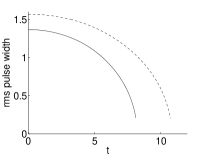
b)

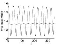
Figure 1: Rms pulse width versus time. The initial pulse has a Townes shape with mass $N=1.02N_{c}\simeq 2.77$ and radius $a_{0}=a_{c}=0.88$ (corresponding to an initial rms pulse width $a_{rms,0}=1.38$, solid line) or $a_{0}=1.0$ ($a_{rms,0}=1.57$, dashed lines). Picture a: collapse at finite time in absence of nonlinearity management. Picture b: a periodic cubic nonlinearity management $\gamma(t)=10\cos(50t)$ is applied and the pulse rms width is plotted till time $t=350$.

We have repeated the same experiments with different initial masses, to check the validity of formulas (13-14). For $N=1.04N_{c}$ (resp. $N=1.08N_{c}$), the theoretical fixed points and oscillation periods are $a_{c}=0.63$ and $T_{c}=14$ (resp. $a_{c}=0.42$ and $T_{c}=5.1$). As it can be seen in Fig. 2b, when the initial mass is significantly larger than the critical mass, the pulse first experiences a strong distortion and emits radiation. The resulting pulse is still stable, its mass is still well above the critical mass, but the fixed point and oscillation period are not well predicted by the variational analysis. If the initial mass is even larger, then this first phase leads to collapse, which shows that the stabilizing effect of the cubic nonlinearity management $\gamma(t)=10\cos(50t)$ is only efficient when the initial mass is in the range $[N_{c},1.1N_{c}]$.

a)

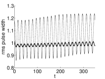
b)

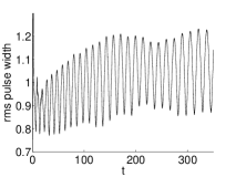
Figure 2: Rms pulse width. Picture a: $N=1.04N_{c}$, $a_{0}=0.63$ ($a_{rms,0}=0.99$, solid line), $a_{0}=0.75$ ($a_{rms,0}=1.18$, dashed lines). Picture b: $N=1.08N_{c}$, $a_{0}=0.5$ ($a_{rms,0}=0.79$, solid line).

We now prove the robustness of the solution of the CQ NLSE driven by cubic nonlinearity management with respect to the initial pulse shape. More exactly, we show that a stable solution can be obtained with an initial pulse profile which is significantly different from the Townes profile. The important conditions that have to be satisfied by the initial pulse is that its mass should be just above the critical mass corresponding to the input pulse profile, and that its initial radius should be chosen in the vicinity of the fixed point. These conditions are imposed by the analysis of Eq. (8), and they are confirmed by numerical simulations. Let us consider an arbitrary pulse shape $Q$. The critical mass is then $N_{c}=\sqrt{(3D_{1})/(D_{3}\chi)}$ and the fixed point in presence of nonlinearity management is $a_{c}=2\sqrt{2}\sqrt{D_{4}/D1}N/\sqrt{(N/N_{c})^{2}-1}$, with the period $T_{c}=(4\sqrt{2}\pi D_{4}/D_{1}^{3/2})\sigma^{2}N^{2}/[(N/N_{c})^{2}-1]^{3/2}$. A stable solution of the managed CQ NLS equation can be obtained by injecting a pulse with shape $Q$ not too far from the Townes soliton, with a mass just above $N_{c}$ and a radius close to $a_{c}$. In the case of the Gaussian ansatz $Q(x)=\exp(-x^{2}/2)$, we have $D_{1}=1$, $D_{2}=\sqrt{2/\pi}$, $D_{3}=2/(\sqrt{3}\pi)$, and $D_{4}=1/(3\sqrt{3}\pi)$. We report in Fig. 3 the results of numerical simulations carried out with $\chi=1$ so the critical mass is $N_{c}\simeq 2.86$. We use the same management as above. In a first phase ($t<20$), the pulse emits radiation and its shape converges to the one of the Townes soliton. A similar phenomenon has been observed in numerical simulations carried out in Perez for the 2D cubic NLSE with cubic nonlinearity management. After this transition period, the soliton width experiences oscillations around the fixed point with an oscillation period close to the theoretical value.

a)

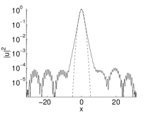
b)

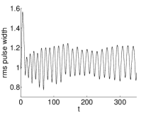
Figure 3: Dynamics of a Gaussian pulse with initial mass $N=1.02N_{c}=2.92$ and radius $a_{0}=a_{c}=1.4$ ($a_{rms,0}=0.99$). Picture a: pulse profile at time $t=350$ (solid line) compared to the input Gaussian profile (dashed lines). Picture b: rms pulse width versus time.

We finally study the stabilization induced by random nonlinearity management. Accordingly we now consider that $\gamma_{1}$ is a zero-mean stationary random process. Considering Eqs. (11-12), it can be seen that the important process is actually $\Gamma_{1}(t)=\int_{0}^{t}\gamma_{1}(s)ds$, and it is critical that this process does not grow in a diffusive manner, which would mean that cubic nonlinearity accumulates. This condition is fulfilled if $\gamma_{1}$ is the derivative of a stationary random process, or if we apply a pinning scheme. This technique was first introduced by Chertkov02 to compensate for accumulated fiber dispersion. The periodic insertion of additional pieces of fiber with well controlled lengths and dispersion values was found to prevent from pulse deterioration. The pinning method can be applied to compensate for accumulated cubic nonlinearity as well. In Fig. 4 we show that random cubic nonlinearity management stabilizes a Townes soliton in a manner similar to a periodic management. However, we can detect a very slow spreading out, whose origin can be explained by the imperfect compensation of the accumulated nonlinearity by the pinning scheme.

Figure 4: Rms pulse width versus time. The initial pulse has a Townes shape with mass $N=1.02N_{c}\simeq 2.77$ and radius $a_{0}=a_{c}=0.88$ ($a_{rms,0}=1.38$, solid line) or $a_{0}=1.0$ ($a_{rms,0}=1.57$, dashed lines). We apply a random cubic nonlinearity management $\gamma(t)=10m(50t)$ where $m$ is zero-mean stationary random process with a unit coherence time compensated by a pinning scheme.

In conclusion we have analyzed the stabilizing role of the strong management of the cubic nonlinearity in the 1D cubic-quintic NLSE. We have proved that the averaged CQ NLSE, in a dramatic distinction from the non-modulated system, supports stable solutions beyond the critical mass. In particular the quintic Townes soliton, which is unstable in the non-modulated system, becomes stable in presence of strong nonlinearity management if its width lies in the vicinity of some fixed point. This fixed point and the associated oscillation frequency are well predicted by the variational approach applied to the averaged CQ NLSE. We have also developed and applied a modified variational approach to the CQ NLSE with strong management, which gives the same values for the parameters of the stabilized soliton. We have checked that a random management is also stabilizing, if we take care to select a random process whose cumulative values are small. These results can be applied for the search of nonlinearity managed solitons in double-doped optical fibers and BECs with three-body interactions.

References

- (1) C. Sulem and P.-L. Sulem, The Nonlinear Schrödinger Equation (Springer, New York, 1999).
- (2) V. Zharnitsky, E. Grenier, C. K. R. T. Jones, and S. K. Turitsyn, Physica D 152, 794 (2001).
- (3) F. Kh. Abdullaev, B. B. Baizakov and M. Salerno, Phys. Rev. E 68, 066605 (2003).
- (4) L. Berge, V. K. Mezentsev, J. J. Rasmussen, P. L. Christiansen, and Y. B. Gaididei, Opt. Lett. 25, 1037 (2000).
- (5) I. Towers and B. A. Malomed, J. Opt. Soc. Am. B 19, 537 (2002).
- (6) F. Kh. Abdullaev, J. G. Caputo, R. A. Kraenkel, and B. Malomed, Phys. Rev. A 67, 013605 (2003); F. Kh. Abdullaev, E. N. Tsoy, B. Malomed and R. A. Kraenkel, Phys. Rev. A 68, 0536606 (2003).
- (7) H. Saito and M. Ueda, Phys. Rev. Lett. 90, 040403 (2003).
- (8) G. Montesinos, V. M. Perez-Garcia, and P. Torres, Physica D 191, 193 (2004); G. Montesinos, V. M. Perez-Garcia, and H. Michinel, Phys. Rev. Lett. 92, 133901 (2004).
- (9) H. Saito and M. Ueda, Phys. Rev. A 70, 053610 (2004).
- (10) S. Adhikari, Phys. Rev. A 69, 063613 (2004).
- (11) C. De Angelis, IEEE J. Quant. Electron. 30, 818 (1994).
- (12) F. Kh. Abdullaev, A. Gammal, L. Tomio, and T. Frederico, Phys. Rev. A 63, 043604 (2001).
- (13) W. Xhang, E. M. Wright, H. Pu, and P. Meystre, Phys. Rev. A 68, 023605 (2003).
- (14) S. Inouye, M. R. Andrews, J. Stenger, H. J. Miesner, D. M. Stamper-Kurn, and W. Ketterle, Nature 392, 151 (1998).
- (15) D. E. Pelinovsky, P. G. Kevrekidis, D. J. Frantzeskakis, and V. Zharnitsky, Phys. Rev. E 70, 047604 (2004).
- (16) V. Zharnitsky and D. Pelinovsky, Chaos 15, 1 (2005).
- (17) D. Anderson, Phys. Rev. A 27, 3135 (1983).
- (18) B. A. Malomed, Prog. Opt. 43, 69 (2002).
- (19) M. Chertkov, I. Gabitov, P. M. Lushnikov, J. Moeser, and Z. Toroczkai, J. Opt. Soc. Am. B 19, 2538 (2002).