A new approach to partial synchronization in globally coupled rotators

Abstract

We develop a formalism to analyze the behaviour of pulse–coupled identical phase oscillators with a specific attention devoted to the onset of partial synchronization. The method, which allows describing the dynamics both at the microscopic and macroscopic level, is introduced in a general context, but then the application to the dynamics of leaky integrate-and-fire (LIF) neurons is analysed. As a result, we derive a set of delayed equations describing exactly the LIF behaviour in the thermodynamic limit. We also investigate the weak coupling regime by means of a perturbative analysis, which reveals that the evolution rule reduces to a set of ordinary differential equations. Robustness and generality of the partial synchronization regime is finally tested both by adding noise and considering different force fields.

I Introduction

Understanding the behavior of networks of dynamical units is a very important subject of research in various contexts such as information processing in the brain, or metabolic systems. Given the richness of the observed phenomenology and the relevance of many different ingredients (e.g., the topology of the connections, the presence of disorder and of delayed interactions), it is very instructive to consider even simple setups in the perspective of identifying the hopefully few mechanisms responsible for the main general phenomena. Here, we focus our attention on a type of collective behavior arising in globally coupled identical systems. The first evidence of collective behavior dates back to the 70’s, when it was proven that a nonzero mean field may spontaneously arise in an ensemble of particles stochastically moving in a bistable potential KS75 . Later, it was numerically shown that macroscopic periodic dynamics appears in coupled stochastic BCM87 as well as chaotic (Rössler) oscillators PRK96 , while the first experimental evidence was found in Josephson–junction arrays WCS96 . Collective behaviour may also arise in the presence of quenched disorder as revealed by the Kuramoto model K84 , introduced to explain the onset of synchronization in an ensemble of different units Kbook . Over the years it has been discovered that collective dynamics can be also chaotic, as found in globally coupled maps K90 and oscillators GHSS92 .

Here we investigate “partial synchronization” (pS), a little known phenomenon discovered in pulse–coupled, leaky integrate-and-fire (LIF) neurons V96 . In this regime, the mean field exhibits a periodic dynamics which, at variance with other contexts, arises in the absence of any synchronization between the single units which behave quasi-periodically. pS arises from the destabilization of a regime characterized by a constant mean field and a periodic behaviour of the single elements, their phases being equispaced. This “homogeneous regime” has been found in many different contexts such as Josephson devices HB87 , multi-mode lasers WBJR90 and electronic circuits AKS90 . By following Ref. NW92 , it is now called “splay state” and its microscopic stability properties have been studied quite in detail in SM93 . Since splay states are rather general, it is reasonable to expect that the transition to pS can be observed in a wide class of systems too. In fact, the preliminary evidence of pS found in Hindmarsh-Rose neurons and van der Pol oscillators PR confirms such expectations and poses the question of understanding the general conditions for the onset of pS.

In order to unravel this point, we develop a new formalism that allows treating pulse coupled oscillators and establishes a possible basis for an extension to different coupling schemes. The approach is introduced in a general framework to show the potentiality of the method, but the resulting delayed equations are analyzed only in the specific case of LIF neurons, since in this case a simple and explicit expression is available for one of the relevant variables: the “finite-time” Lyapunov exponent $\Lambda$. Furthermore, in the attempt of identifying the minimal model able to describe the onset of pS, we have explored both analytically and numerically the weak coupling limit, showing that a perturbative expansion allows reducing the delayed to ordinary equations. The persistence of the transition to pS for an arbitrarily small coupling strength paves the way towards more general setups. A further promising indication is given by the numerical observation that pS arises also for continuous force fields, which again suggests that the phenomenon is more general than initially conjectured V96 . Finally, we have added noise to the single neuron dynamics, finding that the macroscopic oscillations persist, though with a smaller amplitude.

II Modelling identical rotators

The investigation of globally coupled systems requires setting up a suitable (nonlinear) self-consistent approach. A much used approach to describe the collective behaviour of neural networks is dynamical mean field T93 ; GV93 ; G95 ; B99 . Here, in the absence of noise and of microscopic chaos, there is no justification a priori for coarse-graining and indeed the transition to pS can be observed already in ensembles of finitely many oscillators V96 and can thus also be viewed as a bifurcation. It is therefore desirable to develop a formalism to capture both micro- and macro-scopic features. We start from the crossing-times as they are the most suitable variables to characterize splay states. Our approach can, in fact, be viewed as an extension of the method followed in Ref.AV93 , where pseudo-crossing times have been introduced with reference to the steady dynamics. On the other hand, it is fair to recognize that the final model equations are equivalent to those obtained by implementing a dynamical mean field approach, when the latter is applicable. This implies that in the present context one can smoothly go from the microscopic to the macroscopic level.

We consider an ensemble of $N$ phase oscillators (i.e. rotators), each one characterized by the phase $\phi_{i}$, $i=0,\ldots N-1$ which evolves according to the equation

$$\dot{\phi}_{i}=F(\phi_{i},E(t))$$ (1)

where $E$ is a suitable mean field whose dynamics depends homogeneously on all the $\phi_{i}$ in a way that is not crucial for the present discussion. The force field $F(\phi,E)$ is assumed to be positive and periodic in $\phi$ with period 1, but it can be discontinuous as, e.g., a sawtooth function (this is indeed the case considered in the next section). We start defining a suitable Poincaré section, by introducing a threshold $\overline{\phi}$, which, without loss of generality, is set in $\phi=1$. Let then $t_{m}$ and $i(m)$ denote, respectively, the $m$th crossing time ($m=1,\ldots,\infty$) of the threshold and the corresponding rotator crossing the threshold. Once the labels $i$ are ordered in such a way that $\phi_{i+1}<\phi_{i}$, it follows that $i(m+N)=i(m){\rm mod}~{}N$ $i.e.$, the same oscillator crosses the threshold at time $t_{m}$ and $t_{m+N}$.

The core of the approach consists in deriving an equation linking $\delta t_{m}\equiv t_{m+1}-t_{m}$ with $\delta t_{m-N}$ in the limit of large $N$. Simple arguments show that, up to higher-order corrections in $1/N$,

$$\hskip-56.9055pt\delta t_{m}=\frac{\delta\phi_{i(m)}(t_{m})}{F(1,E(t_{m}))}\frac{\delta\phi_{i(m)}(t_{m-N})}{F(1,E(t_{m}))}{\rm e}^{\Lambda(\{E\})T_{m}}=\delta t_{m-N}\frac{F(0,E(t_{m-N}))}{F(1,E(t_{m}))}{\rm e}^{\Lambda(\{E\})T_{m}}$$ (2)

where $\delta\phi_{j}\equiv\phi_{j}-\phi_{j+1}$ (here $j$ is meant modulo $N$), while $T_{m}=t_{m}-t_{m-N}$ is the interval between two consecutive threshold crossings of the same oscillator; finally, $\Lambda(\{E\})$ is the finite-time Lyapunov exponent for a trajectory starting at time $t_{m-N}$ in $\phi=0$ and ending at time $t_{m}$ in $\phi=1$, and thus, in general, depends on the dynamics of the field $E$. The first and last equalities in the above equation state simply that the temporal separation is equal to the phase separation divided by the instantaneous velocity. The middle equality follows from the observation that, being $\delta\phi_{i(m)}$ a small quantity, it evolves according to the linearized dynamics. In view of the possible existence of a discontinuity in the force field, we carefully distinguish between the $\phi$ value just before ($\phi=1$) and after $(\phi=0$) the threshold crossing.

If the crossing-time distribution is smooth (this assumption can be verified a posteriori by integrating the resulting model), then $\delta t_{m}$ has to be of the order of $1/N$ and one can accordingly introduce the “instantaneous” flux

$$\pi(t)\equiv\frac{1/N}{\delta t_{m}},$$ (3)

where we have dropped the subscript $m$ in the l.h.s. as in the limit $N\to\infty$, the time variable becomes again continuous. Accordingly, Eq. (2) simplifies to

$$\pi(t)=\pi(t-T)\frac{F(1,E(t))}{F(0,E(t-T))}{\rm e}^{-\Lambda(\{E\})T}\,,$$ (4)

where the time interval $T$ is self-consistently determined from the integral expression

$$\int_{t-T(t)}^{t}dt^{\prime}\pi(t^{\prime})=1\quad,$$ (5)

expressing the condition that from time $t-T(t)$ to time $t$, all oscillators cross the threshold. An equivalent and more appealing equation is obtained by evaluating the time derivative of Eq. (5), namely

$$\dot{T}=1-\frac{\pi(t)}{\pi(t-T)}.$$ (6)

In order to complete the derivation of a closed set of equations, it is necessary to include the mean field dynamics. In the context of pulse coupled systems, this can be easily done, since $E$ is, by definition, the linear superposition of the pulses emitted by the single oscillators whenever they reach a threshold that, without loss of generality, can be assumed to coincide with $\overline{\phi}$. Accordingly, the mean field satisfies a linear differential equation of the type

$${\mathcal{L}}(E,\dot{E},\ddot{E},\ldots)=\pi(t),$$ (7)

where the firing rate $\pi(t)$ is nothing but the previously introduced instantaneous flux, while the structure of the operator $\mathcal{L}$ can be determined by imposing that the corresponding Green function coincides with the assumed shape of the emitted pulses. This completes the derivation of the final equations that are given by Eqs. (4,6,7). The model combines properties of discrete (Eq. (4)) and continuous (Eqs. (6,7)) time systems, besides involving a time-dependent self-adjusting delay. Except for the first property, its structure resembles that of threshold delay equations LER01 introduced, e.g., in epidemiology and immunology (see SK92 for a similar model).

III An example: LIF neurons

In this section we specifically refer to the ensemble of LIF neurons studied already in Ref. V96 . In this case, $\phi$ corresponds to the (adimensional) membrane potential which evolves according to the force field

$$F(\phi,E)=a+\lambda(1-\phi)+gE(t)\,,$$ (8)

where $g$ is the coupling constant, while $a$ and $\lambda$ determine the dependence of the force field on the potential $\phi$. If $\phi$ reaches the threshold $\overline{\phi}=1$ at time $t_{0}$, a pulse $p(t-t_{0})$ is emitted (and received by all neurons), while the potential is reset to 0. The resetting makes it legitimate to interpret $\phi$ as a phase variable, since one can formally extend $\phi$ to the whole real axis by identifying $\phi$ with $\phi+1$ and thereby see the evolution as a continuous process. Paying attention to the discontinuities present in the force field, Eq. (4) writes as

$$\pi(t)=\pi(t-T)\frac{a+gE(t)}{a+\lambda+gE(t-T)}{\rm e}^{\lambda T}\quad,$$ (9)

where we have also taken into account that, because of the linearity of the force field, the Lyapunov exponent $\Lambda$ appearing in Eq. (4) is equal to $-\lambda$ independently of the $E$ dynamics.

As for the mean field, if we assume that the single pulse shape is $p(t-t_{0})=\alpha^{2}(t-t_{0}){\rm e}^{-\alpha(t-t_{0})}$, one finds that $E$ satisfies the equation V96

$$\ddot{E}+2\alpha\dot{E}+\alpha^{2}E=\alpha^{2}\pi\quad.$$ (10)

As a result, the model reduces to the set of equations (6,9,10). For a small enough $\alpha$ value, the dynamics converges to a fixed point. Since all neurons sequentially cross the firing threshold, the translational invariance of a fixed point automatically implies a uniform distribution of the phase differences, that is the distinguishing feature of splay states. A tedious but strightforward linear stability analysis proves that the splay state destabilizes at the critical value already identified in V96 , where a Hopf bifurcation signals theonset of a collective periodic behaviour, i.e. of pS.

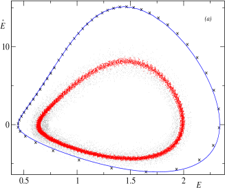
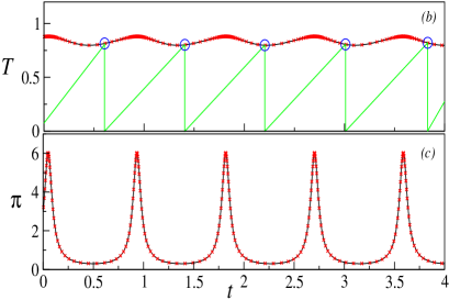
Figure 1: Comparison between the initial model for $N=100$ oscillators (crosses) and the set of equations (6,9,10) (solid line) for $a=0.3$, $g=0.4$, $\lambda=1$ and $\alpha=9$. The representation in the phase space $(\dot{E},E)$ is plotted in panel (a), while the time evolution of $T$ and $\pi$ is drawn in (b) and (c). The dots in panel (a) correspond to simulations performed in the presence of additive uniformly distributed noise of width $\sigma=0.025$ (the wider band corresponds to $N=200$, while the other to $N=4000$). Finally, a geometric procedure for reconstructing the single neuron firing times is plotted in (b).

In Fig. 1 we present the outcome of numerical simulations carried on in the pS regime. First of all, notice that the results are basically indistinguishable from those of the original set of equations, as they should. It is then instructive to look at $T(t)$, since it provides a bridge with the microscopic description. In fact, if we denote with $t_{n}[i]$ the time when the $i$th neuron emits a spike (i.e., it crosses the threshold $\overline{\phi}$), $T(t_{n}[i])$ represents the last inter-spike interval (ISI) of the very same neuron and all past spike times are obtained by simply iterating the recursive formula

$$t_{n-1}[i]=t_{n}[i]-T(t_{n}[i]).$$ (11)

Geometrically, the implemetation of this formula corresponds to the following procedure (see Fig. 1b): given the point $(t_{n},T(t_{n}))$, move down along a straight line of slope $1$ until the $t$-axis is reached at the time $t_{n-1}$ and then vertically up until the $T$-curve is hit. Considering that $T(t)$ is a positive definite periodic function, Eq. (11) describes nothing but the evolution equation of a periodically forced oscillator, so that one expects the onset of locking phenomena. However, it appears that the self-generated $T$ dynamics does not exhibit any such locking, even when the ratio of the two frequencies is rational. This remarkable feature remains unexplained.

Another peculiarity of pS is that the single–neuron ISI differs from (it is always smaller than) the period of the macroscopic dynamics. Interestingly enough, this is the distinguishing feature of slowly oscillating periodic solutions already found in equations with state-dependent delay LER01 . Qualitatively, the phenomenon can be clarified by noticing that neurons tend to bunch together, but, at the same time, those neurons lying in the front of the cluster escape away, while those reaching the back get stuck. This justifies the name “partial synchronization” attributed to this phenomenon.

IV Perturbative analysis

Upon exploring the parameter plane $(\alpha,\lambda)$, we have discovered that pS can be observed for arbitrarily small $\lambda$-values. As a result, one can hope to shed further light on this phenomenon, by developing a perturbative analysis. This is not easy, because the limit case $\lambda=0$ is degenerate, as Eq. (9) is satisfied by any periodic function $\pi(t)$. In fact, in this limit, there are no effective interactions among the oscillators and their distribution does not change in time, whatever the initial choice is. The only constraints are given by Eq. (10), which allows determining $E(t)$ and Eq. (5), which fixes the period $P=(1-g)/a$. Thus, exactly for $\lambda=0$, pS cannot arise, since the periodicity of the single oscillators necessarily coincides with the collective periodicity. However, as soon as $\lambda>0$, $T$ can differ from the period $P$, $T(t)=P+\lambda\tau(t)$. Accordingly, for a generic function $u(t)$ periodic of period $P$, one can write

$$u(t-T)=u(t-\lambda\tau)=u(t)-\lambda\tau\dot{u}(t)+O(\lambda^{2}).$$ (12)

By introducing this expansion into the model equations (9,10), one obtains, up to first order in $\lambda$,

$$\dot{\tau}=-P+\frac{1-g\tau\dot{E}}{a+gE}$$ (13)

$$\ddot{E}+2\alpha\dot{E}+\alpha^{2}E=\alpha^{2}\frac{C}{\tau}.$$ (14)

The same procedure, when applied to Eq. (6), implies that $\pi\tau=C$, where $C$ is a constant of motion, so that the model reduces to a simple set of ordinary differential equations in a three dimensional space ($E$, $\dot{E}$ and $\tau$ being the relevant variables). The a priori unknown parameter $C$ must be determined self-consistently by imposing that the integral of $\pi=C/\tau$ over the period $P$ is equal to $1$. By numerically integrating the above set of equations, we find a self-consistent solution above a suitable critical $\alpha$-value. The corresponding collective behaviour is plotted in Fig. 2 for different $\alpha$-values.

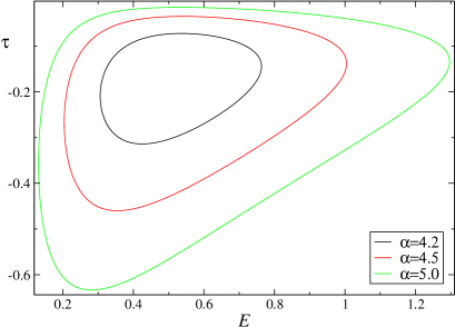
Figure 2: The amplitude of $E$ and $\tau$ decreases as one approaches $\alpha_{c}=4.055(8)$ (the critical point for $\lambda=0.001$ and $g=0.4$). The transition is thus a supercritical Hopf bifurcation.

V Conclusions and perspectives

In order to test the robustness of the pS regime, we have performed some further studies both to verify whether the discontinuity in the force field is a necessary condition and to explore the stability against the addition of external noise. The simplest way to introduce a continuous force field is by adding a branch $F^{\prime}(\phi)=a+\lambda^{\prime}\phi+E$ (with $\phi<\phi_{0}=\lambda/(\lambda^{\prime}-\lambda)$) to Eq. (8) which is now restricted to $\phi>\phi_{0}$. It is in principle possible to follow the same approach that has led to Eq. (9), but here we limit ourselves to mentioning the result of our numerical simulations, namely that for $\lambda^{\prime}>\approx 14\lambda$, the continuous model keeps exhibiting a transition to pS. Finally, we have numerically analysed the original model, under the further action of a zero-average uniformly distributed noise of width $\sigma=0.025$ for $N=200$ and $4000$. The results, plotted in Fig. 1, show that the collective behaviour, though depressed by the noise action, persists. In fact, the transversal fuzziness appears to decrease with the number $N$ of oscillators as $1/\sqrt{N}$.

In the second section we have obtained a closed set of equations to treat identical pulse-coupled rotators. The main obstacle towards specific applications is the need to express the finite-time Lyapunov exponent in Eq. (4) in terms of the other relevant variables. This seems to be only a technical problem, that we have indeed recently solved for generic sinusoidal fields prog . On the other hand, it is less clear how to incorporate the effect of noise and disorder. In this respect, a close comparison with the dynamical mean field approach should be very helpful, since noise can be easily handled by the latter one, while our method is more open to the treatment of generic force fields.

We thank an unknown referee for having drawn to our attention a similar bifurcation found in systems with variable time delay.

References

References

- (1) Kometani K and Shimizu H 1975 J. Stat. Phys. 13 473; Desai R C and Zwanzig R 1978 J. Stat. Phys. 19 1
- (2) Bonilla L L Casado J M and Morillo M 1987 J. Stat. Phys. 48 571
- (3) Pikovsky A S Rosenblum M G and Kurths 1996 J. Europhys. Lett. 34 165
- (4) Wiesenfeld K Colet P and Strogatz S H 1996 Phys. Rev. Lett. 76 404
- (5) Kuramoto Y 1984 Prog. Theor. Phys. Supp. 79 223
- (6) Kuramoto Y 1984 Chemical Oscillations, Waves and Turbulence, Springer-Verlag, New York
- (7) Kaneko K 1990 Phys. Rev. Lett. 65 1391; Pikovsky A S and Kurths J 1994 Phys. Rev. Lett. 72, 1644; Shibata T Chawanya T and Kaneko K 1999 92 4424
- (8) Golomb D Hansel D Shraiman B and Sompolinsky H 1992 Phys. Rev. A 45, 3516; Hakim V and Rappel W 1992 Phys. Rev. A 46 R7347; Nakagawa N and Kuramoto Y 1993 Prog. Theor. Phys. 89 313
- (9) van Vreeswijk C 1996 Phys. Rev. E 54 5522
- (10) Hadley P and Beasley M R 1987 Appl. Phys. Lett. 50 621
- (11) Wiesenfeld K Bracikowski C James G and R. Roy 1990 Phys. Rev. Lett. 65, 1749
- (12) Ashwin P King G P and Swift J W 1990 Nonlinearity 3, 585
- (13) Nichols S and Wiesenfeld K 1992 Phys. Rev. A 45 8430
- (14) Strogatz S H and Mirollo R E 1993 Phys. Rev. E 47 220
- (15) Pikovsky A and Rosenblum M, private communication
- (16) Treves A 1993 Network 4 256
- (17) Gerstner W and van Hemmen L 1993 Phys. Rev. Lett. 71 312
- (18) Gerstner W 1995 Phys. Rev. E 51 738
- (19) Bressloff P C Phys. Rev. E 60 2160
- (20) Abbott L F and van Vreeswijk C 1993 Phys. Rev. E 48 1483
- (21) Luzyanina T Engelborghs K Roose D 2001 Int. J. Bifur. Chaos 11 737
- (22) Smith H L and Kuang Y 1992 Contemp. Math. 129 153
- (23) Mohanty P K and Politi A, work in progress