Classical limit of transport in quantum kicked maps

Abstract

We investigate the behavior of weak localization, conductance fluctuations, and shot noise of a chaotic scatterer in the semiclassical limit. Time resolved numerical results, obtained by truncating the time-evolution of a kicked quantum map after a certain number of iterations, are compared to semiclassical theory. Considering how the appearance of quantum effects is delayed as a function of the Ehrenfest time gives a new method to compare theory and numerical simulations. We find that both weak localization and shot noise agree with semiclassical theory, which predicts exponential suppression with increasing Ehrenfest time. However, conductance fluctuations exhibit different behavior, with only a slight dependence on the Ehrenfest time.

I Introduction

According to Ehrenfest’s theorem, the expectation values of the position and momentum of an electron obey classical equations of motion. As long as the wavefunction of the electron is a wavepacket with minimal uncertainties in momentum and position, the expectation values are a good description of the quantum state. However, wavepackets disperse, and the Ehrenfest theorem looses its relevance after a short time. In a cavity with point scatterers, which split electron wavepackets into partial waves after one scattering event, this time is simply the elastic mean free time. In a ballistic cavity with chaotic classical dynamics, this time is the so-called “Ehrenfest time” $\tau_{\rm E}$, which depends on the Lyapunov exponent $\lambda$ of the classical motion in the cavity.Zaslavsky (1981); Aleiner and Larkin (1996) For times longer than $\tau_{\rm E}$, a classical description no longer holds and the wave nature of the electrons becomes visible.

The wave nature of electrons is the cause of some striking effects that are absent in classical systems. For transport through cavities coupled to source and drain reservoirs via point contacts, these effects are weak localization, universal conductance fluctuations, and shot noise.Beenakker and van Houten (1991a) In the limit that transport through cavities is ergodic (dwell time in the cavity is much longer than the time of flight through the cavity), the signatures of quantum transport are ‘universal’, independent of the cavity size and shape, and of the fact whether electron motion inside the cavity is ballistic and chaotic or diffusive, with repeated scattering off impurities with size smaller than the electron wavelength. Random matrix theory provides a unified theoretical description of weak localization, universal conductance fluctuations, and shot noise in ballistic or diffusive cavities.Beenakker (1997)

If the electron motion is diffusive, the dynamics is fully quantum mechanical already at times much shorter than the time $\tau_{\rm erg}$ required for ergodic exploration of the cavity’s phase space. For ballistic cavities this is true in most practical applications as well — the Ehrenfest time $\tau_{\rm E}$ usually does not exceed the time of flight through the cavity — but there is no fundamental reason why $\tau_{\rm E}$ always has to be small. The case of large Ehrenfest times is of theoretical interest, as it is one of very few regimes in parameter space in which one can observe differences between signatures of quantum transport in ballistic chaotic and diffusive cavities.

The most prominent effects of a large Ehrenfest time are found if $\tau_{\rm E}$ is larger than the dwell time $\tau_{\rm D}$ in the cavity. If $\tau_{\rm E}\gg\tau_{\rm D}$, quantum transport is deterministic, and shot noise is suppressed.Beenakker and van Houten (1991b); Agam et al. (2000) The suppression of shot noise has been observed experimentally by varying the dwell time $\tau_{\rm D}$ of a chaotic cavity,Oberholzer et al. (2002) and numerically, using a chaotic map as a model for a chaotic cavity.Tworzydlo et al. (2003); Jacquod and Sukhorukov (2004); Jacquod and Whitney (2005) The effect of a large Ehrenfest time on weak localization was first addressed by Aleiner and Larkin.Aleiner and Larkin (1996) Their theory predicts a suppression of weak localization $\propto\exp(-\tau_{\rm E}/\tau_{\rm D})$, if classical correlations are taken into account properly.Rahav and Brouwer (2005) The same suppression was found in an independent calculation by Adagideli.Adagideli (2003) Experimental observation of the suppression of weak localization at large Ehrenfest times has been reported for transport through antidot arrays.Yevtushenko et al. (2000) No semiclassical theory for the Ehrenfest-time dependence of universal conductance fluctuations exists. However, semiclassical theories for weak localization and universal conductance fluctuations for the limit $\tau_{\rm D}\gg\tau_{\rm E}$ are essentially equal,Argaman (1995, 1996); Takane and Nakamura (1997, 1998) as are diagrammatic perturbation theories for the same phenomena in diffusive cavities, supporting the expectation that the Ehrenfest-time dependencies of weak localization and universal conductance fluctuations will be equal as well.Tworzydlo et al. (2004a)

Direct numerical simulation of the effect of a large Ehrenfest time on quantum transport through two-dimensional chaotic cavities has been problematic because of the prohibitively high computational cost of the simulations. The reason is that $\tau_{\rm E}$ depends only logarithmically on the product of the electron wavenumber $k$ and the cavity size $L$,

$$\tau_{\rm E}=\lambda^{-1}\ln kL.$$ (1)

For two-dimensional cavities, system sizes at which $\tau_{\rm E}\gtrsim\tau_{\rm D}$ cannot be simulated with present-day algorithms and processor speeds. In order to circumvent this problem, Jacquod, Schomerus, and Beenakker proposed to replace the cavity by a quantum map.Jacquod et al. (2003) The map is ’opened’, so that simulation of transport properties is possible. Although a map has a one-dimensional phase space, a chaotic map shares many characteristics of the chaotic motion in two-dimensional chaotic cavities.Stöckmann (1999) The reduced dimensionality of the map’s phase space made numerical simulations with larger Ehrenfest times possible. For an open version of the quantum kicked rotator map, numerical simulations were reported for shot noise,Tworzydlo et al. (2003); Jacquod and Sukhorukov (2004); Jacquod and Whitney (2005) weak localization,Tworzydlo et al. (2004b); Rahav and Brouwer (2005) and universal conductance fluctuations.Jacquod and Sukhorukov (2004); Tworzydlo et al. (2004c, a) Simulation results for shot noise were in good agreement with the predictions of the semiclassical theory.Agam et al. (2000) However, for conductance fluctuations, no dependence on $\tau_{\rm E}$ was found, despite the fact that Ehrenfest times larger than the dwell time were considered. footnote Whereas early numerical simulations of weak localization showed no Ehrenfest-time dependence,Tworzydlo et al. (2004b) we showed that there is a systematic decrease of the weak localization correction to the conductance upon increasing $\tau_{\rm E}$, consistent with the semiclassical theory.Rahav and Brouwer (2005)

The main technical innovation that allowed us to detect a systematic decrease of the weak localization correction upon increasing the Ehrenfest time is that we looked at time-resolved numerical simulations: The map’s time evolution is truncated after a time $t_{0}$, and weak localization, conductance fluctuations, and shot noise are monitored as a function of $t_{0}$.Rahav and Brouwer (2005) This procedure has two advantages. First, it allows the ensemble average over the quasienergy $\varepsilon$ to be done analytically. (See Sec. II for technical details.) This made it possible to consider significantly larger ensembles than considered previously. Second, monitoring quantum corrections as a function of the ‘truncation time’ $t_{0}$ allows us to determine the minimal time after which quantum corrections can occur. In the semiclassical theory, quantum interference requires a minimal wavepacket to be split and reunited, which takes a minimal time $2\tau_{\rm E}$. A schematic diagram drawing relevant semiclassical trajectories for weak localization and conductance fluctuations is shown in Fig. 1. (The diagram for conductance fluctuations is taken from Ref. Takane and Nakamura, 1998 and modified to contain the effect of a finite Ehrenfest time.) Not being a quantum interference effect, shot noise only requires wavepackets to be split, which happens after a time $\tau_{\rm E}$. Comparison of the time when quantum effects appear (the ‘onset time’) and the rate of suppression of quantum effects as the Ehrenfest time $\tau_{\rm E}$ is increased, thus provides a quantitative test of the semiclassical theory. With such a quantitative test of the semiclassical theory, accurate simulations performed at smaller Ehrenfest times can still be meaningful.

Figure 1: Schematic drawing of relevant trajectories for weak localization (a), conductance fluctuations (b), and shot noise (c). The letters “L” and “R” refer to the left and right contacts to the cavity, respectively. The trajectories shown in panel (a) are for the weak localization to the transmission $T$; the trajectories shown in panel (b) are for the covariance $\mbox{cov}(R_{\rm L},R_{\rm R})$ of reflections from the left and right contacts. Both weak localization and conductance fluctuations require a minimal dwell time of $2\tau_{\rm E}$. Shot noise requires a minimal dwell time $\tau_{\rm E}$ only.

In this paper, we present detailed results of such time-resolved numerical simulation for weak localization, conductance fluctuations, and shot noise. For all three quantum effects, we analyze their Ehrenfest-time dependence (without truncation of the time evolution) and the onset times (obtained from simulations with truncation of the time evolution). The simulation results are presented in Sec. II, together with the predictions of random matrix theory for time-resolved transport through open quantum maps. Whereas we confirm our earlier conclusion that the numerical simulations for weak localization show a suppression $\propto\exp(-\tau_{\rm E}/\tau_{\rm D})$, consistent with the semiclassical theory, we find that simulations for conductance fluctuations show a very small increase if $\tau_{\rm E}$ is increased, the effect being small enough to be consistent with the simulation data reported in the literature.Jacquod and Sukhorukov (2004); Tworzydlo et al. (2004c, a) The onset times for conductance fluctuations are more than a factor two smaller than the onset times for weak localization, which is incompatible with the notion that conductance fluctuations arise as wavepackets are split and reunited.

A second goal of this paper is to show how classical correlations are taken into account in the semiclassical theory of Ref. Aleiner and Larkin, 1996. The importance of classical correlations — no quantum diffraction takes place to or from classical trajectories with classical dwell time shorter than the Ehrenfest time — was pointed out in the analysis of simulation data for the quantum kicked rotator, most notably the simulations for shot noise.Tworzydlo et al. (2003) The original version of the semiclassical theory,Aleiner and Larkin (1996) which did not include these correlations, predicted a suppression of weak localization $\propto\exp(-2\tau_{\rm E}/\tau_{\rm D})$. It is only after accounting for the classical correlations that the proper exponential decay $\propto\exp(-\tau_{\rm E}/\tau_{\rm D})$ is recovered. (Classical correlations are taken into account correctly in the semiclassical theory of shot-noise suppression at large Ehrenfest times.Agam et al. (2000)) In addition it is demonstrated that this semiclassical theory is unitary, i.e., that no probability is lost. Our discussion of the semiclassical theory for weak localization can be found in Sec. III. We conclude in Sec. IV.

II Time resolved transport in open quantum maps

Despite their different dimensionality, chaotic quantum maps are believed to have the same phemonology as (closed) chaotic cavities,Fishman et al. (1982); Altland and Zirnbauer (1996); Borgonovi et al. (1996); Frahm (1997) provided one restricts attention to the “universal limit” of times longer than the “ergodic time”. (The “ergodic time” is the time required to explore the phase space.) Open kicked quantum maps have been used as a model for transport through chaotic cavities,Jacquod et al. (2003) because maps allow to simulate systems with many transport channels with relatively small computational effort. For short times, qualitative differences between maps and cavities exist, however, because the time evolution in maps is discrete, whereas the time evolution in cavities is not.

Quantum maps operate on a finite state vector $\psi$ of dimension $M$. In the context of the quantum kicked rotator these states are discrete quasimomentum states or, alternatively, positions on a lattice with periodic boundary conditions. In the language of a cavity, the elements of $\psi$ can be thought of as points on the cavity boundary. The time evolution of such maps is discrete, and given by the Floquet operator

$$\psi(t+1)={\cal F}\psi(t).$$ (2)

For the kicked rotator, this type of dynamics is relatively easy to simulate numerically, which is why it is used to numerically model quantum interference corrections at large Ehrenfest times.

In order to study transport, the system has to be opened. Hereto two consecutive sets of $N_{\rm L}$ and $N_{\rm R}$ elements $\psi$ are chosen that corresponds to two ‘leads’.Jacquod et al. (2003) The initial condition for a transport simulation corresponds to $\psi$ localized at one of the ‘lead’ points. Escape from the cavity is modeled by recording the amplitude of $\psi$ at the lead points at time $t$ and setting $\psi$ to zero afterwards. Formally, this corresponds to the constructionBrouwer et al. (1999); Fyodorov and Sommers (2000); Ossipov et al. (2003); Tworzydlo et al. (2003)

$$S(\varepsilon)=P\left[1-e^{i\varepsilon}{\cal F}Q\right]^{-1}e^{i\varepsilon}{\cal F}P^{T},$$ (3)

where $S$ is the scattering matrix corresponding to the map, $\varepsilon$ is quasienergy, $P$ is a $(N_{\rm R}+N_{\rm L})\times M$ matrix projecting on the sites corresponding to the left (L) and right (R) contacts, and $Q=1-P^{T}P$. The conductance coefficients $G_{\rm LL}$, $G_{\rm RL}$, $G_{\rm LR}$, and $G_{\rm RR}$ are defined as

$$G_{\rm RL} \equiv \mbox{tr}\,SC_{\rm L}S^{\dagger}C_{\rm R},$$

$$G_{\rm LR} \equiv \mbox{tr}\,SC_{\rm R}S^{\dagger}C_{\rm L}$$

$$G_{\rm LL} \equiv \mbox{tr}\,SC_{\rm L}S^{\dagger}C_{\rm L}-N_{\rm L},$$

$$G_{\rm RR} \equiv \mbox{tr}\,SC_{\rm R}S^{\dagger}C_{\rm R}-N_{\rm R},$$ (4)

where $C_{\rm R}$ projects on the channels of the right lead, whereas $C_{\rm L}$ projects on the channels of the left lead. Unitarity implies $G_{\rm RL}=G_{\rm LR}=-G_{\rm LL}=-G_{\rm RR}$. The dwell time corresponding to the map is $\tau_{\rm D}=M/(N_{\rm L}+N_{\rm R})$.

We note that, with this method of opening the map, the leads end abruptly. Such abrupt changes lead to diffraction effects, similar to diffraction from sharp corners at the lead opening of a cavity. The semiclassical contributions of some diffracting orbits of this type were calculated for closed and open cavities, see, e.g., Refs. Sieber et al., 1997; Bogomolny et al., 2000; Stampfer et al., 2005. They were found to be an important contribution to shot noise at small channel numbers $N$ for rectangular cavities.Aigner et al. (2005); Marconcini et al. (2004) However, to the best of our knowledge, the total contribution of such orbits to shot noise, weak localization, and conductance fluctuations in chaotic cavities at large $N$ are unknown. Therefore, we compare our numerical results to the existing semiclassical theory, which neglects the effects of corner diffraction.

In this section, we will study the transmission and reflection coefficients as a function of a truncation time $t_{0}$. The truncation procedure involves writing Eq. (3) as a geometric series of a time-dependent scattering matrix $S(t)$,

$$S(\varepsilon)=\sum_{t=1}^{\infty}e^{i\varepsilon t}S(t),$$ (5)

with

$$S(t)=P\left[{\cal F}Q\right]^{t-1}{\cal F}P^{T}.$$ (6)

Instead of taking the full geometric series (5), we truncate the series after time $t_{0}$,

$$S(t\leq t_{0};\varepsilon)\equiv\sum_{t=1}^{t_{0}}e^{i\varepsilon t}S(t),$$ (7)

and study transport properties as a function of $t_{0}$. Although such a truncation procedure does not represent a physical system, it allows us to get theoretical information on the times involved in quantum transport phenomena. In particular, we will verify at what truncation time weak localization and conductance fluctuations will first appear.

The quantities of interest are the ensemble-averaged conductance coefficients $G_{\rm LL}$, $G_{\rm RL}$, $G_{\rm LR}$, and $G_{\rm RR}$, with $S$ replaced by $S(t\leq t_{0})$, and the fluctuations of these coefficients. With the truncation procedure, $S$ is no longer unitary, so that one does not necessarily have that $G_{\rm RL}=G_{\rm LR}=-G_{\rm LL}=-G_{\rm RR}$. Hence, we need to consider all four conductance coefficients separately. If ${\cal F}$ is time-reversal symmetric, one still has $G_{\rm RL}=G_{\rm LR}$, and only three conductance coefficients need to be considered. For $t_{0}\gg\tau_{\rm D}$, unitarity is restored, and one conductance coefficient is sufficient.

It is also of interest to study the $t_{0}$ dependence of shot noise. This also can be done by replacing the scattering matrix by $S(t\leq t_{0})$, as was done for weak localization and conductance fluctuations. The resulting $t_{0}$-dependent Fano factor is given by Tworzydlo et al. (2003)

$$F(t_{0})=\frac{N_{\rm R}+N_{\rm L}}{N_{\rm R}N_{\rm L}}\operatorname{tr}\left[SC_{\rm R}S^{\dagger}C_{\rm L}\left(1-SC_{\rm R}S^{\dagger}C_{\rm L}\right)\right].$$ (8)

The ensemble average is taken by first averaging over the quasienergy $\varepsilon$, and then over various lead positions. The quasienergy average can be performed explicitly, see Eq. (7) above. For the fluctuations, we consider the variances of the transport coefficients, as well as covariances of different coefficients. The variances are taken with respect to the quasienergy $\varepsilon$, in order to ensure that the fluctuations are entirely of quantum origin.Tworzydlo et al. (2004c); Jacquod and Sukhorukov (2004) The variance or covariance for fluctuations with respect to $\varepsilon$ is then averaged over different lead positions. Again, having the explicit energy dependence (7) at our disposal, the calculation of the variance or covariance with respect to variations of $\varepsilon$ can be performed explicitly.

II.1 Random matrix theory of time-resolved transport

As a reference for our numerical simulations, in which we take the Floquet operator ${\cal F}$ of the quantum kicked rotator, we consider averages and fluctuations of the transport coefficients for the case that ${\cal F}$ is a random symmetric unitary matrix, taken from the circular orthogonal ensemble of random matrix theory. In the limit of large $M$, $N_{\rm L}$, and $N_{\rm R}$, which is relevant for the semiclassical limit we consider throughout this paper, such averages can be calculated using the technique of Ref. Brouwer and Beenakker, 1996. We then find

$$\langle G_{\alpha\beta}(t\leq t_{0})\rangle=\langle G_{\alpha\beta}(t\leq t_{0})\rangle_{\rm cl}+\delta G_{\alpha\beta}(t\leq t_{0})+O(M^{-2}),$$ (9)

where the indices $\alpha$ and $\beta$ can be taken to be L and R. The first term $\langle G_{\alpha\beta}(t_{0})\rangle_{\rm cl}$ is the classical average,

$$\langle G_{\alpha\beta}(t\leq t_{0})\rangle_{\rm cl}=\frac{N_{\alpha}N_{\beta}}{M}\frac{1-x^{t_{0}}}{1-x}-N_{\alpha}\delta_{\alpha\beta},$$ (10)

with $x=1-1/\tau_{\rm D}$, and $\delta G_{\alpha\beta}(t_{0})$ is the weak localization correction,

$$\delta G_{\alpha\beta}(t\leq t_{0}) = \frac{N_{\alpha}(1-x^{t_{0}})}{M(1-x)}\delta_{\alpha\beta}-\frac{N_{\alpha}N_{\beta}}{M^{2}}\left(\frac{1-x^{t_{0}}}{(1-x)^{2}}-\frac{t_{0}x^{t_{0}}}{1-x}+\frac{t_{0}(t_{0}-1)x^{t_{0}-1}}{2}\right).$$ (11)

For the covariances we find similarly in the limit of $M$, $N_{\rm R}$, $N_{\rm L}\gg 1$,

$$\langle\operatorname{cov}_{\varepsilon}\left[G_{\alpha\beta}(t\leq t_{0}),G_{\gamma\delta}(t\leq t_{0})\right]\rangle=2\frac{N_{\alpha}N_{\beta}N_{\gamma}N_{\delta}}{(N_{\rm L}+N_{\rm R}+1)^{4}}{\cal R}_{1}+2\frac{N_{\alpha}N_{\beta}}{(N_{\rm R}+N_{\rm L}+1)^{3}}\left(N_{\gamma}\delta_{\beta\delta}+N_{\gamma}\delta_{\alpha\delta}+N_{\delta}\delta_{\alpha\gamma}+N_{\delta}\delta_{\beta\gamma}\right){\cal R}_{2}\\ +2\frac{N_{\alpha}N_{\beta}}{(N_{\rm R}+N_{\rm L}+1)^{2}}\left(\delta_{\alpha\gamma}\delta_{\beta\delta}+\delta_{\alpha\delta}\delta_{\beta\gamma}\right){\cal R}_{3}+O(M^{-1}),$$ (12)

where

$${\cal R}_{1} =\frac{2x}{1+x}-2x^{t_{0}-1}\left((t_{0}+1)x^{2}+6x-t_{0}+1\right)-\frac{2x^{2t_{0}-1}}{1+x}+x^{2t_{0}-2}$$

$$\times\left(-\frac{2}{3}(1-x)^{3}t_{0}^{3}+(1-x)^{2}(1+x)t_{0}^{2}+\frac{1}{3}t_{0}(1-x)(11x^{2}+20x-1)+2x(x^{2}+5x+2)\right),$$

$${\cal R}_{2} =-\frac{x}{1+x}+2x^{t_{0}}+\frac{x^{2t_{0}-1}}{1+x}-(t_{0}+1)x^{2t_{0}-1}+(t_{0}-1)x^{2t_{0}},$$

$${\cal R}_{3} =x\left(\frac{1}{1+x}-x^{t_{0}-1}+\frac{x^{2t_{0}-1}}{1+x}\right).$$ (13)

In Eq. (12) the symbol $\mbox{cov}_{\varepsilon}$ denotes a covariance taken with respect to variations of the quasienergy only, whereas the brackets $\langle\ldots\rangle$ denote the ensemble average over ${\cal F}$.

II.2 The open quantum kicked rotator

In our numerical simulations, we take the Floquet operator ${\cal F}$ of the quantum kicked rotator map. The map is described in detail by Tworzydlo et al., see Ref. Tworzydlo et al., 2004b. The matrix elements of the Floquet operator are

$${\cal F}_{mn}=\left(XU^{\dagger}\Pi UX\right)_{mn}$$ (14)

with

$$U_{mn} =M^{-1/2}e^{2\pi imn/M},$$

$$X_{mn} =\delta_{mn}e^{-i\frac{MK}{4\pi}\cos\left(2\pi m/M+\phi\right)},$$

$$\Pi_{mn} =\delta_{mn}e^{-i\pi m^{2}/M}.$$

Here $K$ is the so called stochasticity parameter that determines the classical dynamics of the map. The region $K\gtrsim 7.5$ is associated with classically chaotic dynamics. The parameter $\phi$ determines the precise quantization of the map and has no effect on the classical dynamics. In this model the size of the matrix $M$ is even. In the simulations we set $N_{\rm R}=N_{\rm L}=N$.

We used the Floquet operator (14) to study conductance fluctuations and shot noise. The Floquet operator (14) can also be used to study weak localization using the following argument: The average conductance $\langle G_{\alpha\beta}\rangle$ consists of a classical contribution and a quantum correction,

$$\langle G_{\alpha\beta}\rangle=G_{\alpha\beta,{\rm cl}}+\delta G_{\alpha\beta}.$$ (15)

The classical contribution $G_{\alpha\beta,{\rm cl}}$ scales proportional to the channel number $N$, whereas the quantum correction has no $N$-dependence (except for a possible weak dependence on $N$ through the Ehrenfest time). The quantum correction can be extracted by comparing average conductances at $N$ channels and $2N$ channels,

$$\delta G_{\alpha\beta} \approx 2\delta G_{\alpha\beta}(N)-\delta G_{\alpha\beta}(2N)$$ (16)

$$= 2\langle G_{\alpha\beta}(N)\rangle-\langle G_{\alpha\beta}(2N)\rangle.$$

In order to avoid a spurious contribution to $\delta G_{\alpha\beta}$ from classical conductance fluctuations, we made sure that the ensemble averages for $\langle G_{\alpha\beta}(2N)\rangle$ and $\langle G_{\alpha\beta}(N)\rangle$ were taken for precisely the same classical dynamics (same values of $K$, same lead positions). This method was used previously in Ref. Rahav and Brouwer, 2005.

Alternatively, one can study weak localization by considering maps with and without time reversal symmetry. The kicked rotator map (14) has time-reversal symmetry. A simple extension of Eq. (14) that breaks time-reversal symmetry is the so-called three-kick model,Tworzydlo et al. (2004b)

$${\cal F}_{mn}=\left(X\Pi Y^{*}\Pi Y\Pi X\right)_{mn}$$ (17)

where

$$Y_{mn} =\delta_{mn}e^{i\frac{\gamma M}{6\pi}\cos\left(2\pi m/M\right)},$$

$$X_{mn} =\delta_{mn}e^{-i\frac{M}{12\pi}V(2\pi m/M)},$$

$$\Pi_{mn} =M^{-1/2}e^{-i\pi/4}e^{i\frac{\pi}{M}(n-m)^{2}}.$$

In this model $M$ is even, but not a multiple of $3$. The kick potential is given by

$$V(\theta)=K\cos\left(\pi q/2\right)\cos\theta+\frac{1}{2}K\sin\left(\pi q/2\right)\sin 2\theta,$$ (18)

where $q$ breaks the parity symmetry of the model.Blümel and Smilansky (1992) The parameter $\gamma$ plays the role of a magnetic field and breaks time-reversal symmetry. By comparing the transport for $\gamma\neq 0$ to that of $\gamma=0$ it is possible to investigate the weak localization correction as a function of time. This is the method used in Ref. Tworzydlo et al., 2004b.

The advantage of the second method is that it does not require the cancellation of classical conductances of two different systems. The disadvantage is that it involves the additional parameter $\gamma$, which itself also affects the map’s classical dynamics. However, weak localization is affected on the scale $\gamma\sim 1/N$, so that the effect on the classical dynamics can be expected to be small in the semiclassical limit $N\gg 1$.

For both models, the Ehrenfest time is given by

$$\tau_{\rm E}=\lambda^{-1}\ln N,$$ (19)

up to an $N$-independent constant. The dwell time reads

$$\tau_{\rm D}=\frac{M}{2N}.$$ (20)

II.3 Numerical results

The numerical algorithm used to iterate the maps (14) and (17) can be accelerated by using a fast Fourier transform.Tworzydlo et al. (2004c); Tworzydlo et al. (2003); Tworzydlo et al. (2004b); Ketzmerick et al. (1999) The results are computed as a function of time and not of quasienergy. This allows to truncate the series (5) at the maximal time studied, and to calculate the $\varepsilon$-averages explicitly.

Weak localization. The value of the time-reversal symmetry breaking parameter $\gamma$ at which weak localization corrections to the conductance are suppressed in the three-kick model (17) scales inversely proportional to the channel number $N$.Tworzydlo et al. (2004b) Hence, in order to compare weak localization corrections for different channel numbers, the average conductance is calculated as a function of the product $\gamma N$. Figure 2 shows the result of numerical simulations of the ensemble-averaged conductance. The ensemble average is taken over 1000 samples, choosing $K$ randomly in the interval $10<K<11.5$ and varying the lead positions. The figure also shows a Lorentzian fit to the simulation data for small $\gamma N$. The dwell time is set to be $\tau_{\rm D}=5$ and the parity-symmetry breaking parameter $q=0.2$. Results for different $N$ are offset vertically. When determining the magnitude of the weak localization correction, we restrict our attention to the range $\gamma N\lesssim 1$, for which the $\gamma N$-dependence of $\langle G_{\rm LR}\rangle$ exhibit a pronounced dip. The width of this dip seems to be (almost) independent on system size, in agreement with the predictions from random matrix theory.Tworzydlo et al. (2004b) However, as can be seen from Fig. 2, the shape of this peak is not well approximated by a Lorentzian at higher values of $\gamma$. For $\gamma N\gtrsim 1$ the average conductance typically continues to increase with $\gamma N$, but at a much slower rate.

Figure 3 shows the difference $\delta G_{\rm LR}(\gamma)=\langle G_{\rm LR}(0)-G_{\rm LR}(\gamma)\rangle$ for $\gamma N=0.7$, as a function of the cut-off time $t_{0}$. (These results are averaged over 20 000 different realizations.) The standard case (without truncation) corresponds to the limit $t_{0}\to\infty$. Upon increasing $N$, the figure shows a systematic decrease of $\delta G_{\rm LR}$ as well as a shift of the onset of weak localization to larger truncation times.

To study these numerical result quantitatively, we examine the dependence of the onset of weak localization and its magnitude on the number of channels. As an operational definition of the onset time $t_{\rm on}$, we define $t_{\rm on}$ as that truncation time $t_{0}$ for which $\delta G_{\rm LR}(t_{0})=0.1\delta G_{\rm LR}(t_{0}\to\infty)$. In principle, onset times could also have been defined using $\delta G_{\rm LL}$. We prefer to use $\delta G_{\rm LR}$, since the latter are less impacted by the discreteness of the map’s time evolution. The left panel of Fig. 4 shows $t_{\rm on}$ as a function of $N$ for the simulation curves shown in Fig. 3, as well as for similar curves calculated for $\gamma N=0.3$ (time-resolved data not shown) and for simulation data taken at dwell time $\tau_{\rm D}=10$. The right panel of Fig. 4 shows the dependence of $|\delta G_{\rm LR}|$ on $N$. Figure 5 depicts the same data as figure 4, but for stochasticity parameter $K$ taken uniformly in the interval $20<K<23$.

According to the semiclassical theory, the derivative $dt_{\rm on}/d\ln N=2/\lambda$, where $\lambda$ is the Lyapunov exponent of the map. Similarly, semiclassics predicts that $d\ln|\delta G_{\rm LR}|/d\ln N=-1/\lambda\tau_{\rm D}$. The classical map corresponding to Eq. (17) is described in Ref. Tworzydlo et al., 2004b, and its Lyapunov exponent is readily calculated using the method described in Ref.  Ott, 2002. Since the magnetic fields that break time reversal invariance are classically small, the Lyapunov exponents should be computed for $\gamma=0$. Numerically, we find $\lambda=1.56$ for $K\approx 10$ and $\lambda=2.04$ for $K\approx 20$. Lines with slopes corresponding these Lyapunov exponents are shown in Figs. 4 and 5. We conclude that the $N$-dependence of $|\delta G_{\rm LR}|$ is well described by the semiclassical theory. The onset times deviate somewhat from the expected slope, however. Since this deviation is more pronounced for the shorter dwell time we attribute it to fluctuations in the values of the Lyapunov exponent. Fluctuations of the Lyapunov exponent have a stronger effect on quantum corrections at short dwell times than at large dwell times.Aleiner and Larkin (1996)

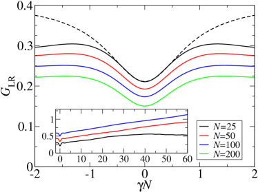
Figure 2: Average conductance for the three-kick model (17) as a function of the time-reversal symmetry breaking parameter $\gamma N$. Curves shown for $N=25,50,100$ and $200$ are offset vertically. The stochasticity parameter $K\approx 10$, $q=0.2$, and the dwell time $\tau_{\rm D}=5$. Inset: Same for a larger range of $\gamma N$ values.

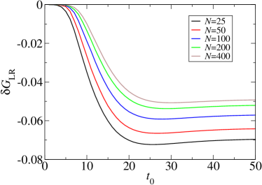
Figure 3: Time-resolved difference between ensemble-averaged conductance at $\gamma N=0$ and $\gamma N=0.7$ for the three-kick model (17). The dwell time is $\tau_{\rm D}=5$, while $K\approx 10$ and $q=0.2$

Figure 4: Left: Onset time $t_{\rm on}$ obtained from the time-resolved difference $G_{\rm LR}(\gamma)-G_{\rm LR}(0)$. Right: Weak localization correction $\delta G_{\rm LR}$, together with a fit $\propto\exp(-\tau_{\rm E}/\tau_{\rm D})$. The stochasticity parameter $K$ uniformly chosen between $10$ and $11.5$; the dwell times $\tau_{\rm D}$ is set at $\tau_{\rm D}=5$ and $\tau_{\rm D}=10$. For $\tau_{\rm D}=5$, data are shown for $\gamma N=0.7$ (circles), and $\gamma N=0.35$ (squares). For $\tau_{\rm D}=10$, data are shown for $\gamma N=0.3$ (diamonds) and $\gamma N=0.15$ (triangles).

Figure 5: Same as Figure 4, but for $K$ randomly chosen between $20$ and $23$.

Although our data are obtained in the same way as in Ref. Tworzydlo et al., 2004b, our conclusions are markedly different. Whereas Ref. Tworzydlo et al., 2004b finds no evidence of a systematic Ehrenfest-time dependence of weak localization, we conclude that there is a systematic Ehrenfest-time dependence of weak localization and that the simulation results for weak localization are consistent with the semiclassical theory. We attribute the differences to a lack of accuracy in the simulations of Ref. Tworzydlo et al., 2004b. Indeed, on average the simulations of Ref. Tworzydlo et al., 2004b do show a slight decrease upon increasing $N$, but the statistical uncertainties are too large to rule whether the decrease is systematic or accidental.

Figure 6 shows time-resolved data for $\delta G_{\rm LR}$ for $\tau_{\rm D}=12.8$, $q=0.3$, $\gamma N=0.2$, and $K$ taken uniformly in the interval $10<K<11.5$. Whereas the simulation data are consistent with the semiclassical theory for $N\gtrsim 20$ (see the insets in Fig. 6), the simulation results for $\delta G_{\rm LR}$ show significant deviations from the semiclassical theory for smaller channel numbers. This is no surprise, as the semiclassical theory is known to break down for small $N$. Despite the differences between the semiclassical theory and the magnitude of the simulated weak localization correction $\delta G_{\rm LR}$ for small $N$, the onset times appear to depend linearly on $\ln N$ down to the smallest channel numbers considered in the simulation ($N=5$).

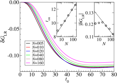
Figure 6: Time-resolved difference between ensemble-averaged conductance at $\gamma N=0$ and $\gamma N=0.2$ for the three-kick model (17), for $K\approx 10$ and $\tau_{\rm D}=12.8$. Left inset: onset times. Right inset: weak localization correction.

The second method of computing weak localization uses the scaling of the conductance with the number of channels, see Eq. (16). Time-resolved results for reflection and transmission coefficients are shown in Fig. 7 and 8, with $K$ taken randomly from the interval $10<K<11.5$ and dwell times $\tau_{\rm D}=5$ and $\tau_{\rm D}=10$, respectively. For $\tau_{\rm D}=5$, an average was taken over $80\,000$ samples, except for the data point at $N=400$. Due to the numerical cost of the calculations for $N=400$ only $40\,000$ samples were considered for $K\approx 10$ and $20\,000$ samples for $K\approx 20$. For $\tau_{\rm D}=10$, the average was taken over $20\,000$ samples for $K\approx 10$ and over $40\,000$ samples for $K\approx 20$. In all cases the statistical error of the weak localization correction was estimated to be $\sim 10^{-3}$. Again, we compare the data in Fig. 9 to lines with slopes which are fixed by the Lyapunov exponent of the corresponding classical map. For this model the Lyapunov exponents are $1.69$ when $K\approx 10$ and $2.37$ when $K\approx 20$. As for the three-kick model, the results are consistent with the semiclassical theory, see the right panel of Fig. 9. Figure 9 also contains results for $K$ taken uniformly in the interval $20<K<23$ (time-resolved data not shown).

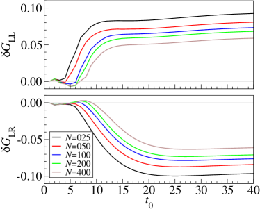
Figure 7: Weak localization correction to reflection and transmission coefficients, obtained using Eq. (16). Data shown are for $K\approx 10$ and $\tau_{\rm D}=5$. The average was taken over an ensemble of $80\,000$ realizations, except for $N=400$, as described in the text.

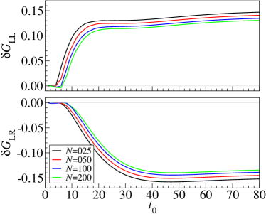
Figure 8: Weak localization correction to reflection and transmission coefficients, obtained using Eq. (16). Data shown are for $K\approx 10$ and $\tau_{\rm D}=10$. The number of realizations used to calculate the ensemble average is $20\,000$.

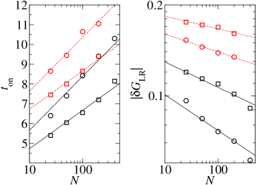
Figure 9: Left: Onset time $t_{\rm on}$ obtained from the time-resolved weak localization correction $\delta G_{\rm LR}$. Right: Weak localization correction $\delta G_{\rm LR}$, together with a fit $\propto\exp(-\tau_{\rm E}/\tau_{\rm D})$. Data are taken with stochasticity parameter $K$ uniformly chosen between $10$ and $11.5$ (circles) and between $20$ and $23$ (squares), and for dwell times $\tau_{\rm D}=5$ (solid) and $\tau_{\rm D}=10$ (dashed).

The time-resolved data shown in Figs. 7 and 8 show some structure at times smaller than the onset time. We cannot rule out that this structure, which appears to persist despite statistical averaging, affects our quantitative conclusions for the onset times and weak localization corrections. Since there is no such small-time structure in the weak localization data obtained by varying the field $\gamma$, we conclude that the small-time feature in the data of Figs. 7 and 8 must be a non-magnetic-field-dependent quantum correction (e.g., resulting from diffraction at the contacts). The feature disappears quickly upon increasing the stochasticity parameter $K$.

The largest channel numbers in our simulations — $N=200$ and $N=400$ for the scaling method, with an average over $80\,000$ and $40\,000$ samples (for $K\approx 10$), respectively — are smaller than the largest channel number used in the simulations Ref. Tworzydlo et al., 2004b. The observed decrease of the weak localization correction is statistically significant and systematic, but small. We could not obtain sufficiently accurate simulation data for higher number of channels. Increasing $N$ at fixed numerical cost implies that the number of realizations in the average has to scale $\propto N^{-2}$, so that the statistical error scales $\propto N$. Obtaining simulation data for $N=800$ at the same numerical cost as our $N=200$ data, would mean that only $5000$ samples can be averaged over, increasing the error by a factor $4$. At that point the statistical error becomes comparable to the expected incremental decrease of the weak localization data, and the simulation data loose statistical significance.

Shot noise. Figure 10 shows time-resolved data for the shot noise Fano factor $F$, taken for the one-kick model with stochasticity parameter $K\approx 10$ and dwell time $\tau_{\rm D}=5$. The statistical average was taken over $20$ realizations only, which is sufficient as the Fano factor is self-averaging for large channel numbers. A more quantitative analysis of the data for $K\approx 10$ (circles) , $K\approx 20$ (squares), $\tau_{\rm D}=5$ (solid lines), and $\tau_{\rm D}=10$ (dashed lines) is presented in the insets. Onset times, determined from the maximum of the $F(t_{0})$ graphs, are shown in the left inset of Fig. 10, together with a linear fit $\propto\tau_{\rm E}+\mbox{const}.$, using the Lyapunov exponents obtained from the corresponding classical map. The time of the maximum was defined as onset time since it is problematic to obtain reliable onset times using the definition used previously. However, numerically obtained onset times for shot noise are significantly impacted by the discreteness of the map’s time evolution, and do not show a smooth linear increase with $N$ over the range of channel numbers investigated in our simulations. The right inset of the figure shows values of the Fano factors for the limit of large truncation times, together with fits $\propto\exp(-\tau_{\rm E}/\tau_{\rm D})$, with the Lyapunov exponents $\lambda$ obtained from the corresponding classical map. We conclude that the rate of exponential suppression of shot noise upon increasing $N$ is consistent with the rate of exponential suppression of weak localization.

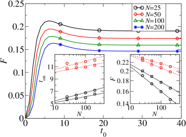
Figure 10: Time-resolved shot noise Fano factors for the open kicked rotator, with $K=10$ and $\tau_{\rm D}=5$. Left inset: Onset times, determined from the location of the maximum of time-resolved Fano factor as a function of the truncation time $t_{0}$. Right inset: Fano factor compared to a fit $\propto\exp(-\tau_{\rm E}/\tau_{\rm D})$. Results for $K\approx 10$ (circles), $K\approx 20$ (squares), $\tau_{\rm D}=5$ (solid lines), and $\tau_{\rm D}=10$ (dashed lines) are depicted in the insets.

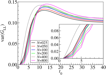
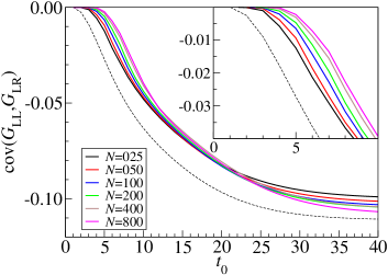
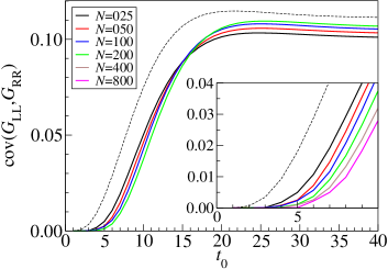
Figure 11: The truncation time-dependence of $\mbox{var}\,G_{\rm LL}$, $\mbox{cov}\,(G_{\rm LL},G_{\rm LR})$, and $\mbox{cov}\,(G_{\rm LL},G_{\rm RR})$ for the one-kick rotator. The dwell time is $\tau_{\rm D}=5$, while $K$ is chosen uniformly between $10$ and $11.5$. The corresponding time dependence given by random matrix theory is shown dashed. The short-time behavior is magnified in the inset.

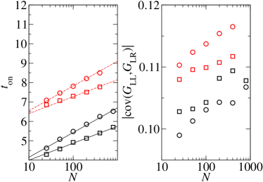
Figure 12: Left: Onset time $t_{\rm on}$ obtained from the time-resolved conductance covariance data. Right: Conductance covariance $\operatorname{cov}(G_{\rm LR},G_{\rm LL})$. Data are taken with stochasticity parameter $K$ uniformly chosen between $10$ and $11.5$ (squares) and between $20$ and $23$ (circles), and for dwell times $\tau_{\rm D}=5$ (solid) and $\tau_{\rm D}=10$ (dashed).

Conductance fluctuations. We performed time-resolved simulations for the variance of the reflection from the left contact $G_{\rm LL}$, the covariance of reflection $G_{\rm LL}$ and transmission $G_{\rm LR}$, and the covariance of reflections from the left and right contacts. We have computed the variance of the conductance coefficient $G_{\rm LL}$, as well as the covariances $\mbox{cov}\,(G_{\rm LL},G_{\rm LR})$ and $\mbox{cov}\,(G_{\rm LL},G_{\rm RR})$ as a function of the truncation time $t_{0}$. Unitarity of the scattering matrix implies that $\mbox{var}\,G_{\rm LL}=-\mbox{cov}\,(G_{\rm LL},G_{\rm LR})=\mbox{cov}\,(G_{\rm LL},G_{\rm RR})$ if $t_{0}\to\infty$, but this equality does not hold for finite $t_{0}$. Our simulations were done for dwell times $\tau_{\rm D}=5$ and $10$, and for stochasticity parameters $K$ between $10$ and $11.5$ and between $20$ and $23$. Results for $\tau_{\rm D}=5$ and $K\approx 10$, which are representative for all results obtained, are shown in Fig. 11. The number of realizations used for the averages shown here is $80\,000$ for $\tau_{\rm D}=5$, except for the $N=800$ data point, for which only $40\,000$ realizations were taken. The statistical error of the variances was estimated to be $\sim 10^{-4}$. Onset times calculated from the time-resolved covariance of $G_{\rm LL}$ and $G_{\rm LR}$ are shown in Fig. 12, together with conductance covariances. The scatter of the data points in the right panel of Fig. 12 for the short dwell time $\tau_{\rm D}=5$ is larger than our statistical error and reproducable. It is probably an artefact of the discrete time evolution of the map. (Note that similar scatter exists for the weak localization data, although, in that case, it is obscured by the large systematic decrease of the weak localization correction upon increasing $N$.)

As can be seen from the left panel of Fig. 12, the onset time depend linearly on $\ln N$: $\tau_{\rm on}\approx 0.55\ln N+\mbox{const}.$ for $K\approx 10$ and $\tau_{\rm on}\approx 0.38\ln N+\mbox{const.}$ for $K\approx 20$. However, the slopes are a factor $2.2$ smaller than for the weak localization data, both for $K\approx 10$ and $K\approx 20$. Further, the conductance variance (i.e., the large-$t_{0}$ limit of the data shown in Fig. 11) shows a slight increase with increasing $N$. The total increase is less than $10\%$ over the range of channel numbers considered in our simulations and falls within the statistical uncertainty of simulations reported in Refs. Jacquod and Sukhorukov, 2004; Tworzydlo et al., 2004c, a, where it was concluded that $\mbox{var}\,G$ is independent of $N$. Simulations of conductance fluctuations for the three-kick model slow a less than 10% decrease of $\mbox{var}\,G$ for the same range of $N$, as well as onset times that increase significantly slower with $N$ than the onset times for weak localization in the three-kick model (data not shown).

Clearly, the simulation data for conductance fluctuations are qualitatively different from the simulation data for weak localization; they differ both with respect to the $N$-dependence of the onset times and the $N$-dependence of the magnitude of the quantum corrections. This contradicts the notion that the same interference processes (diffusons and cooperons and their generalizations to ballistic systems) underly both weak localization and conductance fluctuations, although one should note that there is no semiclassical theory of the Ehrenfest-time dependence of conductance fluctuations yet.

III Quantum transport through chaotic cavities: semiclassical theory

A semiclassical theory for the Ehrenfest-time dependence of the weak localization correction in chaotic cavities was first formulated by Aleiner and Larkin.Aleiner and Larkin (1996) That theory predicts that the weak localization correction is suppressed $\propto\exp(-2\tau_{\rm E}/\tau_{\rm D})$. However, the analysis of Ref. Aleiner and Larkin, 1996 does not account for all classical correlations: it neglects the notion that no quantum diffraction takes place for electrons that spend less than a time $\tau_{\rm E}$ in the cavity. In this section we show that accounting for all classical correlations gives a weak localization correction that still depends exponentially on the Ehrenfest time, but with a different exponent: $\delta G\propto\exp(-\tau_{\rm E}/\tau_{\rm D})$. While a part of our calculations has already appeared elsewhere,Rahav and Brouwer (2005) this section includes a calculation of the full conductance matrix $G_{\alpha\beta}$. This allows to verify that unitarity is preserved. As the possible loss of unitarity is known to be a problem in semiclassical theories, it is important to demonstrate explicitly that the method used here preserves probability.

The system under consideration is a ballistic cavity with chaotic classical dynamics. The cavity is two-dimensional, and it is coupled to two electron reservoirs via contacts of width $d_{\rm L}$ and $d_{\rm R}$, see Fig. 13. Ergodicity of the electron motion inside the dot is ensured by the condition $d_{\rm L},d_{\rm R}\ll L$. The cavity and the contacts are considered in the semiclassical limit $d_{\rm L}k,d_{\rm R}k\gg 1$, where $k$ is the electron wavenumber.

Figure 13: Schematic picture of the ballistic chaotic cavity of size $L$. The cavity is attached to two leads, labeled “L” and “R”, and with width $d_{\rm L}$ and $d_{\rm R}$, respectively. The contours $C_{\rm L}^{\prime}$, $C_{\rm L}$, and $C_{\rm R}$ drawn in the leads are used for the calculation of transmission and reflection coefficients, see the text.

Thus, one has the separation of length scales $1/k\ll d_{\rm L},d_{\rm R}\ll L$ or, equivalently, the separation of time scales $(vk)^{-1}\ll\tau_{\rm erg}\ll\tau_{\rm D}$, where $v$ is the electron velocity, $\tau_{\rm erg}\sim L/v$ the ergodic time, and $\tau_{\rm D}$ the dwell time. The latter can be expressed as

$$\tau_{\rm D}^{-1}=\frac{(d_{\rm L}+d_{\rm R})v}{\pi{\cal A},}$$ (21)

where ${\cal A}$ is the area of the cavity. We also define

$$P_{\rm R}\equiv\frac{d_{\rm R}}{d_{\rm R}+d_{\rm L}},\ \ \ P_{\rm L}\equiv\frac{d_{\rm L}}{d_{\rm R}+d_{\rm L}}$$ (22)

as the probabilities that an electron at a random point in the cavity will leave through the right and left contacts, respectively. Electron motion inside the cavity is assumed to be fully phase coherent and electron-electron interactions are neglected.

The classical motion in the cavity is assumed to be fully chaotic (when closed), with a Lyapunov exponent $\lambda$. This exponent measures the rate of divergence of close phase space points. Since this divergence is due to scattering from the curved walls of the cavity one can expect that $\lambda\sim 1/\tau_{\rm erg}$. We neglect fluctuations in the Lyapunov exponent and assume that its value is uniform. This is done to simplify the calculation as much as possible and should not affect the main physical conclusions as long as relevant times are much longer than $\tau_{\rm erg}$.

The Aleiner-Larkin formalism is based on a semiclassical description of transport. Central objects in their theory are the non-oscillating parts of the product of an advanced and retarded Green functions. The “diffuson” is composed of combinations of orbits with themselves (known as the diagonal approximation in the semiclassical community) while the “cooperon” is composed of orbits and their time reversal counterparts. The equation of motion for the diffuson, neglecting quantum phenomena, is the Liouville equation,

$$\left[-i\omega+\hat{L}_{1}\right]{\cal D}^{0}(\omega;1,2)=\delta(1,2),$$ (23)

where $j\equiv(\phi_{j},{\bf R}_{j})=1,2$ denotes the phase space coordinates, limited to the energy shell: ${\bf R}$ is the electron position while the angle $\phi$ represents is the direction of the electron’s velocity $\mathbf{v}$. The operator $\hat{L}_{1}$ is the Liouville operator, taken with respect to the coordinates $(\phi_{1},\mathbf{R}_{1})$. For a hard wall cavity, $\hat{L}=\mathbf{v}\cdot{\partial}/{\partial\mathbf{R}}$, with appropriate boundary conditions at the walls. The symbol $\delta(1,2)$ denotes a delta function on the energy shell, that is, $\delta(1,2)\equiv 2\pi\delta({\bf R}_{1}-{\bf R}_{2})\delta(\phi_{1}-\phi_{2})$.

Quantum effects are introduced by including a weak additional random quantum potential, treating it as a perturbation, and averaging over its realizations.Aleiner and Larkin (1996) This random potential leads to two different effects, which are expected in a quantum theory. The first is a diffusion in phase space, which mimics the fact that quantum dynamics cannot separate small phase space structures. The second effect is ’quantum switching’ between close phase space trajectories, which results in weak localization. The strength $\gamma_{\rm q}$ of these effects is then set so that quantum corrections will appear after the correct time, the Ehrenfest time $\tau_{\rm E}$. Phase space diffusion modifies the evolution equation for the leading order diffuson asAleiner and Larkin (1996)

$$\left[-i\omega+\hat{L}_{1}-\gamma_{\rm q}\frac{\partial^{2}}{\partial\phi_{1}^{2}}\right]{\cal D}^{0}(\omega;1,2)=\delta(1,2).$$ (24)

the strength $\gamma_{\rm q}$ of the phase space diffusion term is estimated to be Aleiner and Larkin (1996) $\gamma_{\rm q}\simeq\lambda^{2}/kv$. It is instructive to note that this term, although small, breaks the time reversal invariance which is a property of both quantum mechanics and classical mechanics (in absence of a magnetic field). In the presence of quantum diffraction, the leading order cooperon, ${\cal C}^{0}$, also satisfies Eq. (24).

In addition to the presence of the phase space diffusion term in the evolution equation (24), quantum diffraction leads to an quantum correction to the diffuson: ${\cal D}={\cal D}^{0}+\Delta{\cal D}$. This quantum correction is referred to as weak localization, because similar quantum corrections are the precursor of Anderson localization in disordered systems. The weak localization correction for the diffuson readsAleiner and Larkin (1996)

$$\Delta{\cal D}(\omega;1,2)={\cal D}^{0}(\omega;1,\bar{2})\frac{{\cal C}^{0}(\omega;\bar{2},2)}{2\pi\hbar\nu}+\frac{{\cal C}^{0}(\omega;1,\bar{1})}{2\pi\hbar\nu}{\cal D}^{0}(\omega;\bar{1},2)\\ +\int d3{\cal D}^{0}(\omega;1,3){\cal D}^{0}(\omega;\bar{3},2)\left[2i\omega-\hat{L}_{3}+\gamma_{\rm q}\frac{\partial^{2}}{\partial\phi_{3}^{2}}\right]\frac{{\cal C}^{0}(\omega;3,\bar{3})}{2\pi\hbar\nu},$$ (25)

where $\bar{j}=(\phi_{j}+\pi,{\bf R}_{j})$ denotes the time reversal of phase space point $j$ and $\nu={m}/{2\pi\hbar^{2}}$ is the density of states per unit area. In terms of classical trajectories, the weak localization correction $\Delta{\cal D}$ corresponds to a configuration as shown in Fig. 1a: $\Delta{\cal D}$ is the correction to the product of a retarded and advanced Green function arising from the combination of a trajectory that intersects itself at a small angle and a trajectory that avoids intersecting itself.Aleiner and Larkin (1996); Sieber and Richter (2001) If the intersection angle is sufficiently small, such a pair of trajectories has strongly correlated actions, resulting in a net quantum correction to the diffuson even after ensemble averaging. The pairs of trajectories before and after the ‘interference region’ are represented by the leading-order diffusons ${\cal D}^{0}$ in Eq. (25), whereas the trajectories in the closed loop — an orbit conjugate to its time-reversed counterpart — are represented by the leading order cooperon ${\cal C}^{0}$.

In order to calculate the weak localization correction to the conductance, the dot’s conductance coefficients $G_{\rm LL}$ and $G_{\rm RL}$ are expressed in terms of the diffuson ${\cal D}$,

$$G_{\rm RL}=2\pi\hbar\nu v^{2}\int_{C_{\rm L}^{\prime}}dl_{1}\int_{\phi_{\rm L}^{\prime}-\pi/2}^{\phi_{\rm L}^{\prime}+\pi/2}\frac{d\phi_{1}}{2\pi}\cos(\phi_{\rm L}-\phi_{1})\int_{C_{\rm R}}dl_{2}\int_{\phi_{\rm R}-\pi/2}^{\phi_{\rm R}+\pi/2}\frac{d\phi_{2}}{2\pi}\cos(\phi_{{\rm R}}-\phi_{2}){\cal D}(2,1),$$ (26)

and

$$G_{\rm LL}=2\pi\hbar\nu v\int_{C_{\rm L}^{\prime}}dl_{1}\int_{\phi_{\rm L}^{\prime}-\pi/2}^{\phi_{\rm L}^{\prime}+\pi/2}\frac{d\phi_{1}}{2\pi}\cos(\phi_{{\rm L}}^{\prime}-\phi_{1})\left[v\int_{C_{\rm L}}dl_{2}\int_{\phi_{\rm L}-\pi/2}^{\phi_{\rm L}+\pi/2}\frac{d\phi_{2}}{2\pi}\cos(\phi_{\rm L}-\phi_{2}){\cal D}(2,1)-1\right].$$ (27)

Here $C_{\rm L}$, $C_{\rm R}$, and $C_{\rm L}^{\prime}$ are smooth contours following a cross section of the contacts, see Fig. 13. The contour $C_{\rm L}^{\prime}$ is taken a small amount further away from the cavity than the contour $C_{\rm L}$, see Fig. 13. The angles $\phi_{\rm L}$ and $\phi_{\rm R}$ denote the direction of the outward-pointing normal to $C_{\rm L}$, $C_{\rm R}$, whereas the angle $\phi_{\rm L}^{\prime}$ represents the direction of the inward-pointing normal to $C_{\rm L}^{\prime}$. Since we consider DC transport, the frequency $\omega$ has been set to zero. We refer to the Appendix for a derivation. Similar expressions, but with an ambiguity in the precise definitions of the integrals over the lead cross sections, were derived by Takane and Nakamura.Takane and Nakamura (1997)

The leading order “classical” transmission and reflection coefficients are found by substituting ${\cal D}^{0}$ for ${\cal D}$. Assuming that dynamics in the cavity is ergodic for all relevant time scales, one findsAleiner and Larkin (1996); Takane and Nakamura (1997)

$$G_{\rm RL}^{0}=-G_{\rm LL}^{0}=\frac{2\pi\hbar\nu{\cal A}}{\tau_{\rm D}}P^{\vphantom{2}}_{\rm L}P^{\vphantom{2}}_{\rm R},$$ (28)

where the escape probabilities to the left and right leads were defined in Eq. (22) above.

The weak localization correction to the conductance coefficients $G_{\rm RL}$ and $G_{\rm LL}$ is obtained by substituting Eq. (25), for the weak localization correction $\Delta{\cal D}$ of the diffuson, into Eqs. (26) and (27). We first consider the weak localization correction to $G_{\rm RL}$. The first two terms in (25) contain paths which leave the dot at the point of entry, and hence these do not contribute to the transmission. Hence

$$\delta G_{\rm RL}=-v^{2}\int_{C_{\rm L}^{\prime}}dl_{1}\int_{\phi_{\rm L}^{\prime}-\pi/2}^{\phi_{\rm L}^{\prime}+\pi/2}\frac{d\phi_{1}}{2\pi}\cos(\phi_{{\rm L}}^{\prime}-\phi_{1})\int_{C_{\rm R}}dl_{2}\int_{\phi_{\rm R}-\pi/2}^{\phi_{\rm R}+\pi/2}\frac{d\phi_{2}}{2\pi}\cos(\phi_{\rm R}-\phi_{2})\\ \times\int d3{\cal D}^{0}(2,3){\cal D}^{0}(\bar{3},1)\left[\hat{L}_{3}-\gamma_{\rm q}\frac{\partial^{2}}{\partial\phi_{3}^{2}}\right]{\cal C}^{0}(3,\bar{3}).$$ (29)

The phase space point 3 can be viewed as the center of the ’interference region’ as depicted in Fig. 1a. The two diffusons and the cooperon head into opposite directions in phase space, so that they will sample different parts of phase space along the trajectory. Thus, one can treat them as statistically uncorrelated.Aleiner and Larkin (1996)

Both the cooperon and the product of diffusons in Eq. (29) exhibit non-trivial correlations since the returning path is strongly correlated with the outgoing one, cf. Fig. 1a. In order to take into account these correlations one should examine what is meant by the phase space points $3$ and $\bar{3}$ in Eq. (29). By virtue of the phase-space diffusion term in the evolution equation for the leading order diffuson, effectively, the points $3$ and $\bar{3}$ do not need to be exactly time reversed phase space points, since quantum mechanics allows for a finite phase space uncertainty. An intuitive way to calculate the correlations between $3$ and $\bar{3}$ was shown by Vavilov and Larkin.Vavilov and Larkin (2003) Instead of using the diffusion in phase space, Vavilov and Larkin average over a range of initial phase space points near $3$ and final phase space points near $\bar{3}$. They show that the effect of the phase space diffusion is equivalent to such averaging (up to logarithmic corrections) if the ‘size’ of phase space area near $3$ and $\bar{3}$ scales as $k^{-1/2}$. [To be precise, the range of coordinates $\mathbf{R}$ in the average is $\sim(L/k)^{1/2}$, whereas the angular range is $\sim(Lk)^{-1/2}$.] We adopt the procedure of Vavilov and Larkin and consider an average over phase space points $3^{\prime}$ and $3^{\prime\prime}$ that are within a distance of order $k^{-1/2}$ of the phase space point $3$. We can then follow the classical orbits which start at the points $3^{\prime}$, $3^{\prime\prime}$. The phase space distance between these trajectories will diverge exponentially due to the chaotic dynamics. Since the trajectories start from phase space points at a distance $\sim k^{-1/2}$, it will take a time $\tau_{\rm E}/2$ to reach a phase space distance of order $L$. Once the phase space distance between the trajectories is large enough they can be considered as totally uncorrelated. At this point, ergodic dynamics can be assumed. The loss of correlations happens on a time scale of $1/\lambda$ around the time $\tau_{\rm E}/2$. Since $1/\lambda\ll\tau_{\rm E}$ in the parameter regime where the Ehrenfest time affects quantum transport, we can view this process as effectively instantaneous.

Let us first consider the cooperon in Eq. (29). As a result of the phase space correlations described above, one cannot close the orbit from $\bar{3}^{\prime}$ to $3^{\prime\prime}$ for short times. In order to make this more quantitative, we denote by $t_{j}$ the time it takes for the classical orbit starting at phase space point $j$ to leave the cavity through one of the two openings. Then, if $t_{\bar{3}}<\tau_{\rm E}/2$ we find ${\cal C}^{0}(3,\bar{3})={\cal C}^{0}(3^{\prime\prime},\bar{3}^{\prime})=0$. On the other hand, if $t_{\bar{3}}>\tau_{\rm E}/2$ we can propagate the phase space point $\bar{3^{\prime}}$ for a time $\tau_{\rm E}/2$ and reach phase space point $4$. Similarly, we can propagate $3^{\prime\prime}$ backward in time and find, toward the phase space point $5$. This leads to

$${\cal C}^{0}(3^{\prime\prime},\bar{3^{\prime}})\simeq\left\{\begin{array}[]{ll}0&\mbox{if $t_{\bar{3}}<{\tau_{\rm E}}/{2}$},\\ {\cal C}^{0}(5,4)&\mbox{if $t_{\bar{3}}>{\tau_{\rm E}}/{2}$}.\end{array}\right.$$

When the phase space points $3^{\prime}$ and $3^{\prime\prime}$ are averaged over, the cooperon will have contributions from various phase space points $5,4$, which are their distant past (or future). The points $4$ and $5$ can be taken to be uncorrelated and sample the phase space with uniform probability. Since the phase space point $3$ is eventually integrated over, there will be contributions from a sizable fraction of phase space. Thus, we approximate the average contribution to the cooperon by replacing ${\cal C}^{0}(5,4)$ by its average value $\tau_{\rm D}/{\cal A}$. This leads to

$$\left<{\cal C}^{0}(3,\bar{3})\right>=\frac{\tau_{\rm D}}{\cal A}\theta(t_{\bar{3}}-\tau_{\rm E}/2),$$ (30)

where $\theta(x)=1$ if $x>0$ and $0$ otherwise.

We address the product of two diffusons in Eq. (29) by considering the integral

$${\cal I}(3)=-v^{2}\int_{C_{\rm L}^{\prime}}dl_{1}\int_{\phi_{\rm L}^{\prime}-\pi/2}^{\phi_{\rm L}^{\prime}+\pi/2}\frac{d\phi_{1}}{2\pi}\cos(\phi_{\rm L}^{\prime}-\phi_{1})\\ \times\int_{C_{\rm R}}dl_{2}\int_{\phi_{\rm R}-\pi/2}^{\phi_{\rm R}+\pi/2}\frac{d\phi_{2}}{2\pi}\cos(\phi-\phi_{2}){\cal D}^{0}(2,3){\cal D}^{0}(\bar{3},1).$$ (31)

Again, the integration over phase space points $3$ and $\bar{3}$ is replaced by an average over phase space points $3^{\prime}$ and $3^{\prime\prime}$ within a distance of order $(L/k)^{1/2}$ from 3. Since the diffuson connects the phase space points $3^{\prime}$ and $3^{\prime\prime}$ with points at two different contacts, the product of diffusons must be zero if $t_{3}<\tau_{\rm E}/2$ where, as before, $t_{3}$ is the time it takes for the orbit at phase space point $3$ to leave the system. For larger $t_{3}$ we may, again, assume ergodicity, so that we find, after averaging over $3^{\prime}$ and $3^{\prime\prime}$,

$${\cal I}(3)=P_{\rm R}P_{\rm L}\theta(t_{3}-\tau_{\rm E}/2).$$

Combining results, we find

$$\delta G_{\rm RL}=-P_{\rm R}P_{\rm L}\frac{\tau_{\rm D}}{\cal A}\int d3\theta(t_{3}-\tau_{\rm E}/2)\hat{L}_{3}\theta(t_{\bar{3}}-\tau_{\rm E}/2).$$ (32)

The Liouville operator in Eq. (32) measures the rate of flow of probability density out of the integration range of the phase space variable $3$.Aleiner and Larkin (1996) The boundary of the integration range is composed of the lead phase space points propagated backward for a time $t_{\rm E}/2$. This leaves only a fraction $\exp({-\frac{\tau_{\rm E}}{2\tau_{\rm D}}})$ of the size of the boundary at the lead. To estimate the integral we assume that each outgoing direction is equally likely to be in the system when propagated backward. However, only points which also have $t_{\bar{3}}>\tau_{\rm E}/2$ will have a non-vanishing cooperon, leading to an additional factor of $\exp({-\frac{\tau_{\rm E}}{2\tau_{\rm D}}})$. Collecting contributions from both leads, we find

$$\delta G_{\rm RL}=-P_{\rm R}P_{\rm L}e^{-\tau_{\rm E}/\tau_{\rm D}}.$$ (33)

It is of interest to compute also the weak localization correction $\delta G_{\rm LL}$. This will allow to check that probability is conserved. The calculation is similar to that of the $\delta G_{\rm RL}$, with two important differences. The first difference is that the weak localization correction of reflection is composed from two parts. In addition to the third term in Eq. (25), there is a contribution from the second term in Eq. (25). We write these two parts as $\delta G_{{\rm LL}}^{(1)}$ and $\delta G_{\rm LL}^{(2)}$, respectively, and calculate them separately. Substitution of the third term in Eq. (25) into Eq. (27) gives

$$\delta G_{\rm LL}^{(1)}=-v^{2}\int_{C_{\rm L}^{\prime}}dl_{1}\int_{\phi_{\rm L}^{\prime}-\pi/2}^{\phi_{\rm L}^{\prime}+\pi/2}\frac{d\phi_{1}}{2\pi}\cos(\phi_{\rm L}^{\prime}-\phi_{1})\int_{C_{\rm L}}dl_{2}\int_{\phi_{\rm L}-\pi/2}^{\phi_{\rm L}+\pi/2}\frac{d\phi_{2}}{2\pi}\cos(\phi_{{\rm L}}-\phi_{2})\\ \times\int d3{\cal D}^{0}(2,3){\cal D}^{0}(\bar{3},1)\left[\hat{L}_{3}-\frac{1}{\tau_{q}}\frac{\partial^{2}}{\partial\phi_{3}^{2}}\right]{\cal C}^{0}(3,\bar{3}).$$ (34)

The product of the two diffusons can be assumed to be uncorrelated with the cooperon. The calculation of the cooperon proceeds as for the transmission calculation. However, the behavior of the product of the diffusons contributing to reflection differ from that of the diffusons contributing to transmission. To see that, again consider the integral

$${\cal I}(3)=-v^{2}\int_{C_{\rm L}^{\prime}}dl_{1}\int_{\phi_{\rm L}^{\prime}-\pi/2}^{\phi_{\rm L}^{\prime}+\pi/2}\frac{d\phi_{1}}{2\pi}\cos(\phi_{\rm L}^{\prime}-\phi_{1})\int_{C_{\rm L}}dl_{2}\int_{\phi_{\rm L}-\pi/2}^{\phi_{\rm L}+\pi/2}\frac{d\phi_{2}}{2\pi}\cos(\phi_{{\rm L}}-\phi_{2}){\cal D}^{0}(2,3){\cal D}^{0}(\bar{3},1).$$

If $t_{3}>\tau_{\rm E}/2$ both diffusons become uncorrelated before leaving the system and the average value of this integral is therefore $P_{\rm L}^{2}$. However, if $t_{3}<\tau_{\rm E}/2$ both diffusons will exit the dot through the same lead, and one finds ${\cal I}=P_{\rm L}$. Hence,

$${\cal I}=\left\{\begin{array}[]{ll}P_{\rm L}&\mbox{if $t_{\bar{3}}<{\tau_{\rm E}}/{2}$};\\ P_{\rm L}^{2}&\mbox{if $t_{\bar{3}}>{\tau_{\rm E}}/{2}$}.\end{array}\right.$$

This is the second difference between the calculations of $\delta G_{\rm RL}$ and $\delta G_{\rm LL}$. We then find

$$\delta G_{\rm LL}^{(1)}=-P_{\rm L}e^{-\tau_{\rm E}/2\tau_{\rm D}}(1-e^{-\tau_{\rm E}/2\tau_{\rm D}})-P_{\rm L}^{2}e^{-\tau_{\rm E}/\tau_{\rm D}}.$$ (35)

The contribution $\delta G_{\rm LL}^{(2)}$ is obtained by substituting the second term in the right hand side of Eq. (25) into Eq. (27). The lead integral over $2$ can be calculated, resulting in

$$\delta G_{\rm LL}^{(2)} = v\int_{C_{\rm L}}dl_{1}\int_{\phi_{\rm L}-\pi/2}^{\phi_{\rm L}+\pi/2}\frac{d\phi_{1}}{2\pi}\cos(\phi_{\rm L}-\phi_{1}){\cal C}^{0}(1,\bar{1})$$ (36)

$$= P_{\rm L}e^{-\tau_{\rm E}/2\tau_{\rm D}}.$$

Combining Eqs. (36) and (35), one finds $\delta G_{\rm LL}=\delta G_{\rm LL}^{(1)}+\delta G_{\rm LL}^{(2)}=-\delta G_{\rm RL}$, as expected.

The result (33) shows that, according to the semiclassical theory, the weak localization correction to transmission is suppressed exponentially. However, the exponent we find is different from that of Ref. Aleiner and Larkin, 1996, where it is reported that $\delta G_{\rm RL}=-P_{\rm L}P_{\rm R}\exp(-2\tau_{\rm E}/\tau_{\rm D})$. The reason for the difference with Ref. Aleiner and Larkin, 1996 is that our calculation obeys the classical correlations following from the separation of phase space into a ‘classical’ and ‘quantum’ part, corresponding to (classical) trajectories of length smaller or larger than $\tau_{\rm E}$, respectively. Quantum diffraction does not involve the ‘classical’ part of phase space. Calculating the cooperon and the product of diffuson propagators assuming ergodic dynamics in the ‘quantum’ part of phase space only increases the weak localization correction $\delta G$ by a factor $\exp(\tau_{\rm E}/\tau_{\rm D})$ with respect to the calculation of Ref. Aleiner and Larkin, 1996. The reason that $\delta G$ remains exponentially small — but with exponent $\exp(-\tau_{\rm E}/\tau_{\rm D})$, not $\exp(-2\tau_{\rm E}/\tau_{\rm D})$ — is that, according to the semiclassical theory, weak localization requires a minimal path length of $2\tau_{\rm E}v$. The fraction of ‘quantum’ trajectories that remain inside the cavity during the time period $2\tau_{\rm E}$ is exponentially small, $\propto\exp(-\tau_{\rm E}/\tau_{\rm D})$, hence the exponentially small weak localization correction if $\tau_{\rm E}\gg\tau_{\rm D}$.

Sofar we have considered the weak localization correction to the transmission. What about other quantum interference effects, such as the transmission fluctuations? Takane and Nakamura have extended the semiclassical theory of Aleiner and Larkin to the conductance variance $\mbox{var}\,G$, but for the limit $\tau_{\rm E}\to 0$ only.Takane and Nakamura (1998) They found $\mbox{var}\,G=2(P_{\rm L}P_{\rm R})^{2}$, in agreement with predictions from random matrix theory.Beenakker (1997) Just as the semiclassical theory for the weak localization correction $\delta G_{\rm RL}$ was simpler than the semiclassical theory for $\delta G_{\rm LL}$ (see above), the semiclassical theory of transmission fluctuations takes its simplest form if applied to the covariance of reflection from the right contact $G_{\rm RR}$ and reflection from the left contact $G_{\rm LL}$. Of course, unitarity implies $\mbox{var}\,G=\mbox{cov}\,(G_{\rm LL},G_{\rm RR})$. In Ref. Takane and Nakamura, 1998, only one contribution to the conductance covariance $\mbox{cov}\,(G_{\rm LL},G_{\rm RR})$ was considered. This contribution corresponds to the four trajectories shown in Fig. 1b. For these four trajectories, a minimal dwell time $2\tau_{\rm E}$ is required: classical trajectories originating from each of the openings need to diverge and reunite, each of which takes a time $\tau_{\rm E}$. Hence, following the same phase space arguments as for the weak localization correction, we anticipate that their contribution to the conductance fluctuations depends on the Ehrenfest times as

$$[\mbox{cov}\,(G_{\rm LL},G_{\rm RR})]^{1/2} = [\mbox{var}\,G]^{1/2}\propto e^{-\tau_{\rm E}/\tau_{\rm D}}$$ (37)

$$\ \ \mbox{if $\tau_{\rm E}\gg\tau_{\rm D}$}.$$

However, there may be contributions to the conductance fluctuations other than that of Fig. 1b. (This possibility can not be excluded on the basis of Ref. Takane and Nakamura, 1998.) For example, there may be trajectories that involve small-angle intersections of three trajectories at the same point.Tian and Larkin (2004); Müller et al. (2004) While it is not expected that the inclusion of such trajectories undo the suppression of the conductance fluctuations in the limit $\tau_{\rm E}\gg\tau_{\rm D}$, they may have a non-negligible contribution for $\tau_{\rm E}\sim\tau_{\rm D}$.

A final note about the results presented in this section: In the calculation performed in this section we have replaced dynamical functions by their averages. For example, the probability that a wave packet will exit through a given lead is (almost) $1$ or $0$ for short enough times, depending on the classical dynamics, not $P_{\rm L}$ or $P_{\rm R}$. Thus, we have actually estimated the ensemble average of the weak localization correction. One can expect that if a system is close to the classical limit there will be more fluctuations in the values of diffusons and cooperons. This may lead to large deviations of the weak localization correction from that of systems with small Ehrenfest times, and to large classical conductance fluctuations.Tworzydlo et al. (2004c) In order to describe these fluctuations quantitatively, one needs a sample-specific theory for the dynamics of the diffuson, which covers the times of order $\tau_{\rm E}$ exactly. While this is an important theoretical problem, it is beyond the scope of this paper, and should not affect the eventual exponential suppression of quantum interference phenomena for large Ehrenfest times.

IV Discussion

In Sec. II, we reported results of numerical simulations for weak localization, conductance fluctuations, and shot noise of the open quantum kicked rotator. The numerical simulations for weak localization and shot noise are consistent with an exponential suppression $\propto\exp(-\tau_{\rm E}/\tau_{\rm D})$, in quantitative agreement with the semiclassical theory of Sec. III. The numerical simulations for conductance fluctuations show a small increase with increasing Ehrenfest time, not inconsistent with previous simulation data reported in the literature.Jacquod and Sukhorukov (2004); Tworzydlo et al. (2004c, a) Our simulations also give information on the minimal time at which quantum effects occur. For weak localization and shot noise, these times are $2\tau_{\rm E}$ and $\tau_{\rm E}$, respectively, consistent with semiclassical theory. For conductance fluctuations, the onset time is less than half the onset time of weak localization. (Note that it is possible that some contribution for weak localization in reflection may appear after a time of $\tau_{\rm E}$.)

In order to explain the numerical simulations of shot noise, weak localization, and universal conductance fluctuations, the authors of Refs. Tworzydlo et al., 2003; Jacquod and Sukhorukov, 2004; Tworzydlo et al., 2004c, a proposed a phenomenological alternative to the standard semiclassical theory, referred to as ‘effective random matrix theory’. Guiding principle for the effective random matrix theory is that quantum diffraction takes place between trajectories with dwell times larger than $\tau_{\rm E}$ only; trajectories with dwell time shorter than $\tau_{\rm E}$ build scattering states with transmission (exponentially close to) $0$ or $1$ and do not contribute to shot noise, weak localization, or universal conductance fluctuations. The importance of ‘quantum’ trajectories is described by an effective number of ‘quantum channels’ $N_{\rm q}\sim N\exp(-\tau_{\rm E}/\tau_{\rm D})$. Following Silvestrov et al.,Silvestrov et al. (2003) it was then proposed that the scattering of ‘quantum channels’ is described by random matrix theory as long as $N_{\rm q}\gg 1$. The condition $N_{\rm q}\gg 1$ is generically met, even if $\tau_{\rm E}\gg\tau_{\rm D}$.

The effective random matrix theory not only correctly predicts the suppression of the ensemble-averaged shot noise at large Ehrenfest times — shot noise is proportional to the number of channels $N$, which is replaced by $N_{\rm q}=N\exp(-\tau_{\rm E}/\tau_{\rm D})$ in the effective random matrix theory —, it also describes sample-specific deviations from the ensemble average that arise from the classical dynamics.Tworzydlo et al. (2003) The effective random matrix also has had remarkable success explaining other observables that are proportional to the channel number $N$, such as the density of transmission eigenvalues,Jacquod and Whitney (2005) as well as the density of states in a chaotic cavity coupled to a superconductor.Silvestrov et al. (2003) On the other hand, quantum-interference effects, such as weak localization and conductance fluctuations are independent of $N$, and, hence, are predicted to be independent of the Ehrenfest time. Thus, for weak localization, the effective random matrix theory differs from the semiclassical theory, which predicts a suppression $\propto\exp(-\tau_{\rm E}/\tau_{\rm D})$.

The effective random matrix theory and the semiclassical description of transport not only disagree regarding the magnitude of the weak localization correction to the conductance, they also disagree with regard to the minimal time required for quantum interference effects to occur. In the semiclassical theory, quantum interference requires a minimal wavepacket to be split and reunited, which takes a minimal time $2\tau_{\rm E}$. This is in contrast to the effective random matrix theory, where quantum interference is fully established already after a time $\tau_{\rm E}$. Interestingly, there is no difference between semiclassics and effective random matrix theory for shot noise: Not being a quantum interference effect, shot noise only requires wavepackets to be split, which happens after a time $\tau_{\rm E}$ in both theories.

These two differences between the semiclassical theory for weak localization and the effective random matrix theory are not unrelated. Both theories are consistent with a fully classical description of electron dynamics for the first time interval of length $\tau_{\rm E}$ after the electron has entered the cavity. Differences between the two theories appear for electrons that escape from the cavity in the second time interval of length $\tau_{\rm E}$ (i.e., for times between $\tau_{\rm E}$ and $2\tau_{\rm E}$). In the semiclassical theory, electrons that escape during this interval behave quantum mechanically but do not contribute to weak localization. As explained in Sec. III, the escape of electrons between $\tau_{\rm E}$ and $2\tau_{\rm E}$ is responsible for the suppression of weak localization with exponent $\exp(-\tau_{\rm E}/\tau_{\rm D})$ in the semiclassical theory. In the effective random matrix theory, weak localization sets in as soon as the classical description fails, one Ehrenfest time after the electron enters the cavity; there is no time interval in which electron dynamics is neither fully classical nor described by random matrix theory.

A ‘microscopic theory’ supporting the effective random matrix theory and its prediction of Ehrenfest-time independent weak localization and conductance fluctuations appeared recently.Whitney and Jacquod (2005) This theory is based on the assumption that electron dynamics in the quantum trajectories (i.e., trajectories with dwell times larger than $\tau_{\rm E}$) is fully ergodic, with fully established quantum interference corrections. Such an assumption violates the semiclassical picture of weak localization, in which the quantum correction only appears after a time $2\tau_{\rm E}$. Hence, a theory which tries to justify the effective random matrix theory must provide an entirely new semiclassical model for weak localization, in which the quantum correction appears after one Ehrenfest time only.

Although, at present, there is no theory that explains all simulation data, we can conclude that our time-resolved simulation data for the quantum interference corrections to the conductance are not consistent with the effective random matrix theory. First, because the effective random matrix theory predicts onset time $\tau_{\rm E}$ for weak localization, as well as an Ehrenfest-time independent weak localization correction, both of which are ruled out by our simulations. Second, because simulation results for weak localization and conductance fluctuations are qualitatively different, whereas the ‘effective random matrix theory’ predicts equal onset times and Ehrenfest-time dependences for weak localization and conductance fluctuations.

Of course, the question why numerical simulations for weak localization and conductance fluctuations in the open quantum kicked rotator are qualitatively different remains. Clearly, this question can not receive a final answer as long as there is no semiclassical theory for the Ehrenfest-time dependence of conductance fluctuations. Given the difficulty of obtaining accurate numerical results in the regime $\tau_{\rm E}\gg\tau_{\rm D}$, such a semiclassical theory needs to include the parameter range $\tau_{\rm E}\sim\tau_{\rm D}$ if a valid comparison with the numerical simulations is to be made.

Appendix A Transmission and reflection in terms of diffusons

In this Appendix the transmission and reflection through a quantum dot are derived in terms of lead integrals of a diffuson. Similar expressions were derived previously by Takane and Nakamura.Takane and Nakamura (1997) However, their expressions are ambiguous with respect to the exact locations of the cross sections in the leads. In our approach, all ambiguities are resolved.

To calculate the total transmission and reflection in terms of diffusons, it is useful to obtain expressions for scattering matrix elements using the retarded Green function of the cavity. Exact expressions of this type were derived in Refs. Stone and Szafer, 1988; Baranger and Stone, 1989. The leads have a uniform cross section, so that the lead wavefunction can be decomposed into free waves along the lead (denoted by $x$ coordinates) and a basis of transverse wavefunctions $\chi_{a}(y)$. The same decomposition can also be used for the retarded Green function (at the Fermi energy), and one defines

$${\cal G}^{+}({\bf r}_{1},{\bf r}_{2})=\sum_{mn}{\cal G}^{+}_{mn}(x_{1},x_{2})\chi_{m}(y_{1})\chi^{*}_{n}(y_{2}),$$ (38)

for coordinates ${\bf r}_{1}$ and ${\bf r}_{2}$ in the leads. We use the convention that different leads are assigned different modes, so that Eq. (38) remains meaningful if ${\bf r}_{1}$ and ${\bf r}_{2}$ are in different leads.

Using the asymptotics of ${\cal G}^{+}$ and of the scattering states, the Green function in the leads can be written in terms of scattering matrix elements $S_{mn}$. One findsStone and Szafer (1988)

$${\cal G}^{+}_{mn}(x_{1},x_{2})=-\frac{i}{v_{n}}\left[\delta_{mn}e^{ik_{n}(x_{1}-x_{2})}\rule{0.0pt}{17.0pt}\right.\\ +\left.S_{mn}\sqrt{\frac{k_{n}}{k_{m}}}e^{-ik_{n}x_{2}-ik_{m}x_{1}}\rule{0.0pt}{17.0pt}\right],$$ (39)

for $x_{1}>x_{2}$ with $x_{1,2}$ in the left lead, and to

$${\cal G}^{+}_{mn}(x_{1},x_{2})=-\frac{i}{v_{n}}S_{mn}\sqrt{\frac{k_{n}}{k_{m}}}e^{ik_{m}x_{1}-ik_{n}x_{2}},$$ (40)

for $x_{1}$ in the right lead while $x_{2}$ is in the left lead. (In the following we use units where $\hbar=1$.) For the following discussion it is important to emphasize the condition $x_{1}>x_{2}$, which appears when both $x_{1}$ and $x_{2}$ are in the same lead. One of the steps in the derivation of Eq. (39) involves an integral over a finite domain (bounded by the cross-section $x=x_{2}$), where the integrand is proportional to $\delta({\bf r}_{1}-{\bf r}_{2})$. This integral will give different results depending whether ${\bf r}_{1}$ is in the domain of integration ($x_{1}>x_{2}$) or not ($x_{1}<x_{2}$). This leads to the inequality in Eq. (39). Later, when we write ${\cal G}^{+}_{mn}$ in terms of cross section integrals, two different cross sections, at $x_{1}$ and $x_{2}$, are obtained.

To compute the conductance coefficients $G_{\rm LL}$ and $G_{\rm LR}$, the absolute value squared of the matrix elements is needed. It can be expressed in terms of Green function with the help of

$$\left(\frac{\partial}{\partial x_{1}}-\frac{\partial}{\partial x_{4}}\right)\left(\frac{\partial}{\partial x_{2}}-\frac{\partial}{\partial x_{3}}\right)\\ \times{\cal G}^{+}_{mn}(x_{1},x_{2})\left.\left[{\cal G}^{+}_{mn}(x_{4},x_{3})\right]^{*}\right|_{\begin{subarray}{l}x_{1}=x_{4}\\ x_{2}=x_{3}\end{subarray}}=\\ \left\{\begin{array}[]{ll}4m^{2}|S_{mn}|^{2}&\mbox{ if }x_{1}\in R,x_{2}\in L\\ 4m^{2}\left(\delta_{mn}-|S_{mn}|^{2}\right)&\mbox{ if }x_{1},x_{2}\in L,x_{1}>x_{2}.\end{array}\right.$$ (41)

The conductance coefficients $G_{\rm LL}$ and $G_{\rm LR}$ are then calculated using Eq. (II). One can use Eq. (41) to simplify the summations, since the lead modes enter into ${\cal G}_{mn}^{+}$ via cross section integrals over the leads. One then uses

$$\sum_{n=1}^{N}\chi_{n}^{*}(y_{1})\chi_{n}(y_{4})\simeq\delta_{\lambda_{F}}(y_{1}-y_{4}).$$ (42)

Replacing this approximate finite width delta function by an exact one leads, after a straightforward calculation, to

$$G_{\rm RL} =\frac{1}{4m^{2}}\int_{C_{\rm R}}dy_{1}\int_{C_{\rm L}^{\prime}}dy_{2}\left(\frac{\partial}{\partial x_{1}}-\frac{\partial}{\partial x_{4}}\right)$$

$$\times\left(\frac{\partial}{\partial x_{2}}-\frac{\partial}{\partial x_{3}}\right)\left.{\cal G}^{+}({\bf r}_{1},{\bf r}_{2})\left[{\cal G}^{+}({\bf r}_{4},{\bf r}_{3})\right]^{*}\right|_{\begin{subarray}{l}{\bf r}_{1}={\bf r}_{4}\\ {\bf r}_{2}={\bf r}_{3}\end{subarray}}$$ (43)

$$G_{\rm LL} =-\frac{1}{4m^{2}}\int_{C_{\rm L}}dy_{1}\int_{C_{\rm L}^{\prime}}dy_{2}\left(\frac{\partial}{\partial x_{1}}-\frac{\partial}{\partial x_{4}}\right)$$

$$\times\left(\frac{\partial}{\partial x_{2}}-\frac{\partial}{\partial x_{3}}\right)\left.{\cal G}^{+}({\bf r}_{1},{\bf r}_{2})\left[{\cal G}^{+}({\bf r}_{4},{\bf r}_{3})\right]^{*}\right|_{\begin{subarray}{l}{\bf r}_{1}={\bf r}_{4}\\ {\bf r}_{2}={\bf r}_{3}\end{subarray}}.$$ (44)

This expressions differ from those in Ref. Takane and Nakamura, 1997 in that the integrals for the reflection are along separate cross sections, with the cross section $C_{\rm L}$ closer to the cavity than $C_{\rm L}^{\prime}$.

On each of the cross sections there are two points which are almost identified: ${\bf r}_{1}\simeq{\bf r}_{4}$ and ${\bf r}_{2}\simeq{\bf r}_{3}$. Therefore, it is natural the use the following Fourier transform Aleiner and Larkin (1996); Takane and Nakamura (1997)

$${\cal G}^{+}({\bf r}_{1},{\bf r}_{2}){\cal G}^{-}({\bf r}_{3},{\bf r}_{4})=\int\frac{d{\bf p}_{1}}{(2\pi)^{2}}\int\frac{d{\bf p}_{2}}{(2\pi)^{2}}e^{i{\bf p}_{1}\cdot({\bf r}_{1}-{\bf r_{4}})}\\ \times e^{i{\bf p}_{2}\cdot({\bf r}_{3}-{\bf r_{2}})}K^{\cal D}({\bf p}_{1},{\bf R}_{1};{\bf p}_{2},{\bf R}_{2}),$$ (45)

where ${\bf R}_{1}=({\bf r}_{1}+{\bf r}_{4})/2$ and ${\bf R}_{2}=({\bf r}_{2}+{\bf r}_{3})/2$. Note that ${\bf R}_{1}$ and ${\bf R}_{2}$ are on the cross sections of the lead. Energy conservation can be used to simplify this probability density further. This is done by defining

$$K^{\cal D}({\bf p}_{1},{\bf R}_{1};{\bf p}_{2},{\bf R}_{2})=\frac{2\pi}{\nu}\delta\left(E_{F}-\frac{p_{1}^{2}}{2m}\right)\delta\left(E_{F}-\frac{p_{2}^{2}}{2m}\right)\\ \times{\cal D}({\bf n}_{1},{\bf R}_{1};{\bf n}_{2},{\bf R}_{2}).$$ (46)

Substitution of (45) and (46) in (A) will lead to the expressions for $G_{\rm RL}$ and $G_{\rm LL}$ in terms of the diffuson. The calculation is straightforward. Some care is needed only when one determines the boundary conditions. For $G_{\rm RL}$, only diffusions that go into the cavity can get from the left lead into the right lead. These diffusons can arrive to the right lead only if they originate from the cavity. These considerations result in the Theta functions in Eq. (26). The calculation for $G_{\rm LL}$ is very similar. The only difference is that both incoming and outgoing diffusons will cross the inner ($C_{\rm L}$) cross section. However, all the incoming probability flux from $C_{\rm L}^{\prime}$ must cross $C_{\rm L}$. This incoming flux just cancels the $N_{\rm L}$ factor in (44). The remaining contribution results in Eq. (27).

References

- Zaslavsky (1981) G. M. Zaslavsky, Phys. Rep. 80, 157 (1981).
- Aleiner and Larkin (1996) I. L. Aleiner and A. I. Larkin, Phys. Rev. B 54, 14423 (1996).
- Beenakker and van Houten (1991a) C. W. J. Beenakker and H. van Houten, Solid State Physics 44, 1 (1991a).
- Beenakker (1997) C. W. J. Beenakker, Rev. Mod. Phys. 69, 731 (1997).
- Beenakker and van Houten (1991b) C. W. J. Beenakker and H. van Houten, Phys. Rev. B 43, 12066 (1991b).
- Agam et al. (2000) O. Agam, I. Aleiner, and A. Larkin, Phys. Rev. Lett. 85, 3153 (2000).
- Oberholzer et al. (2002) S. Oberholzer, E. V. Sukhorukov, and C. Schönenberger, Nature 415, 765 (2002).
- Tworzydlo et al. (2003) J. Tworzydlo, A. Tajic, H. Schomerus, and C. W. J. Beenakker, Phys. Rev. B 68, 115313 (2003).
- Jacquod and Sukhorukov (2004) P. Jacquod and E. V. Sukhorukov, Phys. Rev. Lett. 92, 116801 (2004).
- Jacquod and Whitney (2005) P. Jacquod and R. S. Whitney, cond-mat/0506440 (2005).
- Rahav and Brouwer (2005) S. Rahav and P. W. Brouwer, Phys. Rev. Lett. 95, 056806 (2005).
- Adagideli (2003) I. Adagideli, Phys. Rev. B 68, 233308 (2003).
- Yevtushenko et al. (2000) O. Yevtushenko, G. Lütjering, D. Weiss, and K. Richter, Phys. Rev. Lett. 84, 542 (2000).
- Argaman (1995) N. Argaman, Phys. Rev. Lett. 75, 2750 (1995).
- Argaman (1996) N. Argaman, Phys. Rev. B 53, 7035 (1996).
- Takane and Nakamura (1997) Y. Takane and K. Nakamura, J. Phys. Soc. Japan 66, 2977 (1997).
- Takane and Nakamura (1998) Y. Takane and K. Nakamura, J. Phys. Soc. Japan 67, 397 (1998).
- Tworzydlo et al. (2004a) J. Tworzydlo, A. Tajic, H. Schomerus, P. W. Brouwer, and C. W. J. Beenakker, Phys. Rev. Lett. 93, 186806 (2004a).
- Jacquod et al. (2003) P. Jacquod, H. Schomerus, and C. W. J. Beenakker, Phys. Rev. Lett. 90, 207004 (2003).
- Stöckmann (1999) H. J. Stöckmann, Quantum Chaos: An Introduction (Cambridge University Press, 1999).
- Tworzydlo et al. (2004b) J. Tworzydlo, A. Tajic, and C. W. J. Beenakker, Phys. Rev. B 70, 205324 (2004b).
- Tworzydlo et al. (2004c) J. Tworzydlo, A. Tajic, and C. W. J. Beenakker, Phys. Rev. B 69, 165318 (2004c).
- (23) The simulations considered conductance fluctuations whose origin is the variation of a quantum phase. Hence, there is no classical contribution to the conductance fluctuations reported in Refs. Jacquod and Sukhorukov, 2004; Tworzydlo et al., 2004c, a.
- Fishman et al. (1982) S. Fishman, D. R. Grempel, and R. E. Prange, Phys. Rev. Lett. 49, 509 (1982).
- Altland and Zirnbauer (1996) A. Altland and M. R. Zirnbauer, Phys. Rev. Lett. 77, 4536 (1996).
- Borgonovi et al. (1996) F. Borgonovi, G. Casati, and B. Li, Phys. Rev. Lett. 77, 4744 (1996).
- Frahm (1997) K. M. Frahm, Phys. Rev. B 55, 8626 (R) (1997).
- Brouwer et al. (1999) P. W. Brouwer, K. M. Frahm, and C. W. J. Beenakker, Waves in Random Media 9, 91 (1999).
- Fyodorov and Sommers (2000) Y. V. Fyodorov and H.-J. Sommers, JETP Lett. 72, 422 (2000).
- Ossipov et al. (2003) A. Ossipov, T. Kottos, and T. Geisel, Europhys. Lett. 62, 719 (2003).
- Sieber et al. (1997) M. Sieber, N. Pavloff, and C. Schmit, Phys. Rev. E 55, 2279 (1997).
- Bogomolny et al. (2000) E. Bogomolny, N. Pavloff, and C. Schmit, Phys. Rev. E 61, 3689 (2000).
- Stampfer et al. (2005) C. Stampfer, S. Rotter, J. Burgdorfer, and L. Wirtz, Physical Review E 72, 036223 (2005).
- Aigner et al. (2005) F. Aigner, S. Rotter, and J. Burgdorfer, Phys. Rev. Lett. 94, 216801 (2005).
- Marconcini et al. (2004) P. Marconcini, M. Macucci, G. Iannaccone, B. Pellegrini, and G. Marola, cond-mat/0411691 (2004).
- Brouwer and Beenakker (1996) P. W. Brouwer and C. W. J. Beenakker, J. Math. Phys. 37, 4904 (1996).
- Blümel and Smilansky (1992) R. Blümel and U. Smilansky, Phys. Rev. Lett. 69, 217 (1992).
- Ketzmerick et al. (1999) R. Ketzmerick, K. Kruse, and T. Geisel, Physica D 131, 247 (1999).
- Ott (2002) E. Ott, Chaos in Dynamical Systems (Cambridge University Press, 2002).
- Sieber and Richter (2001) M. Sieber and K. Richter, Phys. Scripta T90, 128 (2001).
- Vavilov and Larkin (2003) M. G. Vavilov and A. I. Larkin, Phys. Rev. B 67, 115335 (2003).
- Tian and Larkin (2004) C. Tian and A. I. Larkin, Phys. Rev. B 70, 035305 (2004).
- Müller et al. (2004) S. Müller, S. Heusler, P. Braun, F. Haake, and A. Altland, Phys. Rev. Lett. 93, 014103 (2004).
- Silvestrov et al. (2003) P. G. Silvestrov, M. C. Goorden, and C. W. J. Beenakker, Phys. Rev. B 67, 241301 (2003).
- Whitney and Jacquod (2005) R. S. Whitney and P. Jacquod, Phys. Rev. Lett. 94, 116801 (2005).
- Stone and Szafer (1988) A. D. Stone and A. Szafer, IBM J. Res. Develop. 32, 384 (1988).
- Baranger and Stone (1989) H. U. Baranger and A. D. Stone, Phys. Rev. B 40, 8169 (1989).