First principles investigation of finite–temperature behavior in small sodium clusters

Abstract

A systematic and detailed investigation of the finite–temperature behavior of small sodium clusters, Na_n, in the size range of $n=$ 8 to 50 are carried out. The simulations are performed using density–functional molecular–dynamics with ultrasoft pseudopotentials. A number of thermodynamic indicators such as specific–heat, caloric curve, root–mean–square bond–length fluctuation, deviation energy, etc. are calculated for each of the clusters. Size dependence of these indicators reveals several interesting features. The smallest clusters with $n=$ 8 and 10, do not show any signature of melting transition. With the increase in size, broad peak in the specific–heat is developed, which alternately for larger clusters evolves into a sharper one, indicating a solidlike to liquidlike transition. The melting temperatures show irregular pattern similar to experimentally observed one for larger clusters [ M. Schmidt et al., Nature (London) 393, 238 (1998) ]. The present calculations also reveal a remarkable size–sensitive effect in the size range of $n=$ 40 to 55. While Na₄₀ and Na₅₅ show well developed peaks in the specific–heat curve, Na₅₀ cluster exhibits a rather broad peak, indicating a poorly–defined melting transition. Such a feature has been experimentally observed for gallium and aluminum clusters [ G. A. Breaux et al., J. Am. Chem. Soc., 126, 8628 (2004); G. A.Breaux et al., Phys. Rev. Lett., 94, 173401 (2005) ].

I Introduction

Finite temperature studies of finite–sized systems have been a topic of considerable interest during last decades. Recent experimental as well as theoretical studies have brought out a number of intriguing results. In a series of experiments on free sodium clusters in the size range of 55 to 350, Haberland and co–workers haberland have observed a large size–dependent fluctuation in the melting temperatures. They have also observed a substantial lowering of about 30 % in the melting temperatures as compared to that of the bulk. Interestingly, recent experiments by Jarrold and coworkers jarrold-sn ; jarrold-ga1 show that small clusters of Sn and Ga have higher–than–bulk melting temperatures. In our previous investigations, we have attributed this higher–than–bulk melting temperatures mainly to the covalent bonding in these clusters, as against metallic bonding in the bulk phase. our-sn ; our-ga Very recently Breaux et al. have seen a remarkable size–sensitive feature of the melting transition of gallium as well as aluminum clusters. jarrold-ga2 ; jarrold-al Their experiments show that the nature of the heat capacity curve changes dramatically with addition of few atoms. For instance, Ga${}_{30}^{+}$ does not show obvious melting transition, while Ga${}_{31}^{+}$ exhibit a well–defined peak, and Ga${}_{32}^{+}$ shows a broad peak in the heat capacity.

A number of computer simulations on melting of small sodium clusters have been reported in literature. Calvo and Spiegelmann Calvo have performed extensive simulations on Na clusters in size range of 8 to 147. Their simulations employed the second moment approximation (SMA) potential of Li et al. SMA as well as the distance–dependent tight–binding (DDTB or TB) method. They found more than one peak in the heat capacity most of of the clusters studied. They further observed that the nature of the ground–state geometry is crucial to precisely understand the thermodynamic properties of clusters. However, although the method they employed provide relatively good statistics required to converge the features in the caloric curve, it did not incorporate the essential ingredients of electronic structure effects. These simulations hence failed to reproduce the crucial features of the experimental results, clearly bringing out the importance of incorporating the electronic structures effects. In a very recent study Na55-142 , we have successfully reproduced the melting temperatures of Na_N ($N=55,92,142$) using the Kohn–Sham (KS) based approach KS of the density–functional theory (DFT) and also gave a plausible explanation on its irregular variation. There have also been a few theoretical investigations on melting of sodium clusters with sizes $n<55$. Manninen et al. Manninen have investigated the melting transition of Na₄₀ cluster using ab initio method. They raised the temperature of the system from 150 K to 400 K at the rate of 5 K/$ps$, and found that the melting transition occurs at the temperatures between $300\sim 350$ K Na₄₀. They also show that Na₈ exhibits only isomerization. Aguado et al. Aguado have performed Car–Parrinello orbital–free simulations to investigate melting phenomena in Na₈ and Na₂₀. Their simulation times were 8–60 $ps$ per temperature. They observed a clear peak for Na₈ and double peaks for Na₂₀ in the specific–heat curve. We have also investigated the melting transition in these clusters using various methods, and found a model dependence in the melting characteristics. Na-AMV

In the present work, we perform density–functional molecular–dynamical simulations on Na_n clusters ($n=$ 8, 10, 13, 15, 20, 25, 40, and 50) to investigate their thermodynamic properties, specifically the size–dependent features. We perform simulations with about 150 $ps$ per temperature which is much larger simulation times than any other earlier work. In addition to the standard indicators like specific–heat, caloric curve, root–mean–square bond–length fluctuations, we also calculate the energy deviation, the potential energy difference between the solidlike–state and the liquidlike–state, etc.

In Sec. II, we describe the computational details, followed by the results and discussion in Sec. III. Finally, we summarize the results in Sec. IV.

II Computational Details

We carry isokinetic Born–Oppenheimer molecular–dynamics calculations BOMD using Vanderbilt’s ultrasoft pseudopotentials uppot within the local–density approximation (LDA), as implemented in the VASP package. VASP We use two different methods to obtain the ground–state and several equilibrium geometries for each of the clusters. First, a “basin hopping” algorithm basin is employed to generate few tens of structures for smaller clusters and several hundreds structures for larger clusters using the second moment approximation (SMA) parameterized potential of Li et al. SMA Several of these geometries, say the lowest 10–70 geometries, are then optimized using ab initio density–functional method. DFT In the second method, we obtained few more equilibrium geometries by optimizing several structures selected from high–temperature ab initio molecular–dynamics runs, typically taken from temperatures near and well above the melting temperatures of the clusters. The simulations have been carried out for 12 temperatures in the range of $100K\leq T\leq 750K$ for $n=$ 8 and 10, 9–12 temperatures in the range of $100K\leq T\leq 450K$ for the rest clusters. For all the cases, the simulation time is 150 $ps$ per temperature. We have discarded first 30 $ps$ for each temperature to allow for thermalization. An energy cutoff of 3.6 $Ry$ encut-conv is used for the plane wave expansion of the wavefunction, with a convergence in the total energy of the order of 10^-4 eV. The resulting ionic trajectory data have been used to study the melting of clusters by analyzing various thermodynamic indicators, which are discussed below in detail.

We calculate the deformation parameter, $\varepsilon_{def}$, to analyze the shape of the ground–state geometry for all the clusters. The shape of the ground–state geometry plays a crucial role in determining the thermodynamic properties of a cluster. The deformation parameter, $\varepsilon_{def}$, is defined as

$$\varepsilon_{def}={2Q_{1}\over Q_{2}+Q_{3}}$$

where $Q_{1}\geq Q_{2}\geq Q_{3}$ are eigenvalues of the quadrupole tensor $Q_{ij}=\sum_{I}R_{Ii}R_{Ij}$ with $R_{Ii}$ being i${}^{t}h$ coordinate of ion $I$ relative to the center of mass of the cluster. A spherical system ($Q_{1}=Q_{2}=Q_{3}$) has $\varepsilon_{def}$ = 1, while $\varepsilon_{def}>$ 1 indicates a quadrupole deformation of some kind.

To analyze the thermodynamic properties, we first calculate the ionic specific–heat and the average potential energy per temperature (the caloric curve). We extracted the classical ionic density of states, $\Omega(E)$, of the system, or equivalently the classical ionic entropy, $S(E)=k_{B}\ln\Omega(E)$, via the multiple histogram method MH-method to evaluate the canonical specific–heat. In the canonical ensemble, the specific–heat is defined as $C(T)=\partial U(T)/\partial T$, where $U(T)=\int{E~{}p(E,T)dE}$ is the average total energy. The probability of observing an energy $E$ at a temperature $T$ is given by the Gibbs distribution $p(E,T)=\Omega(E)\exp(-E/k_{B}T)/Z(T)$, with $Z(T)$ the normalizing canonical partition function. We normalize the calculated canonical specific–heat by the zero temperature classical limit of the rotational plus vibrational specific–heat, i.e. $C_{0}=(3N-9/2)k_{B}$. Details of this method can be found in Ref. Na-AMV, . The melting temperature has been taken as a peak in the specific–heat curve, following the convention of the experiments. haberland

Other thermodynamic indicator calculated is the root–mean–square bond length fluctuations (RMSBLF), i.e the Lindemann–like criterion for a finite system, given as

$$\delta_{rms}={2\over N(N-1)}\sum_{i<j}{\sqrt{\langle R_{ij}^{2}\rangle_{t}-\langle R_{ij}\rangle_{t}^{2}}\over\langle R_{ij}\rangle_{t}}$$

where, $R_{ij}$ is the distance between $i^{th}$ and $j^{th}$ ion. This quantity gives the average fluctuation in the average bond lengths that are occurring at a given temperature. A value of about 0.1–0.15 signifies a melting transition for the bulk. However, as we shall see, for smaller clusters, this indicator should be taken with some caution. It is useful when examined in conjunction with other indicators such as the specific–heat.

We have also calculated the energy deviation, $\delta E$, Chelikowsky defined as

$$\delta E=\langle E_{total}(T)\rangle-[E_{0}+(3n-6)k_{B}T]$$

where, $\langle E_{total}(T)\rangle=\langle E_{kin}(T)\rangle+\langle E_{pot}(T)\rangle$ is the average total energy of the system at temperature $T$, with $\langle E_{kin}(T)\rangle$ and $\langle E_{pot}(T)\rangle$ being the average kinetic energy and the average potential energy, respectively. $E_{0}$ is the ground–state energy and $(3n-6)k_{B}T$ is the vibrational energy in the classical limit. $\delta E$ may be considered to be an indicator of anharmonicity in the system, as a function of temperature. Following Chuang et al. Chelikowsky , we smoothened the plots of $\delta E$ using three point moving average method. The error bars in the plot are the standard errors of every three data points.

Figure 1: The specific–heat of the Na₂₀ cluster with simulation time of (a) 150$~{}ps$ and (b) 90$~{}ps$ as a function of temperature. $C_{0}=(3N-9/2)k_{B}$ is the zero–temperature classical limit of the rotational plus vibrational canonical specific–heat.

We have also examined carefully the role of simulation time. For this purpose, in Fig. 1, we plot the specific–heat for Na₂₀ with two simulation times: one with 90 $ps$, and another with 150 $ps$, per temperature. It may be immediately seen that the 90 $ps$ data results in a premelting feature which is absent for the 150 $ps$ one. This indicates that even for smaller systems such as this, one needs to go to higher simulation times of the order of 150 $ps$ or so.

III Results and Discussion

We begin by analyzing the geometries of sodium clusters for the sizes of $n=$ 8, 10, 13, 15, 20, 25, 40 and 50. This is then followed by a discussion on their thermodynamic properties. We also address certain features of Na₅₅ and Na₉₂ clusters relevant to the present discussion. Na55-142

III.1 Geometry

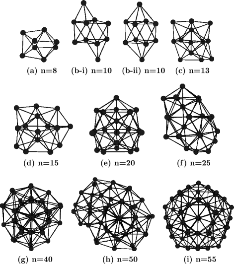
Figure 2: The ground–state geometries of the Na_n ($n=8-55$) clusters.

Figure 3: The deformation parameter, $\varepsilon_{def}$, of the ground–state geometries as a function of cluster size.

Figure 4: The eigenvalue spectra of their ground–state of Na_n ($n-8-50$) cluster as a function cluster size. The numbers on the right show the degeneracy of that level.

The lowest–energy geometries of sodium clusters are shown in Fig. 2. First, we note that the equilibrium geometries of Na₈, Na₁₃ and Na₂₀, obtained by us, are in agreement with those reported by Röthlisberger et al. Ursula The ground–state geometry of Na₈ (Fig. 2(a)) is a dodecahedron. One of its low–energy isomer is an antiprism ($\Delta~{}E=0.04$ eV). These two structures play a crucial role in the finite temperature behavior of this cluster. We find two nearly degenerate structures for Na₁₀, namely a bicapped dodecahedron (Fig. 2(b–i)) and a bicapped antiprism (Fig. 2(b–ii)). Röthlisberger et al. Ursula have found the bicapped dodecahedron to be unstable. However, we computed the vibrational spectra for both geometries and found the structures to be stable. The clusters, Na₁₃ (Fig. 2(c)) and Na₁₅ (Fig. 2(d)), exhibit capped pentagonal bipyramidal structures as their lowest–energy configurations. The ground–state geometry of Na₂₀ (Fig. 2(e)) is a fivefold capped icosahedron, with two atoms capping the icosahedral faces on the central plane. We find a capped double icosahedron to be about 0.11 eV higher in energy than the ground–state. The lowest–energy structure of Na₂₅ has not been previously reported. It may be described as capped double icosahedron with growth on one side, leading to a distorted non–spherical structure, as shown in Fig. 2(f). The ground–state geometry for Na₄₀, shown in Fig. 2(g), agrees with the one reported by Manninen et al. Manninen It consists of three decahedra capped by rest of the atoms. The structure is compact and retains the five–fold symmetry. The ground–state geometry of Na₅₀, shown in Fig. 2(h), is highly asymmetric. It can be seen from figure 2 that a growth towards 50–atom structure starting from symmetric Na₄₀ makes the structure non–spherical and asymmetric, which is similar as seen for Na₂₅ cluster. Finally, the ground–state geometry of Na₅₅ is a slightly distorted double Mackay icosahedron. It is the most spherical structure and is noted for the sake of completeness. Na55-142

We have also examined the eigenvalue spectra and the shapes of the ground–state geometries of these clusters, as shown in Figs. 4 and 3, respectively. The shape deformation parameter, $\varepsilon_{def}$, plotted in Fig. 3, for the ground–state geometries of all the clusters show that Na₂₀, Na₄₀ and Na₅₅ are nearly spherical, while Na₂₅ and Na₅₀ are deformed. This behavior is also reflected in the eigenvalue spectra of these clusters. The eigenvalue spectra of Na₂₀, Na₄₀ and Na₅₅ clusters (see Fig. 4), having nearly spherical geometries, conforms the jellium description. For instance, Na₅₅ shows a jellium–like behavior with s, p, d, … shell structure. However, for systems such as Na₂₅ and Na₅₀, due to the disordered nature of the ground–state geometries, the degeneracy in the eigenvalue spectra is lifted, thereby leading to a continuous spectra.

Figure 5: The normalized specific–heat as a function of temperature. $C_{0}=(3N-9/2)k_{B}$ is the zero–temperature classical limit of the rotational plus vibrational canonical specific–heat

.

III.2 Thermodynamics

The thermodynamic behavior is studied by analyzing several indicators. We have calculated the specific–heat, caloric curve, Lindemann criterion ($\delta_{rms}$) as a function of temperature for each cluster. These are shown in Figs. 5, 6 and 7, respectively. The melting temperatures, $T_{m}$, taken as the temperature corresponding to the peak in the specific–heat curve, are shown in Fig. 8.

Figure 6: The averaged potential energy (caloric curve) as a function of temperature.

Figure 7: The root–mean–square bond length fluctuation ($\delta_{rms}$) as a function of temperature.

Figure 8: The melting temperature as a function of size. The melting temperature in bulk (T_m[Bulk]) is 370 K is shown with the horizontal line.

Figure 9: The deviation of total energy from that of the harmonic limit plotted as a function of temperature. The error bar is the standard error at each temperature.

The examination of thermodynamic indicators as a function of cluster size reveals interesting trends. It may be seen that the clusters of sizes 8 and 10, do not show any recognizable peak in the heat capacities. This is also reflected in the caloric curves which increase continuously. While the peak is rather broad for $n=$ 13–20, it progressively becomes narrower as the size increases, and at $n=$ 92, a rather sharp peak with a width of the order of 30 K is observed. The caloric curve (Fig. 6) and the $\delta_{rms}$ (Fig. 7) for larger clusters, viz. $n=$ 40, 55, and 92, clearly show distinct solidlike, liquidlike and transition regions. Interestingly, the melting temperatures depicted in Fig. 8 show irregular pattern with the maximum variation of about 60 K. High melting temperatures are observed in two clusters: Na₄₀ and Na₅₅, which are very symmetric; Na₄₀ exhibiting electronic closure and Na₅₅ representing a geometrically closed system. We plot $\delta E$ in Fig. 9, which is an indicator of anharmonicity in the system. It is clear from the figure that for the clusters with $n\geq$ 40, it is possible to distinguish a temperature region ($<$200 K) showing harmonic behavior. In contrast to this, the smaller clusters change from harmonic to anharmonic behavior nearly continuously. The most remarkable observation concerns the trends in the specific–heat curve and other indicators for sizes $n=$ 40, 50 and 55. In spite of a well–defined peak in the specific–heat curves for Na₄₀ and Na₅₅, the Na₅₀ cluster shows a rather broad structure, similar to that seen in smaller clusters. This size–sensitive behavior is discussed further below.

Thus, all the indicators, like the specific–heat, the caloric curve, $\delta_{rms}$ and $\delta E$ clearly show that small clusters ($n=$ 8, 10) do not undergo any melting–like transition. The examination of their ionic motion indicates that over the entire range of the temperatures the motion is dominated by isomer hopping. This is in agreement with the observation by Manninen et al. Manninen However, these results are in contrast with the SMA and tight binding calculations of Calvo et al. Calvo , and the Car–Parrinello orbital free calculations of Aguado et al. Aguado Recall that these calculations, though are not in agreement with each other, show distinct peaks (broader in case of SMA) in the heat capacities of these clusters. Our simulations further show the smaller clusters to be dissociated at about 750 K. Our results for Na₁₃ and Na₂₀ are also in disagreement with those by Calvo et al. Calvo They calculated the canonical heat capacity of Na₁₃, using an icosahedron for SMA calculations and a pentagonal structure with $C_{1}$ symmetry for TB calculations as the ground–state geometries. While the heat capacity with the SMA potential exhibited a single prominent peak, that of TB calculation showed a premelting feature. They attributed this difference to the difference in the ground–state geometries. They further found such premelting feature in the heat capacity of Na₂₀ cluster, for which they used a capped double icosahedron as the lowest energy structure. However, our calculations show that this structure is about 0.1 eV higher than the ground–state structure obtained by us for Na₂₀. Thus, the differences in the specific–heat may be also caused by the differences in the ground–state geometries. The $\delta_{rms}$ for all the clusters (Fig. 7) clearly shows that for smaller systems ($n<$ 40), it increases almost continuously, whereas for larger ones, a sharp rise is seen that corresponds to the peak in the specific–heat. The behavior of $\delta E$ is, as noted earlier, consistent with this. We have also calculated a quantity $\delta E_{pot}$ defined as the difference of average potential energy of the melted cluster with respect to the ground–state structure at $T=0$ K. Schmidt et al.schmidt-na-dE have inferred from the experimental caloric curve that the melting temperature is strongly influenced by such an energy contribution. They showed further that $T_{m}$ follows closely the variation in energy difference between solid and liquid as a function of the cluster size. To examine this feature, we plot the potential energy difference between solidlike–state and liquidlike–state shown in Fig. 10. For this purpose, we have taken the high temperature as 300 K for $n=$ 13, 15, 20, 25, and 50, 350 K for $n=$ 40, 55, which are about 50 K to 70 K higher than the melting temperature of the respective clusters. It can be immediately seen that the variation of $\delta E_{pot}$ follows that of the melting temperature (Fig. 8), clearly indicating that the melting transition is mainly driven by energy contribution.

Figure 10: The difference of average potential energy $\delta E_{pot}$ between solid–state and liquid–state as a function of size.

III.3 Na₄₀ $\cdot$ Na₅₀ $\cdot$ Na₅₅

Now, we turn our discussion to the most remarkable observation concerning the trends in the specific–heat in going from $n=$ 40 to $n=$ 55. As mentioned earlier, while Na₄₀ and Na₅₅ show well–defined peaks in the specific–heat curve (peak for Na₅₅ being much sharper), the peak for Na₅₀ is rather flat and is almost similar to that of the smaller clusters (say, $n=$ 13–20). We note that Na₅₀, being larger than Na₄₀, is expected to show slightly better melting transition. Interestingly, what is seen is exactly the opposite. It may be noted that such peculiar size–sensitivity has been observed experimentally in two systems, namely clusters of gallium (Ga${}_{n}^{+}$, $n=$ 30–50 and 55) jarrold-ga2 and clusters of aluminum (Al${}_{n}^{+}$, $n=$ 49–62) jarrold-al . For instance, in case of Ga clusters the heat capacity for $n=$ 30 shows a flat curve without a peak. For $n=$ 31 it shows a remarkably sharp peak. Interestingly, addition of one more atom (i.e. $n=$ 32) diminishes this peak making the heat capacity nearly flat. We believe this behavior to be generic as it has not only been observed experimentally in case of gallium clusters but also for aluminum cluster and theoretically for sodium clusters in the present simulations.

We note certain peculiar characteristics of the thermodynamic properties of Na₄₀, Na₅₀, and Na₅₅. We find the melting temperature of Na₅₀ to be about 60 K lower that that of Na₄₀ and Na₅₅. The $\delta_{rms}$ for Na₅₀ exhibits gradual increase in the temperature range of 100 K to 300 K. Further, the energy deviation $\delta E$ for Na₅₀, as seen in Fig. 9, starts to increase continuously at about 100 K to up to about 400 K, indicating a continuous change from harmonic behavior to anharmonic one. This behavior of Na₅₀ is in contrast with that of Na₄₀ and Na₅₅, where the change is seen in a smaller temperature width (of about 30–40 K) around the melting temperature. In order to bring out the origin of this phenomena, we examine the nature of the ground–state geometries for these three clusters. Na₄₀ and Na₅₅ are very symmetric structures having almost five–fold symmetry. The values of the shape deformation parameter, $\varepsilon_{def}$, shown in Fig. 3, clearly indicate that they are nearly spherical structures. Further, the eigenvalue spectra of the ground–state geometries of Na₄₀ and Na₅₅ clusters also show this symmetry, conforming the jellium model. However, the eigenvalue spectrum of Na₅₀ is very different from those of Na₄₀ and Na₅₅, in the sense that there are levels in the energy gaps leading to a more uniform spectrum. In this sense, Na₄₀ and Na₅₅ are ordered, i.e. more symmetric, and Na₅₀ is amorphous.

Figure 11: The distance from the center of mass for the ground–state geometries of Na₅₀ and Na₅₅.

In Fig. 11, we show the distances from the center of mass of all the atoms in the ground–state geometries of Na₅₀ and Na₅₅ . Clearly, the ordered geometric shell structure of Na₅₅ is destroyed when five atoms are removed. We believe that the nature of ground–state geometry of the cluster has a significant effect on its melting characteristics. An ordered or symmetric cluster, like Na₄₀ and Na₅₅, is expected to give rise to a well–defined peak in the heat capacity, while an amorphous and disordered clusters, like Na₂₅ and Na₅₀, may lead to a continuous melting transition.

IV Summary

We have investigated the thermodynamics properties of small sodium clusters, Na_n, in the size range of 8 to 55, using ab initio molecular dynamics with simulation time of 1.3–1.8 $ns$ per cluster. We have analyzed several thermodynamic indicators such as the specific–heat, caloric curve, Lindemann criterion, and the deviation energy $\delta E$ to understand the melting characteristics in these clusters. We observe irregular variation in the melting temperatures as a function of size, which has also been seen in experiments by Haberland and coworkers for larger clusters. The reduction of about 30 % than the bulk value in melting temperature of sodium clusters, seen in experiment is also observed here. Further, we find a strong correlation between the ground–state geometry and the finite temperature characteristics of the sodium clusters. If a cluster has an ordered geometry, it is likely to show a relatively sharp melting transition. However, a cluster having a disordered geometry is expected to exhibit a broad peak in the specific–heat curve, indicating a poorly–defined melting transition. The size–sensitivity in the melting transition, seen in experiments by Breaux et al. jarrold-ga2 ; jarrold-al , is observed for the case of sodium clusters in the size range of 40 to 50. The calculation of potential energy difference between solidlike state and liquidlike state reveals that the melting transition is mainly driven by the energy contribution and the entropy has a minor role in melting phenomena.

V Acknowledgments

It is a pleasure to acknowledge C–DAC (Pune) for the supercomputing facilities. We also acknowledge partial assistance from the Indo–French Center by providing the computational support. One of us (SC) acknowledges financial support from the Center for Modeling and Simulation, University of Pune and the Indo–French Center for Promotion for Advance Research (IFCPAR). We would like to thank Sailaja Krishnamurty for a number of useful discussions.

References

- (1) M. Schmidt, R. Kusche, B. von Issendorff, and H. Haberland, Nature (London) 393, 238 (1998); M. Schmidt and H. Haberland, C. R. Physique 3, 327, (2002); H. Haberland, T. Hippler, J. Donges, O. Kostko, M. Schmidt and B. von Issendorff. Phys. Rev. Lett. 94, 035701 (2005).
- (2) A. A. Shvartsburg and M. F. Jarrold, Phys. Rev. Lett. 85, 2530 (2000)
- (3) G. A. Breaux, R. C. Benirschke, T. Sugai, B. S. Kinnear, and M. F. Jarrold, Phys. Rev. Lett. 91, 215508 (2003).
- (4) K. Joshi, D. G. Kanhere, and S. A. Blundell, Phys. Rev. B 66, 155329 (2002); ibid. 67, 235413 (2003).
- (5) S. Chacko, K. Joshi, D. G. Kanhere, and S. A. Blundell, Phys. Rev. Lett. 92, 135506 (2004).
- (6) G. A. Breaux, D. A. Hillman, C. M. Neal, R. C. Benirschke, and M. F. Jarrold, J. Am. Chem. Soc. 126, 8628 (2004).
- (7) G. A. Breaux, C. M. Neal, B. Cao, and M. F. Jarrold, Phys. Rev. Lett. 94, 173401 (2005).
- (8) F. Calvo and F. Spiegelmann, J. Chem. Phys. 112, 2888 (2000).
- (9) Y. Li and, E. Blaisten-Barojas, and D. A. Papaconstantopoulos, Phys. Rev. B 57, 15519 (1998).
- (10) S. Chacko, D. G. Kanhere, and S. A. Blundell, Phys. Rev. B 71, 155407 (2005).
- (11) W. Kohn and L. J. Sham, Phys. Rev. 140, A1133 (1965).
- (12) A. Rytkönen, H. Häkkinen, and M. Manninen, Phys. Rev. Lett. 80, 3940 (1998).
- (13) A. Aguado, J. M. López, J. A. Alonso, and M. J. Stott, J. Chem. Phys. 111, 6026 (1999).
- (14) A. Vichare, D. G. Kanhere, and S. A. Blundell, Phys. Rev. B 64, 045408 (2001).
- (15) M. C. Payne, M. P. Teter, D. C. Allan, T. A. Arias, and J. D. Joannopoulos, Rev. Mod. Phys. 64, 1045 (1992)
- (16) D. Vanderbilt, Phys. Rev. B 41, 7892 (1990)
- (17) Vienna Ab initio Simulation Package (VASP), Technishe Universität Wien, 1999
- (18) Z. Li and H. A. Scheraga, Proc. Natl. Acad. Sci. U.S.A. 84, 6611 (1987); D. J. Wales and J. P. K. Doye, J. Phys. Chem. A 101, 5111 (1997).
- (19) R. G. Parr and W. Yang, Oxford University press, New York, 1989.
- (20) In our earlier work (see Ref. Na55-142, ), we have verified that an energy cutoff of 3.6 Ry is sufficient. It gives results as accurate an the nearly all–electron projected–augmented wave method (see Ref. paw, ), taking only 1 electrons in the core with an energy cutoff of 51 Ry. The Na2 binding energy and bond–length by these two methods differ by less than 3%.
- (21) G. Kresse and D. Joubert, Phys. Rev. B 59, 1578 (1999); P. E. Blöchl, Phys Rev. B 50, 17 953 (1994).
- (22) A. M. Ferrenberg and R. H. Swendsen, Phys. Rev. Lett. 61, 2635 (1988); P. Labastie and R. L. Whetten, ibid. 65, 1567 (1990).
- (23) Feng-chuan Chuang, C. Z. Wang, Serdar Öğüt, James R. Chelikowsky, and K. M. Ho, Phys. Rev. B 69, 165408 (2004).
- (24) U. Röthlisberger and W. Andreoni, J. Chem. Phys. 94, 8129 (1991).
- (25) M. Schmidt, J. Donges, Th. Hippler, and H. Haberland, Phys. Rev. Lett. 90, 103401 (2003).