Scaling in critical random Boolean networks

Abstract

We derive mostly analytically the scaling behavior of the number of nonfrozen and relevant nodes in critical Kauffman networks (with two inputs per node) in the thermodynamic limit. By defining and analyzing a stochastic process that determines the frozen core we can prove that the mean number of nonfrozen nodes scales with the network size $N$ as $N^{2/3}$, with only $N^{1/3}$ nonfrozen nodes having two nonfrozen inputs. We also show the probability distributions for the numbers of these nodes. Using a different stochastic process, we determine the scaling behavior of the number of relevant nodes. Their mean number increases for large $N$ as $N^{1/3}$, and only a finite number of relevant nodes have two relevant inputs. It follows that all relevant components apart from a finite number are simple loops, and that the mean number and length of attractors increases faster than any power law with network size.

1 Introduction

Random Boolean networks are often used as generic models for the dynamics of complex systems of interacting entities, such as social and economic networks, neural networks, and gene or protein interaction networks Kauffman et al. (2003). The simplest and most widely studied of these models was introduced in 1969 by Kauffman Kauffman (1969) as a model for gene regulation. The system consists of $N$ nodes, each of which receives input from $K$ randomly chosen other nodes. The network is updated synchronously, the state of a node at time step $t$ being a Boolean function of the states of the $K$ input nodes at the previous time step, $t-1$. The Boolean updating functions are randomly assigned to every node in the network, and together with the connectivity pattern they define the realization of the network. For any initial condition, the network eventually settles on a periodic attractor. Of special interest are critical networks, which lie at the boundary between a frozen phase and a chaotic phase Derrida and Pomeau (1986); Derrida and Stauffer (1986). In the frozen phase, a perturbation at one node propagates during one time step on an average to less than one node, and the attractor lengths remain finite in the limit $N\to\infty$. In the chaotic phase, the difference between two almost identical states increases exponentially fast, because a perturbation propagates on an average to more than one node during one time step Aldana-Gonzalez et al. (2003).

The nodes of a critical network can be classified according to their dynamics on an attractor. First, there are nodes that are frozen on the same value on every attractor. Such nodes give a constant input to other nodes and are otherwise irrelevant. They form the frozen core of the network. Second, there are nodes whose outputs go only to irrelevant nodes. Though they may fluctuate, they are also classified as irrelevant since they act only as slaves to the nodes determining the attractor period. Third, the relevant nodes are the nodes whose state is not constant and that control at least one relevant node. These nodes determine completely the number and period of attractors. If only these nodes and the links between them are considered, these nodes form loops with possibly additional links and chains of relevant nodes within and between loops. The recognition of the relevant elements as the only elements influencing the asymptotic dynamics was an important step in understanding the attractors of Kauffman networks. The behavior of the frozen core was first studied by Flyvbjerg Flyvbjerg (1988). Then, in an analytical study of $K=1$ networks Flyvbjerg and Kjaer Flyvbjerg and Kjær (1988) introduced the concept of relevant elements (though without using this name). The definition of relevant elements that we are using here was given by Bastolla and Parisi Bastolla and Parisi (1998a, b). They gained insight into the properties of the attractors of the critical networks by using numerical experiments based on the modular structure of the relevant elements. Finally, Socolar and Kauffman Socolar and Kauffman (2003) found numerically that for critical $K=2$ networks the mean number of nonfrozen nodes scales as $N^{2/3}$, and the mean number of relevant nodes scales as $N^{1/3}$. The same result is hidden in the analytical work on attractor numbers by Samuelsson and Troein Samuelsson and Troein (2003), as was shown in Drossel (2005).

In this work, we go a step further by deriving these power laws analytically for a more general class of networks, and by showing the asymptotic probability distribution of nonfrozen and relevant nodes in terms of scaling variables. We also obtain results for the number of nonfrozen nodes with two nonfrozen inputs, and for the number of relevant nodes with two relevant inputs. The outline of this paper is the following. In the next section we define the class of networks that we are investigating. In Section 3, we introduce a stochastic process that determines the frozen core of the network starting from the nodes whose outputs are entirely independent of their inputs. Then, in Section 4, we analyze the Langevin and Fokker-Planck equations that correspond to this stochastic process and that lead to the scaling behavior of the number of nonfrozen nodes. In order to identify the relevant nodes among the nonfrozen ones, we introduce in Section 5 another stochastic process. This process also enables us to find their scaling behavior. Finally, we discuss in the last section the implications of our results.

2 Critical $K=2$ networks

The networks we are studying in this paper are the $K=2$ critical networks. In these networks each node has 2 randomly chosen inputs. The 16 possible update functions are shown in table 1.

In	$\mathcal{F}$		${\mathcal{C}}_{1}$				${\mathcal{C}}_{2}$								$\mathcal{R}$
00	1	0	0	1	0	1	1	0	0	0	0	1	1	1	1	0
01	1	0	0	1	1	0	0	1	0	0	1	0	1	1	0	1
10	1	0	1	0	0	1	0	0	1	0	1	1	0	1	0	1
11	1	0	1	0	1	0	0	0	0	1	1	1	1	0	1	0

Table 1: The 16 update functions for nodes with 2 inputs. The first column lists the 4 possible states of the two inputs, the other columns represent one update function each, falling into four classes.

The update functions fall into four classes Aldana-Gonzalez et al. (2003). In the first class, denoted by $\mathcal{F}$, are the frozen functions, where the output is fixed irrespectively of the input. The class ${\mathcal{C}}_{1}$ contains those functions that depend only on one of the two inputs, but not on the other one. The class ${\mathcal{C}}_{2}$ contains the remaining canalizing functions, where one state of each input fixes the output. The class $\mathcal{R}$ contains the two reversible update functions, where the output is changed whenever one of the inputs is changed. Critical networks are those where a change in one node propagates to one other node on an average. A change propagates with probability $1/2$ to a node that has a canalizing update function $\mathcal{C}_{1}$ or $\mathcal{C}_{2}$, with probability zero to a node that has a frozen update function, and with probability 1 to a node that has a reversible update function. Consequently, if the frozen and reversible update functions are chosen with equal probability, the network is critical. Usually, only those models are considered where all 16 update functions receive equal weight. We here consider the larger set of models where the frozen and reversible update functions are chosen with equal (and nonzero) probability, and where the remaining probability is divided between the $\mathcal{C}_{1}$ and $\mathcal{C}_{2}$ functions. Those networks that contain only $\mathcal{C}_{1}$ functions are different from the remaining ones. Since all nodes respond only to one input, the link to the second input can be cut, and we are left with a critical $K=1$ network, which was already discussed in Flyvbjerg and Kjær (1988); Drossel et al. (2005); Drossel (2005) and will not be discussed here. All the other models, where the weight of the $\mathcal{C}_{1}$ functions is smaller than 1, fall into the same class Drossel (2005). The treatment presented in the following, is based on the existence of nodes with frozen functions, and it therefore applies to all critical models with a nonzero fraction of frozen functions. Networks with only canalyzing functions have to be discussed separately.

Let $N_{f}$ be the number of nodes with a frozen function, $N_{r}$ the number of nodes with a reversible function and $N_{c_{1}}$ and $N_{c_{2}}$ the number of nodes with a $\mathcal{C}_{1}$ and a $\mathcal{C}_{2}$ function. We define the systems we are going to consider through parameters $\alpha=N_{c_{1}}/N$, $\beta=N_{r}/N=N_{f}/N$, $\gamma=N_{c_{2}}/N$. These parameters give the fraction of each type of nodes in the network. In the next two sections, we determine the properties of the frozen core in the large $N$ limit by starting from the nodes with a frozen function.

3 A stochastic process that leads to the frozen core

We consider the ensemble of all networks of size $N$ and with fixed parameters $\alpha,\beta,\gamma$. All nodes with a frozen update function are certainly part of the frozen core. We now construct the frozen core by determining stepwise all those nodes that become frozen due to the influence of a frozen node. In the language of Socolar and Kauffman (2003), this process determines the “clamped” nodes. Initially, we place the nodes in four containers labelled $\mathcal{F}$, $\mathcal{C}_{1}$, $\mathcal{C}_{2}$, and $\mathcal{R}$. These containers contain $N_{f}$, $N_{c_{1}}$, $N_{c_{2}}$, and $N_{r}$ nodes initially. Since these numbers change during our stochastic process, we denote the initial values as $N_{f}^{ini}$, $N_{c_{1}}^{ini}$, $N_{c_{2}}^{ini}$, and $N_{r}^{ini}$, and the total number of nodes as $N^{ini}$. We treat the nodes in container $\mathcal{C}_{1}$ as nodes with only one input and with the update functions “copy” or “invert”. The contents of the containers will change with time. The “time” we are defining here is not the real time for the dynamics of the system. Instead, it is the time scale for a stochastic process that we use to determine the frozen core. During one time step, we remove one node from the container $\mathcal{F}$ and determine all those nodes, to which this node is an input. A node in container $\mathcal{C}_{1}$ chooses this node as an input with probability $1/N$. It then becomes a frozen node. We therefore move each node of container $\mathcal{C}_{1}$ with probability $1/N$ into the container $\mathcal{F}$. A node in container $\mathcal{C}_{2}$ chooses the selected frozen node as an input with probability $2/N$. With probability $1/2$, it then becomes frozen, because the frozen node is with probability $1/2$ in the state that fixes the output of a $\mathcal{C}_{2}$-node. If the $\mathcal{C}_{2}$-node does not become frozen, it becomes a $\mathcal{C}_{1}$-node. We therefore move each node of container $\mathcal{C}_{2}$ during the first time step with probability $1/N$ into the container $\mathcal{F}$, and with probability $1/N$ into the container $\mathcal{C}_{1}$. Finally, a node in container $\mathcal{R}$ chooses the selected frozen node as an input with probability $2/N$ and becomes a $\mathcal{C}_{1}$-node. We therefore move each node of container $\mathcal{R}$ during the first time step with probability $2/N$ into the container $\mathcal{C}_{1}$. In summary, the total number of nodes, $N$, decreases by one during one time step, since we remove one node from container $\mathcal{F}$, and some nodes move to a different container. The removed nodes are those frozen nodes for which we already have determined whose input they are. Then, we take the next frozen node out of container $\mathcal{F}$ and determine its effect on the other nodes. We repeat this procedure until we cannot continue because either container $\mathcal{F}$ is empty, or because all the other containers are empty. If container $\mathcal{F}$ becomes empty, we are left with the nonfrozen nodes. We shall see below that most of the remaining nodes are in container $\mathcal{C}_{1}$, with the proportion of nodes left in containers $\mathcal{C}_{2}$ and $\mathcal{R}$ vanishing in the limit $N^{ini}\to\infty$. Then, the nonfrozen nodes can be connected to a network by choosing the input(s) to every node at random from the other remaining nodes. If all containers apart from container $\mathcal{F}$ are empty at the end, the entire network becomes frozen. This means that the dynamics of the network go to the same fixed point for all initial conditions.

Let us first describe this process by deterministic equations that neglect fluctuations around the average change of the number of nodes in the different containers. As long as all containers contain large numbers of nodes, these fluctuations are negligible, and the deterministic description is appropriate. The average change of the node numbers in the containers during one time step is

$$\Delta N_{r} = -\frac{2N_{r}}{N}$$

$$\Delta N_{c_{2}} = -\frac{2N_{c_{2}}}{N}$$

$$\Delta N_{c_{1}} = -\frac{N_{c_{1}}}{N}+\frac{N_{c_{2}}}{N}+\frac{2N_{r}}{N}$$ (1)

$$\Delta N_{f} = -1+\frac{N_{c_{1}}}{N}+\frac{N_{c_{2}}}{N}$$

$$\Delta N = -1$$

The number of nodes in the containers, $N$, can be used instead of the time variable, since it decreases by one during each step. The equation for $N_{r}$ can then be solved by going from a difference equation to a differential equation,

$$\frac{\Delta N_{r}}{\Delta N}\simeq\frac{dN_{r}}{dN}=-\frac{2N_{r}}{N}\,,$$

which has the solution

$$N_{r}=N^{2}\frac{N_{r}^{ini}}{(N^{ini})^{2}}\,.$$ (2)

Similarly, we find

$$N_{c_{2}} = N^{2}\frac{N_{c_{2}}^{ini}}{(N^{ini})^{2}}$$

$$N_{f} = N\frac{N_{f}^{ini}-N_{r}^{ini}}{N^{ini}}+N^{2}\frac{N_{r}^{ini}}{(N^{ini})^{2}}$$

$$N_{c_{1}} = N\frac{N_{c_{1}}^{ini}+N_{c_{2}}^{ini}+2N_{r}^{ini}}{N^{ini}}-2N^{2}\frac{N_{r}^{ini}+N_{c_{2}}^{ini}}{(N^{ini})^{2}}\,.$$ (3)

For $N_{f}^{ini}<N_{r}^{ini}$, we obtain $N_{f}=0$ at a nonzero value of $N$, and the number of nonfrozen nodes is proportional to $N^{ini}$. We are in the chaotic phase. For $N_{f}^{ini}>N_{r}^{ini}$, the values $N_{r}$ and $N_{c_{2}}$ will sink below 1 when $N$ becomes of the order $\sqrt{N^{ini}}$. For smaller $N$, there are only $\mathcal{F}$ and $\mathcal{C}_{1}$ nodes left, and the second term contributing to $N_{f}$ and $N_{c_{1}}$ in (3) can be neglected compared to the first one. When $N_{f}$ falls below 1, there remain $N_{c_{1}}=\frac{N_{c_{1}}^{ini}+N_{c_{2}}^{ini}+2N_{r}^{ini}}{N_{f}^{ini}-N_{r}^{ini}}$ nodes of type $\mathcal{C}_{1}$. The network is essentially frozen, with only a finite number of nonfrozen nodes in the limit $N^{ini}\to\infty$. If we now choose the inputs for these nodes, we obtain simple loops with trees rooted in the loops. This property of the frozen phase was also found in Socolar and Kauffman (2003).

For the critical networks that this paper focuses on, we have $N_{f}^{ini}=N_{r}^{ini}=\beta N^{ini}$, and the stochastic process stops at $N_{f}=1=\beta{N^{2}}/{N^{ini}}$. This means that

$$N^{end}=\sqrt{\frac{N^{ini}}{\beta}}\,.$$ (4)

The number of nonfrozen nodes would scale with the square root of the network size if the deterministic approximation to the stochastic process was exact. We shall see below that including fluctuations changes the exponent from $1/2$ to $2/3$. The final number of $\mathcal{C}_{2}$-nodes for the deterministic process for the critical networks is $\gamma/\beta$, which is independent of network size, and the final number of $\mathcal{R}$-nodes vanishes due to $N_{r}=N_{f}$. We shall see below that the fluctuations change these two results to a $(N^{ini})^{1/3}$-dependence.

Introducing $n=N/N^{ini}$ and $n_{j}=N_{j}/N^{ini}$ for $j=r,f,c_{1},c_{2}$, equations (3) simplify to (using $N_{r}^{ini}=N_{f}^{ini}$)

$$n_{r} = \beta n^{2}=n_{f}$$

$$n_{c_{2}} = \gamma n^{2}$$

$$n_{c_{1}} = n-2\beta n^{2}-\gamma n^{2}\,.$$

This means that our stochastic process remains invariant (in the deterministic approximation) when the initial number of nodes in the containers and the time unit are all multiplied by the same factor. For small $n$, the majority of nodes are in container $\mathcal{C}_{1}$, since $n_{c_{1}}=n-\mathcal{O}(n^{2})$. Now, if we choose a sufficiently large $N^{ini}$, $n$ reaches any given small value while $N_{f}=N_{r}=\beta n^{2}N^{ini}$ is still large enough for a deterministic description. We can therefore assume that for sufficiently large networks $N_{f}/N=\beta n$ becomes small before the effect of the noise becomes important. This assumption will simplify our calculations below.

4 The effect of fluctuations

The number of nodes in container $\mathcal{C}_{1}$ that choose a given frozen node as an input is Poisson distributed with a mean $N_{c_{1}}/N$ and a variance $N_{c_{1}}/N$. We now assume that $n$ is small at the moment where noise becomes important, i.e., that the variance of the noise $N_{c_{1}}/N=n_{c_{1}}/n=1-(2\beta+\gamma)n=1-\mathcal{O}(n)$ is unity. The number of nodes in containers $\mathcal{C}_{2}$ and $\mathcal{R}$ that choose a given frozen node as an input is Poisson distributed with a mean and a variance $2(N_{c_{2}}+N_{r})/N$. The fluctuation around the mean can be neglected as this noise term is very small compared to $N_{r}$ and $N_{c_{2}}$, the final values of which are large for sufficiently large $N^{ini}$. We therefore obtain the stochastic version of equations (1)

$$\Delta N_{r} = -\frac{2N_{r}}{N}$$

$$\Delta N_{c_{2}} = -\frac{2N_{c_{2}}}{N}$$

$$\Delta N_{f} = -\frac{N_{r}}{N}-\frac{N_{f}}{N}+\xi$$

$$\Delta N = -1$$ (5)

The random variable $\xi$ has zero mean and unit variance. As long as the $n_{j}$ change little during one time step, we can summarize a large number $T$ of time steps into one effective time step, with the noise becoming Gaussian distributed with zero mean and variance $T$. Exactly the same process would result if we summarized $T$ time steps of a process with Gaussian noise of unit variance. For this reason, we can choose the random variable $\xi$ to be Gaussian distributed with unit variance.

Compared to the deterministic case, the equations for $N_{r}$ and $N_{c_{2}}$ are unchanged, and we have again $N_{r}=N^{2}N_{r}^{ini}/(N^{ini})^{2}$ and $N_{c_{2}}=N^{2}N_{c_{2}}^{ini}/(N^{ini})^{2}$. Inserting the solution for $N_{r}$ into the equation for $N_{f}$, we obtain

$$\frac{dN_{f}}{dN}=\frac{N_{f}}{N}+\frac{\beta N}{N^{ini}}+\xi$$ (6)

with the step size $dN=1$ and $\langle\xi^{2}\rangle=1$. (In the continuum limit $dN\to 0$ the noise correlation becomes $\langle\xi(N)\xi(N^{\prime})\rangle=\delta(N-N^{\prime})$). This is a Langevin-equation, and we will now derive the corresponding Fokker-Planck-equation. Let $P(N_{f},N)$ be the probability that there are $N_{f}$ nodes in container $\mathcal{R}$ at the moment where there are $N$ nodes in total in the containers. This probability depends on the initial node number $N_{ini}$, and on the parameter $\beta$. The sum

$$\sum_{N_{f}=1}^{\infty}P(N_{f},N)\simeq\int_{0}^{\infty}P(N_{f},N)dN_{f}$$

is the probability that the stochastic process is not yet finished, i.e. the probability that $N_{f}$ has not yet reached the value 0 at the moment where the total number of nodes in the containers has decreased to the value $N$. Since systems that have reached $N_{f}=0$ are removed from the ensemble, we have to impose the absorbing boundary condition $P(0,N)=0$. Let $g(\Delta N_{f}|N_{f},N)$ denote the probability that $N_{f}$ decreases by $\Delta N_{f}$ during the next step, given the values of $N_{f}$ and $N$.

We have

$$P(N_{f},N-1)=$$

$$\int_{0}^{\infty}P(N_{f}+\Delta N_{f},N)g(\Delta N_{f}|N_{f}+\Delta N_{f},N)d(\Delta N_{f})$$

$$=\int_{0}^{\infty}\Bigl{[}P(N_{f},N)g(\Delta N_{f}|N_{f},N)$$

$$\quad+\frac{\partial}{\partial N_{f}}(P(N_{f},N)g(\Delta N_{f}|N_{f},N))\Delta N_{f}$$

$$\quad+\frac{\partial^{2}}{2\partial^{2}N_{f}^{2}}(P(N_{f},N)g(\Delta N_{f}|N_{f},N))(\Delta N_{f})^{2}$$

$$\quad+\ldots\Bigr{]}d(\Delta N_{f})$$

$$=P(N_{f},N)+\frac{\partial}{\partial N_{f}}(P(N_{f},N)\langle\Delta N_{f}\rangle)+$$

$$\quad\frac{\partial^{2}}{2\partial N_{f}^{2}}(P(N_{f},N)\langle(\Delta N_{f})^{2}\rangle)+\ldots$$

The mean change $\langle\Delta N_{f}\rangle$ during one step is $\langle\Delta N_{f}\rangle=\frac{N_{f}}{N}+\frac{\beta N}{N^{ini}}$, and the mean square change is $\langle(\Delta N_{f})^{2}\rangle\simeq 1$.

This gives the Fokker-Planck equation for our stochastic process

$$-\frac{\partial P}{\partial N}=\frac{\partial}{\partial N_{f}}\left(\frac{N_{f}}{N}+\frac{\beta N}{N^{ini}}\right)P+\frac{1}{2}\frac{\partial^{2}P}{\partial N_{f}^{2}}\,.$$ (7)

We introduce the variables

$$x=\frac{N_{f}}{\sqrt{N}}\hbox{ and }y=\frac{N}{(N^{ini}/\beta)^{2/3}}$$ (8)

and the function $f(x,y)=(N^{ini}/\beta)^{1/3}P(N_{f},N)$. We will see below that $f(x,y)$ does not depend explicitely on the parameters $N^{ini}$ and $\beta$ with this definition. The Fokker-Planck equation then becomes

$$y\frac{\partial f}{\partial y}+f+\left(\frac{x}{2}+y^{3/2}\right)\frac{\partial f}{\partial x}+\frac{1}{2}\frac{\partial^{2}f}{\partial x^{2}}=0\,.$$ (9)

Let $W(N)$ denote the probability that $N$ nodes are left at the moment where $N_{f}$ reaches the value zero. It is

$$W(N) = \quad\int_{0}^{\infty}P(N_{f},N)dN_{f}-\int_{0}^{\infty}P(N_{f},N-1)dN_{f}\,.$$

Consequently,

$$W(N) = \frac{\partial}{\partial N}\int_{0}^{\infty}P(N_{f},N)dN_{f}$$ (10)

$$= (N^{ini}/\beta)^{-1/3}\frac{\partial}{\partial N}\sqrt{N}\int_{0}^{\infty}f(x,y)dx$$

$$= (N^{ini}/\beta)^{-2/3}\frac{\partial}{\partial y}\sqrt{y}\int_{0}^{\infty}f(x,y)dx$$

$$\equiv (N^{ini}/\beta)^{-2/3}G(y)$$

with a scaling function $G(y)$. $W(N)$ must be a normalized function, $\int_{0}^{\infty}W(N)dN=\int_{0}^{\infty}G(y)dy=1$. This condition is independent of the parameters of the model, and therefore $G(y)$ and $f(x,y)$ are independent of them, too, which justifies our choice of the prefactor in the definition of $f(x,y)$. By integrating equation (9) over $x$ from 0 to infinity and by using $f(0,y)=f(\infty,y)=0$ we obtain

$$\sqrt{y}\frac{\partial}{\partial y}\sqrt{y}\int_{0}^{\infty}fdx-\frac{1}{2}\left.\frac{\partial f}{\partial x}\right|_{x=0}=0\,,$$

which gives us a second relation between $f(x,y)$ and $G(y)$:

$$\sqrt{y}G(y)=\frac{1}{2}\left.\frac{\partial f}{\partial x}\right|_{x=0}\,.$$ (11)

The mean number of nonfrozen nodes is

$$\bar{N}=\int_{0}^{\infty}NW(N)dN=(N^{ini}/\beta)^{2/3}\int_{0}^{\infty}G(y)ydy\,,$$ (12)

which is proportional to $(N^{ini}/\beta)^{2/3}$. We did not succeed in extracting an explicit expression for the function $G(y)$. It can be determined by running the stochastic process described by the equations (5) on the computer. The result is shown in Figure 1, and an almost perfect fit to this result is given by

$$G(y)\simeq 0.25e^{-y^{3}/2}(1-0.5\sqrt{y}+3y)/\sqrt{y}\,.$$ (13)

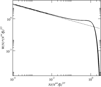
Figure 1: The function $W(N)(N^{ini}/\beta)^{2/3}$ vs $N/(N^{ini}/\beta)^{2/3}$ for $\beta=0.25$ and $N^{ini}=2^{16},2^{17},2^{18},2^{19},2^{20},2^{21}$. Furthermore, the graph contains a curve with $\beta=0.125,N=2^{16}$ and a curve with $\beta=0.5,N=2^{16}$. The curves all collapse, confirming the existence of a scaling function $G(y)$. The dashed line is a power law $\sim 1/\sqrt{N}$.

For small $y$, the data show a power law $G(y)\propto y^{-1/2}$. We can obtain this power law analytically by solving the Fokker-Planck equation (9) in the limit of small $y$. In this limit, the term proportional to $y^{3/2}$ can be dropped, and we have the simpler equation

$$y\frac{\partial f}{\partial y}+f+\frac{x}{2}\frac{\partial f}{\partial x}+\frac{1}{2}\frac{\partial^{2}f}{\partial x^{2}}=0\,.$$ (14)

The general solution has the form $f(x,y)=\sum_{\nu}c_{\nu}y^{\nu}f_{\nu}(x)$, with the functions $f_{\nu}$ satisfying

$$2(\nu+1)f_{\nu}+xf_{\nu}^{\prime}+f_{\nu}^{\prime\prime}=0\,.$$ (15)

The solution is

$$e^{\frac{x^{2}}{2}}f_{\nu}(x)=C_{1}H_{1+2\nu}\left(\frac{x}{\sqrt{2}}\right)+C_{2}\,{}_{1}F_{1}\left(-\nu-\frac{1}{2};\frac{1}{2};\frac{x^{2}}{2}\right)$$

with two constants $C_{1}$ and $C_{2}$, and with $H$ denoting the Hermitian functions, and ${}_{1}F_{1}$ the appropriate hypergeometric functions. We expect $f$ to be analytical in $y$ for small $y$, which means that $\nu=0,1,2,\dots$. For sufficiently small $y$, only the term $\nu=0$ contributes, and due to the absorbing boundary condition we have $C_{2}=0$. We obtain therefore for small $y$

$$f(x,y)=c_{0}xe^{-x^{2}/2}\,.$$ (16)

From our numerical result (13), together with (11), we find $c_{0}=0.5$. Inserting Eq. (16) into Eq. (10), we obtain for small $N$

$$W(N)=\left(\frac{N^{ini}}{\beta}\right)^{-1/3}\frac{c_{0}}{2\sqrt{N}}\,.$$ (17)

In Eq. (16), the function $f(x,y)$ is independent of $y$. This means that for sufficiently small $N$ the function $P(N_{f},N)$ depends only on the ratio $N_{f}/\sqrt{N}$. This is also confirmed by our computer simulations (see Fig. 2).

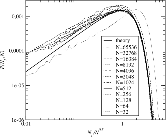
Figure 2: $P(N_{f},N)$ vs $N_{f}/\sqrt{N}$ for $N^{ini}=2^{21}$ and $\beta=1/4$ for different $N$. The thick solid line is the theoretical result Eq. (16), which is approached in the limit of small $N/(N^{ini})^{2/3}$.

We can obtain a set of solutions of Eq. (9) with the Ansatz $f(x,y)=\sum_{\nu}y^{\nu}\tilde{f}_{\nu}(z)$ with $z=x-y^{3/2}$. The resulting equation for $\tilde{f}_{\nu}$, is identical to Eq. (15) for $f_{\nu}$, which was valid for small $y$. However, an analytical expression for the function $G(y)$ can only be given if an expansion of the initial condition $P(N_{f},N)=\delta(N_{f}-\beta N^{ini})$ in terms of known solutions can be found.

The probability $W_{r}(N_{r})$ that $N_{r}$ nodes are left in container $\mathcal{R}$ at the moment where container $\mathcal{F}$ becomes empty, is obtained from the relation

$$N_{r}=N^{2}N_{r}^{ini}/(N^{ini})^{2}\,.$$

Defining

$$s=\frac{N_{r}}{(N^{ini}/\beta)^{1/3}}=y^{2}$$

and

$$F(s)=\frac{G(\sqrt{s})}{2\sqrt{s}}\,,$$ (18)

and remembering $W(N)dN=W_{r}(N_{r})dN_{r}$, we find

$$W_{r}(N_{r})=(N^{ini}/\beta)^{-1/3}F(s)\,.$$ (19)

The mean number of nodes left in in container $\mathcal{R}$ is

$$\bar{N}_{r} = \int_{0}^{\infty}W_{r}(N_{r})N_{r}dN_{r}=(N^{ini}/\beta)^{1/3}\int_{0}^{\infty}sF(s)ds$$ (20)

$$= (N^{ini}/\beta)^{1/3}\int_{0}^{\infty}y^{2}G(y)dy\,.$$

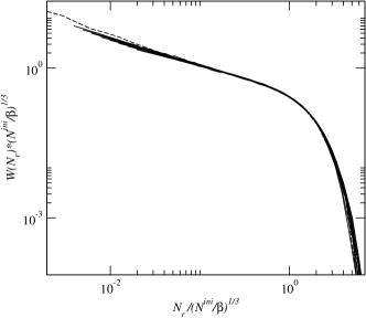
Figure 3: The function $W(N_{r})(N^{ini}/\beta)^{1/3}$ vs $N_{r}/(N^{ini}/\beta)^{2/3}$ for $\beta=0.5$ and $\beta=0.125$ and for $N^{ini}=2^{16},2^{17},2^{18},2^{19},2^{20},2^{21}$. The 12 curves converge with increasing $N$ towards an asymptotic curve, confirming the existence of an asymptotic scaling function $F(s)$. The dashed line shows the function $F(s)$ obtained using the data for $G(y)$ obtained from the same simulation and Eq. (18).

The number of nodes left in container $\mathcal{C}_{2}$ is $N_{c_{2}}=(\gamma/\beta)N_{r}$.

We thus have shown that the number of nonfrozen nodes scales with network size $N^{ini}$ as $(N^{ini})^{2/3}$, with most of these nodes receiving only one input from other nonfrozen nodes. The number of nonfrozen nodes receiving two inputs from nonfrozen nodes scales as $(N^{ini})^{1/3}$. We have found scaling functions that describe the probability distribution for these two types of nodes in the limit of large network size. Our next task will be to connect these nonfrozen nodes to a network. This is a reduced network, where all frozen nodes have been cut off.

5 Relevant nodes

Let us start from the result obtained from the stochastic process of the previous two sections. Each time we run this process we obtain $N$ nonfrozen nodes. Out of these, $N_{r}$ ($N_{c_{2}}$) nodes receive input from two other nonfrozen nodes and have a reversible (canalizing $\mathcal{C}_{2}$) update function. We define the parameter

$$a=\frac{N_{r}+N_{c_{2}}}{\sqrt{N}}=(1+\gamma/\beta)y^{3/2}\,,$$ (21)

which has a probability distribution $f(a)$ that is determined from the condition $f(a)da=G(y)dy$,

$$f(a)=\frac{2}{3a^{1/3}(1+\gamma/\beta)^{2/3}}G\left(\left(\frac{a}{1+\gamma/\beta}\right)^{2/3}\right)\,.$$ (22)

Just as $G(y)$, the function $f(a)$ is the exact probability distribution only in the thermodynamic limit $N^{ini}\to\infty$. We determine the relevant nodes by a stochastic process that removes iteratively nodes that are not relevant. Each of the $N$ nonfrozen nodes chooses its input(s) at random from the nonfrozen nodes. There are altogether $N(1+a/\sqrt{N})$ inputs to be chosen, and consequently the nonfrozen nodes have together $N(1+a/\sqrt{N})$ outputs. The number of outputs of a node is Poisson distributed with the mean value $(1+a/\sqrt{N})$. The fraction $\exp(-1-a/\sqrt{N})$ of nodes have no output. They are the leaves of the trees of the network of nonfrozen nodes, and we therefore know that they are not relevant. We put them in container number 1. Their number will change during the stochastic process that determines the relevant nodes. The other nodes are placed in container number 2. Their number is $N_{l}$ (“labelled”), and it will be reduced until only the relevant nodes are left. The total number of outputs of the nodes in container 2 is initially $N(1+a/\sqrt{N})$, while their total number of inputs is $N(1+a/\sqrt{N})(1-\exp(-1-a/\sqrt{N}))$. Now, we remove one node from container 1 and connect its input(s) at random to the outputs of the nodes in container 2. The chosen output(s) are cut off. If a node whose output is cut off has no other output left, we move the node from container 2 to container 1. It cannot be a relevant node since relevant nodes influence other relevant nodes. We iterate this procedure, until there is no node left in container 1. The nodes remaining in container 2 are the relevant nodes. During the entire process, the number of outputs in container 2 is identical to the number of inputs in container 1 and 2. As long as container 1 is not empty, there are more outputs in container 2 than inputs, and only when the process is finished do the two numbers become identical. We can therefore simplify the stochastic process by removing container 1 altogether. We simply have to continue cutting of outputs from nodes in container 2 and removing nodes with no outputs, until the total number of outputs of the nodes in container 2 has become identical to their total number of inputs. The remaining nodes are relevant, and we have then $N_{l}^{final}\equiv N_{rel}$. These nodes can then be connected to a network by connecting the inputs and outputs pairwise.

In order to derive analytical results, it is useful to run this process backwards. Starting with $N$ nodes with no outputs, adding outputs at random will eventually generate the Poisson distribution of the number of outputs per node that we have started with. The reverse stochastic process is therefore defined by the following rule: Begin with an empty container (former container 2) and $N$ nodes outside the container. Most of these nodes have one input, and the fraction $a/\sqrt{N}$ have two inputs. Add an output to a randomly chosen node. Put this node in the container. Add another output to a randomly chosen node (choosing every node with equal probability, whether the node is inside or outside the container). If a node from outside the container is chosen, put it in the container. Eventually, the total number of outputs in the container will become larger than the total number of inputs in the container. The container contains the relevant nodes at the moment when the inputs equal the outputs for the last time.

In order to show that the number of relevant nodes scales with $\sqrt{N}$, we define a scaling variable

$$t=\frac{N_{l}}{\sqrt{N}}\,.$$

During one step, an output is added to nodes that are already in the container with probability ${N_{l}}/N$. Let $N_{o}$ count the number of outputs that have been added to nodes in the container, i.e., $N_{o}=$(total number of outputs in the container) $-N_{l}$. Then the average rate of increase of $N_{o}$ is given for sufficiently large $N$ by

$$\langle\frac{dN_{o}}{dN_{l}}\rangle=\frac{N_{l}}{N}\,,$$

or

$$\langle\frac{dN_{o}}{dt}\rangle=t\,.$$

Let $N_{i}$ count the number of nodes in the container with two inputs. Their rate of increase is

$$\langle\frac{dN_{i}}{dN_{l}}\rangle=\frac{a}{\sqrt{N}}\,,$$

or

$$\langle\frac{dN_{i}}{dt}\rangle=a\,.$$

Consequently, the probability distribution for $N_{o}$ is given by

$$P_{o}(N_{o}|t)=\frac{1}{N_{o}!}e^{-t^{2}/2}\left(\frac{t^{2}}{2}\right)^{N_{o}}\,,$$ (23)

and the probability distribution for $N_{i}$ is given by

$$P_{i}(N_{i}|t)=\frac{1}{N_{i}!}e^{-at}\left(at\right)^{N_{i}}\,.$$ (24)

The stochastic process can be viewed as a random walk that steps to the right with a rate $t$ and to the left with a rate $a$. It is finished when $N_{i}=N_{o}$ for the last time, i.e. when the walk leaves the origin for the last time. We determined the probability distribution $\mathcal{C}_{a}(t)$ for this last exit time from the origin by a computer simulation. It is shown in Fig. 4 for $a=1$. For small $t$, it increases linearly in $t$, because the probability of making a step to the right is proportional to $t$ for small times.

Figure 4: The function $\mathcal{C}_{1}(t)$ as obtained by running the stochastic process described in this section. The dotted line corresponds to the function $0.25t$, which is a good fit to $\mathcal{C}_{1}(t)$ for small $t$.

For $a=0$, we can obtain an analytical result from the relation

$$\mathcal{C}_{0}(t)=-\frac{\partial P_{o}(0,t)}{\partial t}=te^{-t^{2}/2}\,.$$ (25)

Since we were able to write the stochastic process in terms of $t$ and $a$ alone, the probability distribution for the number of relevant nodes depends only on the combination $N_{rel}/{\sqrt{N}}$ and on the parameter $a$,

$$p_{a}(N_{rel})dN_{rel}=\mathcal{C}_{a}\left(N_{rel}/{\sqrt{N}}\right)dN_{rel}/{\sqrt{N}}\,.$$ (26)

The relation between $N$ and $a$ is obtained using Eq. (8) and (21):

$$\sqrt{N}=a^{1/3}\left(\frac{N^{ini}}{\beta+\gamma}\right)^{1/3}\,.$$

Taking into account the probability distribution (22) of the parameter $a$, we obtain the scaling behavior of the number of relevant nodes,

$$p(N_{rel})=\int_{0}^{\infty}daf(a)\mathcal{C}_{a}\left(\frac{N_{rel}a^{-1/3}}{(N^{ini}/(\beta+\gamma))^{1/3}}\right)\left(\frac{\beta+\gamma}{aN^{ini}}\right)^{1/3}\,.$$ (27)

The error made by taking the upper limit of the integral to infinity vanishes for $N^{ini}\to\infty$. We introduce the scaling variable

$$z=\frac{N_{rel}}{\left(\frac{N^{ini}}{\beta+\gamma}\right)^{1/3}}\,,$$ (28)

which has then the following probability distribution

$$P(z)=\int_{0}^{\infty}da\frac{f(a)}{a^{1/3}}\mathcal{C}_{a}\left(\frac{z}{a^{1/3}}\right)\,.$$ (29)

The probability distribution for the number of relevant nodes depends for large $N^{ini}$ only on the scaling variable $z$. We determined numerically the function $P(z)$ by combining the two stochastic processes described in this paper. First, we determined a value of $a$ using the process of Section 4. Then, we used this value of $a$ to determine the last exit time of the stochastic process of this section, giving a value of $z$. The shape of the curves $P(z)$ depends on the value of $\gamma/\beta$, and the results are shown in Fig. 5 for $\gamma/\beta=0$ and $\gamma/\beta=4$, which is the original Kauffman model, where each update function has the same weight. It is easy to check analytically that

$$\lim_{z\to 0}P(z)=\sqrt{2\pi}/4(1+\gamma/\beta)^{1/3}\,.$$

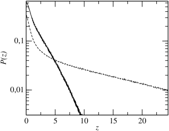
Figure 5: The function $P(z)$ for $\gamma/\beta=0$ (solid line) and $\gamma/\beta=4$ (dashed line). The results were obtained by running the two coupled stochastic processes for $10^{7}$ samples.

The mean number of relevant nodes is

$$\bar{N}_{rel}=\int_{0}^{\infty}N_{rel}p(N_{rel})dN_{rel}=\left(\frac{N^{ini}}{\beta+\gamma}\right)^{1/3}\int_{0}^{\infty}zP(z)dz\,,$$ (30)

i.e., it is proportional to $(N^{ini})^{1/3}$. Finally, let us give the probability distribution for the number of relevant nodes with two relevant inputs. Let $m$ denote the number of relevant nodes with two relevant inputs and $\tilde{P}(m;z)dz$ the probability of having the number of relevant nodes in the interval $[N_{rel}(z),N_{rel}(z+dz)]$, with $m$ of them having two relevant inputs. Using Equations (23) and (24), we can express $\tilde{P}$ as

$$\tilde{P}(m;z) = \int_{0}^{\infty}da\frac{f(a)}{a^{1/3}}\mathcal{C}_{a}\left(\frac{z}{a^{1/3}}\right)$$

$$\quad\times\frac{P_{o}\left(m|za^{-1/3}\right)P_{i}\left(m|za^{-1/3}\right)}{\sum_{l}P_{o}\left(l|za^{-1/3}\right)P_{i}\left(l|za^{-1/3}\right)}\,.$$

As $P_{o}$ and $P_{i}$ decay exponentially fast with increasing $m$, the mean number of relevant nodes with two inputs is finite.

6 Conclusions

In this paper, we have obtained the asymptotic probability distributions in the limit of large network size for the number of nonfrozen nodes, the number of nonfrozen nodes with two nonfrozen inputs, the number of relevant nodes, and the number of relevant nodes with two relevant inputs. The mean values of these quantities scale with network size $N^{ini}$ as a power law in $N^{ini}$, with the exponent being $2/3$, $1/3$, $1/3$, and $0$ respectively. The implications of the results are manifold.

First, the notion that these networks are “critical” is now corroborated by the existence of power laws and scaling functions. Originally, it was expected that the quantities that display the scaling behavior should be the attractors of the network Kauffman (1969). In the meantime, it has become clear that mean attractor numbers do not obey power laws Samuelsson and Troein (2003). It is the number of nonfrozen and relevant nodes that show scaling behavior.

Next, let us compare the results to those of critical $K=1$ networks. A $K=1$ critical network with $N$ nodes corresponds to the nonfrozen part of a critical $K=2$ network for $a=0$. In this case, the probability distribution of the number of relevant nodes is given by Eq. (26) with $a=0$,

$$p_{0}(N_{rel})=\frac{1}{\sqrt{N}}\mathcal{C}_{0}\left(\frac{N_{rel}}{\sqrt{N}}\right)=\frac{N_{rel}}{N}e^{-N_{rel}^{2}/2N}\,.$$ (32)

The mean number of relevant nodes is proportional to $\sqrt{N}$. When these relevant nodes are connected to a network by pairwise connecting the inputs and outputs, one obtains a set of simple loops. From Drossel et al. (2005), we know that there is a mean number of $\ln\sqrt{N}$ loops and that the number of loops of length $l$ in a critical $K=1$ network is Poisson distributed with a mean $1/l$ for $l\ll\sqrt{N}$. This can be easily explained by consindering the process of connecting inputs and outputs: We begin with a given node and draw the node that provides its input from all possible nodes. Then, we draw the node that provides the input to the newly chosen node, etc., until the first node is chosen and a loop is formed. For small loop size, the probability that the loop is closed after the addition of the $l$th node is $1/N_{rel}$. Therefore, the probability that a given node is on a loop of size $l$ is $1/N_{rel}$, and the mean number of nodes on loops of size $l$ is 1, and the number of loops of length $l$ is Poisson distributed with a mean $1/l$ for sufficiently small $l$.

Now, the $K=2$ critical networks have of the order of $(N^{ini})^{1/3}$ relevant nodes, with only a finite number of them having two relevant inputs. The relevant components are constructed from the relevant nodes by pairwise connecting inputs and outputs. In the asymptotic limit of very large $N^{ini}$ that we are considering, the probability that a randomly chosen relevant node has two inputs or two outputs vanishes. Let us again construct a component by starting with one node and choosing its input node etc., until the component is finished. If the component is small, it consists almost certainly only of nodes with one input and one output and is therefore a simple loop. There is no difference between the statistics of the small relevant components of a $K=1$ critical network, and the number of loops of length $l$ is Poisson distributed with a mean $1/l$. The total number of relevant nodes in loops of size $l\leq l_{c}$ with $l_{c}=\epsilon(N^{ini})^{1/3}$ (with a small $\epsilon$) is $l_{c}$, and it is a small proportion of all nodes. If there were no nodes with two inputs or outputs, the number of components larger than $l_{c}$ would be $(\ln N_{rel}-\ln l_{c})=\ln(1/\epsilon)$. The additional links may reduce this number, which is in any case finite. Since these large components contain almost all nodes, they contain almost all relevant nodes with two inputs or outputs.

From these findings, we can obtain results for the attractors of $K=2$ critical networks. The numbers and lengths of attractors are determined by the relevant components. We now argue that the mean number and length of attractors increases faster than any power law. If we remove the components of size larger than $l_{c}$ and determine the mean number and length of attractors for this reduced relevant network, we have a lower bound to the correct numbers. Now, the reduced relevant network of a $K=2$ system is identical to that of a critical $K=1$ system (where the critical loop size is $l_{c}=\epsilon\sqrt{N}$). In Drossel et al. (2005), it was proven that the mean number and length of attractors for such a reduced $K=1$ system increases faster than any power law with network size. We therefore conclude that the same is true for critical $K=2$ networks.

Earlier, Samuelsson and Troein Samuelsson and Troein (2003) have derived analytically an exact expression for the number of attractors of length $L$ of a critical $K=2$ network in the limit of large $N^{ini}$, and they have pointed out that this implies that the mean number of attractors increases faster than any power law with $N^{ini}$. Using their calculation, it has recently been shown Drossel (2005) that there is a close relationship between $K=1$ critical networks and the nonfrozen part of $K=2$ critical networks, and that the results of Samuelsson and Troein (2003) can be most naturally interpreted if the relevant components of these two networks look identical for component sizes below the above-given cutoffs. This interpretation is placed on a firm foundation by the present paper.

References

- Kauffman et al. (2003) S. Kauffman, C. Peterson, B. Samuelsson, and C. Troein, in Proceedings of the National Academy of Sciences USA (2003), no. 25 in 100, pp. 14796–14799.
- Kauffman (1969) S. A. Kauffman, J. Theor. Biol. 22, 437 (1969).
- Derrida and Pomeau (1986) B. Derrida and Y. Pomeau, Europhys. Lett. 1, 45 (1986).
- Derrida and Stauffer (1986) B. Derrida and D. Stauffer, Europhys. Lett. 2, 739 (1986).
- Aldana-Gonzalez et al. (2003) M. Aldana-Gonzalez, S. Coppersmith, and L. P. Kadanoff, Perspectives and Problems in Nonlinear Science pp. 23–89 (2003).
- Flyvbjerg (1988) H. Flyvbjerg, J. Phys. A 21, L955 (1988).
- Flyvbjerg and Kjær (1988) H. Flyvbjerg and N. J. Kjær, J. Phys. A 21, 1695 (1988).
- Bastolla and Parisi (1998a) U. Bastolla and G. Parisi, Physica D 115, 203 (1998a).
- Bastolla and Parisi (1998b) U. Bastolla and G. Parisi, Physica D 115, 219 (1998b).
- Socolar and Kauffman (2003) J. E. S. Socolar and S. A. Kauffman, Phys. Rev. Lett. 90, 068702 (2003).
- Samuelsson and Troein (2003) B. Samuelsson and C. Troein, Phys. Rev. Lett. 90, 098701 (2003).
- Drossel (2005) B. Drossel, Phys. Rev. E 72, xxx (2005).
- Drossel et al. (2005) B. Drossel, T. Mihaljev, and F. Greil, Phys. Rev. Lett. 94, 088701 (2005).