Spin and temperature dependent study of exchange and correlation in thick two-dimensional electron layers.

Abstract

The exchange and correlation $E_{xc}$ of strongly correlated electrons in 2D layers of finite width are studied as a function of the density parameter $r_{s}$, spin-polarization $\zeta$ and the temperature $T$. We explicitly treat strong-correlation effects via pair-distribution functions, and introduce an equivalent constant-density approximation (CDA) applicable to all the inhomogeneous densities encountered here. The width $w$ defined via the CDA provides a length scale defining the $z$-extension of the quasi-2D layer resident in the $x$-$y$ plane. The correlation energy $E_{c}$ of the quasi-2D system is presented as an interpolation between a 1D gas of electron-rods (for $w/r_{s}>1$) coupled via a log(r) interaction, and a 3D Coulomb fluid closely approximated from the known three-dimensional correlation energy when $w/r_{s}$ is small. Results for the $E_{xc}(r_{s},\zeta,T)$, the transition to a spin-polarized phase, the effective mass $m^{*}$, the Landé $g$-factor etc., are reported here.

I Introduction.

The 2D electron systems (2DES) present in GaAs or Si/SiO₂ structures access a wide range of electron densities, providing a wealth of experimental observationskrav . The 2D electrons reside in the x-y plane and also have a transverse ($z$-dependent) density $n(z)$ which is confined to the lowest subband of the hetero-structureafs . The 2D character arises since the higher subbands are sufficiently above the Fermi energy $E_{F}$. Then the physics depends only on the “coupling parameter” $\Gamma$ = (potential energy)/(kinetic energy), the $z$-distribution $n(z)$, the spin-polarization $\zeta$, and the temperature $T$ which has to be significantly smaller than the Fermi energy $E_{F}$ to preserve the 2-D character. The $\Gamma$ for the 2DES at the density $n$ is equal to the mean-disk radius $r_{s}=(\pi n)^{-1/2}$ per electron, expressed in effective atomic units which depend on the bandstructure mass $m_{b}$ and the “background” dielectric constant $\epsilon_{b}$. The $z$-motion in the lowest subband may have widths of $\sim 600$ Å, in GaAs when $r_{s}$ is $\sim 6$, in heterojunction insulated-gate field-effect transistors (HIGFET) which have been an object of recent studieszhu . Similarly, other nanostructures (e.g., quantum dots) contain electrons confined to a micro-region in the $x$-$y$ plane, and have a sizable $z$ extensionwilliams . Hence layer-thickness effects are important in many areas of nanostructure physics. Appropriate correlation functionalsmartin for such systems are still unavailable, even though the exchange functional for Fang-Howard distributions is known sternjjap .

Layer thickness effects are a long standing probe of exchange and correlation theories in 3D electron slabsperdew . The relevance of the finite size of the 2D layers had also been considered within the quantum Hall effectahm ; dassarmaqh , and more recently in the context of the $g$-factor and the effective mass $m^{*}$ of 2-D layertutuc ; tan ; morsen ; asgari ; zhang ; cdw . In the early days of the application of diagrammatic perturbation theory (PT) to condensed-matter problems, it was normal to attempt to calculate various many-body properties like the effective mass $m^{*}$, the effective $g$-factor $g^{*}$, and corrections to the total energy using perturbation methods. The need to go beyond the random-phase approximation (RPA) was rapidly appreciated and lead to the work of Hubbard, Rice, Vosko, Geldart and othersgeldart . The common experience with the generalized RPA method, when applied to 3D electrons and to ideally thin 2D layer is that it predicts a spin-polarized phase at unrealistic high densities (low $r_{s}$), while Quantum Monte Carlo (QMC) simulations suggest a density near $r_{s}\sim$ 25-26 in 2D. RPA methods lead to negative pair-distribution functions (PDFs), incorrect local-field corrections in the response functions, and disagreement with the compressibility sum rule and other formal conditions. Recent attempts to calculate the effective mass $m^{*}$ for ideally thin layersasgari ; zhang show strong disagreement with the $m^{*}$ obtained from QMC simulationskwon . In fact, the main thrust of the programs of Singwi, Tosi et al. (STLS)stls , and Ichimaru et al.ichimaru was to overcome the shortcomings of the RPA-like approach via non-perturbative methods. Many-body calculations where different parts of the calculation (e.g, vertex corrections, local-field corrections, etc.) are obtained from different sources, (e.g, vertex corrections from a model, local-field corrections or correlation energies from QMC, and some other quantities fitted to sum rules etc.) and combined together, have also appeared. Unless the same “mixture” is used to calculate a multitude of properties and shown to lead to consistent results, such theories have to be treated with caution.

We have introduced an approximate method for strongly correlated quantum systems where the objective is to work with the PDF of the quantum fluid, generated from an equivalent classical Coulomb fluid whose temperature $T_{q}$ is chosen to reproduce the correlation energy of the original quantum fluid at $T=0$. The classical PDFs are calculated via the hyper-netted-chain (HNC) equation, and the method is called the CHNC. As the method has been described in previous publicationsprl1 ; prb ; prl2 ; prl3 , and successfully applied to a variety of problemshyd ; 2valley ; locf ; eplmass , only a brief account is given here, mainly to help the reader. The PDFs are obtained from an integral equation which can be recast into a classical Kohn-Sham form where the correlation effects are captured as a sum of HNC diagrams and bridge diagrams.

$$g_{ij}(r)=\exp^{-\beta\left(P_{ij}(r)+V_{cou}(r)+N_{ij}(r)+B_{ij}(r)\right)}$$ (1)

The temperature of the classical fluid $T_{q}=1/\beta$ is chosen such that at $T=0$ the calculated classical $g(r)$ recovers the known correlation energy of the fully spin-polarized 2D electron fluid at the given density. This fitting has been done in ref. prl2 , and $T_{q}$ is known as a function of $r_{s}$. At finite-$T$, the classical fluid temperature $T_{cf}$ is taken to be

$$T_{cf}=(T^{2}_{q}+T^{2})^{1/2}$$ (2)

This $T_{cf}$ is used for all spin polarizations. In Eq. 1 the indices $i,j$ label the spin states. The $P_{ij}(r)$ is chosen to ensure that $g_{ij}(r)$ reduces to the explicitly known non-interacting PDF, $g_{ij}^{0}(r)$, when the Coulomb interaction $V_{cou}(r)$ is switched off. Thus $P_{ij}(r)$ takes care of Pauli-exclusion effects and ensures that the “Fermi-hole” is exactly recoveredlado . Also, $N_{ij}(r)$ is a sum of terms that appear in the hyper-netted-chain equation, while $B_{ij}(r)$ contains 3-body and higher-order diagrams not contained in the nodal term $N_{ij}(r)$. The latter depends implicitly on $g_{ij}(r)$, and is evaluated via the Ornstein-Zernike equation. The bridge term is very difficult to evaluate, but the hard-sphere fluid provides a good approximation. That is, in 2D, we specify $B_{ij}(r)$ by specifying the hard-disk radius $r_{H}$, or equivalently the packing fraction $\eta$, and use the Percus-Yevik approachharddisk . As the parallel-spin three-body clusters are suppressed by the Pauli exclusion, we use only a single bridge function, viz., $B_{12}(r)$. This makes the bridge interaction effectively independent of $\zeta$. Bulutay and Tanatar, and also Khanh and Totsujibuluty , have examined variants of CHNC without a bridge function (this is some what equivalent to neglecting back-flow terms in QMC simulations of 2D systems). The hard-sphere radius $r_{H}$, and the packing fraction $\eta$ are given byprl2 :

$$r_{H} = 2r_{s}\eta^{1/2}$$ (3)

$$\eta = 0.1175r_{s}^{1/3}(t_{cf}+t^{2}/2)$$ (4)

$$t_{cf} = T_{cf}/E_{F},\;\;\;t=T/E_{F}$$ (5)

A plot of the bridge function for a few typical cases is given in Fig. 1.

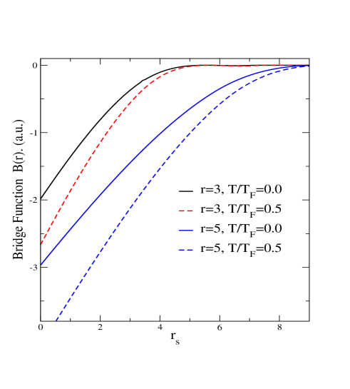
Figure 1: The bridge function $B(r)$ for $r_{s}=3$ and $r_{s}=5$. The effect of changing the temperature is also shown.

The CHNC method was applied to the 3D and 2D electron fluidsprl1 ; prb ; prl2 ; prl3 , to dense hydrogen fluidhyd , and also to the two-valley system in Si/SiO₂ 2DES2valley ; eplmass . In each case we showed that the PDFs, energies and other properties obtained from CHNC were in excellent agreement with comparable QMC results. The advantage of the CHNC method is that it affords a simple, semi-analytic theory for strongly correlated systems where QMC becomes prohibitive or technically impossible to carry out. The classical-fluid model allows for physically motivated treatments of complex issues like three-body clustering etc., which are difficult within quantum methods. The disadvantage, typical of such many-body approaches, is that at present it remains an “extrapolation” taking off from the results of a model fluid. The fully spin-polarized infinitely-thin uniform 2DES is the model fluidprl2 , as the $E_{c}$ of this one-component system is accurately known.

In this study we use a method of replacing the inhomogeneous electron distribution $n(\vec{r},z)=n(\vec{r})n(z)$ by a homogeneous density systemggsavin ; cdw i.e., a constant-density approximation (CDA) where the transverse density $n(z)$ is a constant within a slab of width $w$, and zero outside. The CDA avoids difficulties associated with gradient expansions noted in ref.martin . Also, the CDA presents a unified approach to quasi-2D distributions like the Fang-Howard modelafs , the quantum-well model etc. $E_{xc}$ for such distributions is calculated as a function of the spin polarization $\zeta$, 2-D density parameter $r_{s}$, the CDA width $w$ and the temperature $T$. This enables us to determine physical quantities related to the Landau Fermi liquid parameters. Thus the spin susceptibility enhancement, the effective mass $m^{*}$, and the Landé $g$ factor for the quasi 2D electrons are presented.

II The quasi-2D interaction

The transverse distribution $n(z)$ of the 2D electrons is given by the square of the lowest subband wavefunction $\phi(z)$ of the heterostructure, calculated within the envelope approximation. The nature of the materials used (e.g, Si/SiO₂ or GaAs) and the doping profiles determine the confining potential and the electron density $n(z)$ in the z-direction. Typically, $n(z)$ may be modeled by one of the following forms.

$$n(z) = \delta(z),\;\;\;\mbox{ideal thin layer}$$ (6)

$$= (2/w)\sin^{2}(\pi z/w),\;\;\;\mbox{infinite well}$$ (7)

$$= (b^{3}/2)z^{2}\exp(-bz),\;\;\;\mbox{Fang-Howard}$$ (8)

$$= 1/w,\;\;|z|\leq w\;\;\;\mbox{constant-density model}$$ (9)

The second and third are frequently used approximate (but adequate) models, while we present the fourth model, the CDM. This is an excellent constant-density approximation (to be called the constant-density approximation, CDA) to generate the effective 2-D potential arising from most $n(z)$ distributions, on suitably choosing $w$. The Fang-Howard (FH) formafs ; fangh , contains the parameter $b$, and is normalized in the range $0$ to $\infty$. The FH parameter $b$ is such that $b^{3}=(48*\pi/a_{0})(n_{d}+11n_{s}/32)$, where $n_{s}$ is the 2D electron density $n$, and $n_{d}$ is the depletion charge densityafs . The material parameters are contained in the effective Bohr radius $a_{0}=\epsilon_{b}\hbar^{2}/m_{b}e^{2}$ defined in terms of the usual constants, $\epsilon_{b}$ and $m_{b}$ being the dielectric constant and the band mass. For the devices used in ref. tan ; zhu , the depletion density has been reported to be negligiblemorsen . Then $b^{3}=33/(2r_{s}^{2})$, in atomic units.

II.1 The constant-density model.

We denote the Coulomb potential in an infinitely thin layer by $V(r)=1/r$, while $W(r)$ is used for the effective 2-D potential of a thick layer. The effective 2D-Coulomb potential $W(r)$ between two electrons having coordinates ($\vec{r_{1}},z_{1}$) and ($\vec{r_{2}},z_{2}$), with $\vec{r}=\vec{r_{1}}-\vec{r_{2}}$ is given by,

$$W(r)=\int_{0}^{z_{m}}\int_{0}^{z_{m}}\frac{dz_{1}dz_{2}n(z_{1})n(z_{2})}{[r^{2}+(z_{1}-z_{2})^{2}]^{1/2}}\\$$ (10)

Here $z_{m}$ is $\infty$ for FH, while $z_{m}=w$ for the others. The potential $W(r)=(1/r)F(r)$ and the form factor $F(r)$ reflects the effect of the $z$-extension of the density. There is no analytic form for $F(r)$ in the Fang-Howard case, while the $q$-space form, $F(q)$ is knownafs . If the dielectric constants of the barrier and well material were assumed equal, then the Fang-Howard form factor is:

$$F(q)=[1+\frac{9q}{8b}+\frac{3q^{2}}{8b^{2}}][1+\frac{q}{b}]^{-2}$$ (11)

Here we derive a potential $W(r,w)$ for the constant-density model(CDM) which is, to an excellent approximation electrostatically equivalent to the the 2D potential for any reasonable $n(z)$. These FH-type distributions are themselves convenient fits to the self-consistent Schrodinger solutions and have uncertainties of a few percent. The CDA holds well within such limits. The potentials are explicitly shown in Fig. 2 for the FH form where we have taken an extreme example with $b=0.1$. The method of replacing an inhomogeneous distribution by a uniform distribution is suggested by the observation that the non-interacting total pair-correlation function $h^{0}(r)$ has the form $\sim n(r)^{2}$, where $n(r)$ is the density -profile around the Fermi hole. In our case we wish to replace the inhomogeneous $n(z)$ by a constant-density distribution $n_{cd}$ which has the same electrostatic potential in the 2-D plane as $n(z)$.

$$n_{cd}=1/w=\int n(z)^{2}dz$$ (12)

Since the subband distribution is normalized to unity, the width $w$ of the constant-density slab is simply $1/n_{cd}$. Starting from different objectives, Gori-Giorgi et al.ggsavin have already proposed this formula for determining an average density for an inhomogeneous density, in the context of pair-distributions in 2-electron atoms. We have also shown the utility of the CDA in estimating the correlation energy of the 2DES in the Wigner-crystal phasejost . The $w$ of the CDA is somewhat different from the “thickness” $3/b$ often assigned to the FH distribution. In fact, the constant-density slab width $w$ for the Fang-Howard $b$ is given by $w=16/(3b)$.

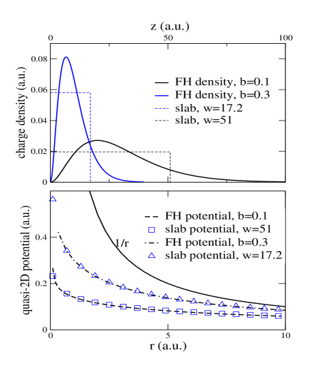
Figure 2: (a)The Fang-Howard density and the equivalent constant-density slab. (b)Comparison of the $1/r$ form with the quasi-2D potential from the Fang-Howard distribution for the FH parameter $b$ = 0.1, and 0.3 and the equivalent slabs at $w$ = 53.3 and 17.8 a.u. respectively.

The quasi-2D potential for a CDM of width $w$ is given by

$$W(r) = V(r)F(s),\;\;s=r/w,\;\;t=\surd{(1+s^{2})}$$ (13)

$$F(s) = 2s\left[\log\frac{1-t}{s}\,\,+1-t\right]$$ (14)

This potential tends to $1/r$ for large $r$, and behaves as

$$\frac{2}{w}\left(\ln\frac{2w}{r}+\frac{r}{w}-1\right)$$

for $r<w$. Thus the short-range behaviour is logarithmic and weaker than the Coulomb potential. The $k$-space form of the CDM potential is:

$$V_{usm}(k,w) = V(k)F(p),\,\,\,p=kw$$ (15)

$$F(p) = (2/p)\{(e^{-p}-1)/p+1\}$$ (16)

The form factors $F(s)$ and $F(p)$ tend to unity as $w\to 0$. These $r$-space and $k$-space analytic forms of the CDM lead to analytic formulae for the FH form. In our work we assume that a given distribution has been replaced by an equivalent uniform-slab distribution, and only the final $W(r)$ potential enters into the exchange-correlation calculations (the numerical work has been checked via direct calculations as well). In the case of GaAs-HIGFETS, if $n_{d}$ could be neglected, the $r_{s}$ parameter specifies the $b$ parameter and hence the width $w$ of the CDM. Then $b\sim r_{s}^{-2/3}$ and $w=2.09494r_{s}^{2/3}$.

III Exchange Free Energy for quasi-2D layers.

The exact exchange free energy $F_{x}$ for 2D layers of finite thickness can be readily evaluated using the quasi-2D potential $W(r)$ and the noninteracting pair-distribution functions $g^{0}_{ij}(r)$ of the 2-D fluid. Only the parallel-spin case $i=j$ is relevant. Also, $g^{0}_{ij}(r)$ for a slab of finite thickness is identical to that for an ideally thin 2D layer, both at $T=0$ and at finite-$T$. In fact, we find that the $T$ dependence of the $F_{x}$ of layers of finite thickness is very close to that of the ideally thin case.

III.1 Ideally-thin layer

The first-order unscreened exchange free energy $F_{x}$ consists of $F_{x}^{i}$, where $i$ denotes the two spin species. At $T=0$ these reduce to the exchange energies:

$$E_{i}^{x}/n=\frac{8}{3\surd{\pi}}n_{i}^{1/2}$$ (17)

Here $n_{1}=n(1+\zeta)/2$, and $n_{2}=n(1-\zeta)/2$. Then the exchange energy per particle at $T=0$, i.e., the total $E_{x}/n$ becomes

$$E_{x}/n=(E_{1}^{x}+E_{2}^{x})/n=-\frac{8}{3\pi r_{s}}[c_{1}^{3/2}+c_{2}^{3/2}]$$ (18)

where $c_{1}$ and $c_{2}$ are the fractional compositions $(1\pm\zeta)/2$ of the two spin species.

We define a reduced temperature $t=T/E_{F}$, $E_{F}=\pi n$, and the species-dependent reduced chemical potentials $\mu^{0}_{i}/T$ by $\eta_{i}$, reduced temperatures $t_{1}=t/(1+\zeta)$ and $t_{2}=t/(1-\zeta)$, based on the two Fermi energies $E_{F1}$ and $E_{F2}$ which are $E_{F}(1\pm\zeta)$. Then we have:

$$F_{i}^{x}/E_{i}^{x}=\frac{3}{16}t_{i}^{3/2}\int_{-\infty}^{\eta_{i}}\frac{I^{2}_{-1/2}(u)du}{(\eta_{i}-u)^{1/2}}$$ (19)

The $I_{-1/2}$ is the Fermi integral defined as usual:

$$I_{\nu}(z)=\int_{0}^{\infty}\frac{dxx^{\nu}}{1+e^{x-z}}$$ (20)

The $\eta_{i}$ are given by

$$\eta_{i}=\log(e^{1/t_{i}}-1)$$ (21)

In the paramagnetic case Eq. 19 reduces to the result given by Isihara et al. (see their Eq.3.4; they use a different definition of the Fermi integral). For small values of $t$, the exchange energy is of the form,

$$E_{x}(r_{s},t)=E_{x}(r_{s},0)[1+(\pi^{2}/16)t^{2}\log(t)-0.56736t^{2}+...]$$ (22)

The total exchange free energy is $F_{x}=\Sigma F_{i}^{x}$. The accurate numerical evaluation of Eq. 19 requires the removal of the square-root singularity by adding and subtracting, e.g, $I^{2}(-|\eta|)/(v-|\eta|)^{1/2}$ for the case where $\eta$ is negative, and $v=u$, and so on.

A real-space formulation of $F_{x}$ = $F_{1}^{x}+F_{2}^{x}$ using the zeroth-order PDFs fits naturally with the approach of our study. Thus

$$F_{x}/n=n\int\frac{2\pi rdr}{r}\sum_{i<j}h^{0}_{ij}(r)$$ (23)

Here $h^{0}_{ij}(r)=g^{0}_{ij}(r)-1$. In the non-interacting system at temperature $T$, the antiparallel $h^{0}_{12}$, viz., $g_{12}^{0}(r,T)-1$, is zero while

$$h_{11}^{0}({\bf r})=-\frac{1}{n_{i}^{2}}\Sigma_{{\bf k}_{1},{\bf k}_{2}}n(k_{1})n(k_{2})e^{i({\bf k}_{1}-{\bf k}_{2}){\bf\cdot}{\bf r}}\,\,=\,-[f(r)]^{2}$$

Here k, r are 2-D vectors and $n(k)$ is the Fermi occupation number at the temperature $T$. At $T=0$ $f(r)=2J_{1}(k_{i}r)/k_{r}$ where $J_{1}(x)$ is a Bessel function. As a numerical check, we have evaluated the exchange free energy by both methods, i.e., via k-space and r-space formulations.

We present a convenient analytic fit to the exchange free energy which is a universal function $F_{x}(t)/E_{x}$, for arbitrary $\zeta$. That is, the same function applies to any component, on using the reduced Fermi temperature of the spin species. The total $F_{x}$ is obtained by adding both spin contributions. The analytic fit is:

$$F_{i}^{x}(t,\zeta)/E_{i}^{x}(\zeta)=$$

$$\frac{1+C_{1}t_{i}+C_{2}t_{i}^{2}}{1+C_{3}t_{i}+C_{4}t_{i}^{2}}\,\tanh(1/\surd{t_{i}})$$

The fit coefficients $C_{i}$ are 3.27603, 4.81484, 3.33100, 6.51436. The temperature $t_{i}$ is $t/(1\pm\zeta)$, appropriate to the spin polarization. The exchange effects in the 2DES decay more slowly with temperature than in the 3D case where a tanh$(1/t)$ factor appears in Eq. 3.2 of ref. pdw84, . The above form does not explicitly contain the low-temperature logarithmic term, but it reproduces the value of 0.99382 at $t=0.05$, while the numerical integration gives 0.9939497. Similarly, at $t=1$, 10 and 30 the fit (integral) returns 0.63839 (0.63839), 0.22999 (0.22990), and 0.13421 (0.13410) respectively.

III.2 Thick 2-D layers.

The $T=0$ exchange energy is modified by the layer thickness $w$. The expression for $g^{0}_{ij}(r)$ depends only on $x=r/r_{s}$. Similarly, the quasi-potential $W(r)$ depends on the reduced variable $s=r/w$. Hence the exchange energy of the quasi-2D layer depends only on the ratio $w_{s}=w/r_{s}$. The exchange energy per electron at a density $n$, given by $r_{s}$, polarization $\zeta$, in a layer of width $w$ is given by:

$$Ei_{x}(r_{s},\zeta,w)=\frac{1}{2}nr_{s}\int_{0}^{\infty}2\pi dxh^{0}(x,\zeta)F(x/w_{s})$$ (25)

Even though we have analytic forms for $W(r)$ and $h^{0}(r)$ as well as their Fourier transforms, we have not found a convenient analytic result for the exchange energy at $T=0$. However, the results can be parametrized by simple analytic-fit formulae:

$$E_{x}(r_{s},\zeta,w) = E_{x}(r_{s},\zeta,0)Q(w_{s},\zeta),\,\,w_{s}=w/r_{s}$$

$$Q(w_{s},\zeta) = \frac{1+A(\zeta)\surd{w_{s}}}{1+B(\zeta)\surd{w_{s}}+C(\zeta)w_{s}}$$

Here $E_{x}(r_{s},\zeta,0)$ is the exchange energy of the ideally thin system given by eq. 18. The ratio $Q(w_{s},\zeta)$ is a measure of the reduction in the exchange energy due to the thickness effect. Since the effect depends on $w_{s}=w/r_{s}$, for a given thickness, the effect is greater for high density samples. If the depletion density $n_{d}$ in HIGFETS could be neglected, and if the exchange-correlation energy $E_{xc}$ is not included in the energy minimization which determines the Fang-Howard parameter $b$, then $w_{s}\sim 2.09r_{s}^{-1/3}$. The inclusion of $E_{xc}$ in self-consistently determining $b$ changes $b$ by $\sim 2\%$ for low $r_{s}$, but the effect becomes less important at higher $r_{s}$. At $r_{s}$=1, and 10 for $\zeta=0$, the ratio $Q$ is 0.652 and 0.794 respectively. The reduction from the ideally-thin 2D form is clearly substantial. The exchange free energy $F_{x}(r_{s},\zeta,T,w)$ at finite-$T$, for layers with thickness $w$ is found to be adequately approximated by the temperature factor of the ideally-thin system. However, in calculating the effective mass from the finite-$T$ energies, we make independent calculations near $T=0$ and d͡o not use the fit given here.

Table 1: Parameters fitting the exchange energy ratio as a function of the layer width ratio $w_{s}=w/r_{s}$.

$\zeta$	$A$	$B$	$C$
0.0	0.155294	0.142486	0.320735
0.5	0.184536	0.169822	0.370001
1.0	0.19838	0.179455	0.462789

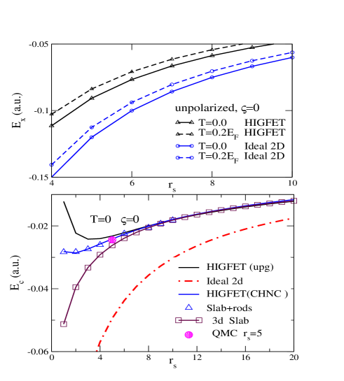
Figure 3: (a)The exchange energy $E_{x}$ (Hartree a.u.) of a 2DES in a HIGFET compared to that of an ideal 2DES, at $T/E_{F}=0$ and 0.2, with $\zeta=0$. (b)The correlation energy $E_{c}$ at $T=0$ and $\zeta=0$, for the HIGFET layer. HIGFET(upg) is the “unperturbed-$g$” approximation. HIGFET(CHNC) is the full calculation. This is compared with the correlation energy of a 3d slab model, and the “slab+rod”model. The QMC datum for a HIGFET ar $r_{s}=5$ is from De Palo et aldepalo .

The exchange energy for a HIGFET with $n_{d}=0$ is shown in Fig. 3 as a function of $r_{s}$ for $\zeta=0$ and temperature $T/E_{F}$=0 and 0.2.

IV The exchange-correlation energy for quasi-2D layers.

The correlation function $h^{0}(r)$ yields exact exchange energies for arbitrary layer thicknesses. In contrast, the correlation energies require a coupling-constant integration over the pair functions $g(r,\zeta,w,\lambda)$ calculated using the quasi-2D potential $\lambda W(r)$ for each $\lambda$. These $g(r,\zeta,w)$ can be calculated using the CHNC. On the other hand, the unperturbed-$g$ approximation, found to be useful in Quantum Hall effect studiesahm , has been exploited by De Palo et al.morsen . They have used the pair functions $g(r,\zeta,w=0)$ of the ideally thin layer obtained form QMC to calculate a correction energy $\Delta$ given by,

$$\Delta E=(n/2)\int 2\pi rdr[W(r)-V(r)]h(r,\zeta,w=0)$$ (26)

Then the total exchange-correlation energy $E_{xc}(r_{s},\zeta,w)$ is obtained by adding to $\Delta$ the known $E_{xc}$ of the ideally-thin system. The above equation can also be applied at finite temperatures using the finite-$T$ pair functions $g(r_{s},\zeta,T)$ obtainable from the CHNC procedure.

De Palo et almorsen have performed Diffusion-Monte-Carlo simulations at $r_{s}$ =5 for HIGFETS with $b=0.8707$, i.e, a CDM width $w$=6.1256 a.u., and find that the error in this approach compared to the full simulation is about 2%. This full QMC result at $r_{s}=5$ is shown in the lower panel of Fig. 3. Since the HIGFET system approximates to a thin-layer as $r_{s}$ increases, this approach is probably satisfactory for $r_{s}\geq$ 5. The method becomes unreliable for small $r_{s}$, and definitely fails below $r_{s}=2$. Also, the “unperturbed-$g$” approximation fails to include the renormalization of the kinetic energy picked up via the coupling constant integration over the fully consistent $g(r,w)$. We report results(Fig. 3) from the full coupling-constant integration of the $g(r,w)$, (Fig. 3, lower panel, CHNC) as well as from the “unperturbed-$g$” approximationmorsen used by De Palo et al.

In parametrizing the quasi-2D correlation energy $E_{c}(r_{s},w)$, we present an intuitive model of $E_{c}(r_{s},w)$. For small $r_{s}$, the ratio $w/r_{s}$ is large and the electrons are like 1-D wires with the axis normal to the 2D plane and interacting with a $\log(w/r)$ interaction (c.f., Eq. 13). However, at large $r_{s}$ we have 3-D like electron disks with $w$ and $r_{s}$ of comparable magnitude in the density regimes of interest in HIGFETS. Thus we model the quasi-2D $E_{c}$ as an interpolation between a 1D like form and a 3D like form. First we consider a purely 3D model. Given the 2D-density $r_{s}$ and an effective CDM width $w$, we define an effective 3D density parameter $r_{s}^{3d}$, purely for calculating its correlation energy. It will be seen that this 3D model is excellent for $r_{s}>7$. When $r_{s}$ becomes small (i.e, less than $\sim 3$), the effective width of the 2D layer, viz., $w/r_{s}$ becomes large and a 1D log-interaction modelsamaj is needed. To capture the rod-like regime, we define the “rod like” correction $\Delta E_{c}$ for $r_{s}<7$ by:

$$\Delta E_{c}(\zeta=0)=a_{0}+a_{L}\log(1/r_{s})+a_{1}r_{s}$$ (27)

where, for HIGFETS, $a_{L}=0.0221788$, $a_{1}=0.00365169$, and $a_{0}=0.0192979$ for $\zeta=0$. This $\Delta E_{c}$ is added to the 3-D slab form given below. The fit parameters for the $\zeta=1$ “rod-like” correction are $a_{0}$=0.013337, $a_{L}$=0.0084787, and $a_{1}$=0.0006821, to be applied for $r_{s}<15$.

For the 3D slab-like regime (i.e, $r_{s}>7$ for $\zeta$=0, $r_{s}>15$ for $\zeta=1$) we define a $\zeta$-dependent 3-D density parameter and a correlation energy via:

$$E_{c}(r_{s},\zeta,w) = E^{3d}_{c}(r_{s}^{3d},\zeta)$$ (28)

$$R_{s} = r_{s}/F(r_{s})$$ (29)

$$r_{s}^{3d} = [wR_{s}^{2}]^{1/3}Z(\zeta)$$ (30)

$$Z(\zeta) = \frac{2\surd{2}}{(4-\zeta)^{1/2}}(c_{1}^{1.5}+c_{2}^{1.5})$$ (31)

The 3D correlation energy $E^{3d}_{c}(r_{s}^{3d},\zeta)$ is that given by, e.g., Ceperley and Aldercepalder , or Gori-Giorgi and Perdewg-gp . We see from the lower panel of Fig. 3 that the correlation energy for small $r_{s}$, calculated using the 3D slab begins to go below the “unperturbed-g” approximation of Eq. 26, consistent with the trend of the ideal 2D gas, and the trend of the only QMC data point available for a HIGFET, at $r_{s}=5$. The exchange-correlation energy obtained from the full CHNC calculation is in excellent agreement with the QMC datum. The curve labeled ”Slab+rods” in Fig. 3 is the combined formula, Eq. 27, and Eq. 28, for the correlation energy/electron, with, for example, the region $r_{s}\sim 7$ for $\zeta=0$ obtained by linear interpolation between $r_{s}$=6 and $r_{s}=8$. This is clearly seen to reproduce the full CHNC results very well.

IV.1 Correlation energy at finite temperatures.

The correlation contribution to the Helmholtz free energy of the ideal 2-D layer, and layers of thickness $w$ can be easily calculated using the approach of Eq. 26, where the CHNC-generated finite-$T$ pair functions are used. A typical set of results at very low temperatures is given in Table 2. Here we have also given the packing fraction $\eta$ of the hard-sphere bridge function used to mimic the three-body and multi-body correlation contributions. As discussed in earlier workeplmass , the $F_{x}$ and the $F_{c}$ at very low $T$ contain logarithmic terms which cancel with each other, so that the sum $F_{xc}=F_{x}+F_{c}$ is free of such terms. From our numerical work we find that the $T$ dependence of the $F_{x}$ and $F_{c}$ of layers of finite thickness is very similar to that of ideally thin layers. Hence we assume that the logarithmic corrections are also similar. At $r_{s}=5$ the cancellation is good to about 75%, and this improves as $r_{s}$ increases. Although the two-component fluid (up spins and down spins) involves three distribution functions, we have, as beforeprl2 , used only one hard-disk bridge function, $B_{12}$, as clustering effects in $g_{ii}$ are suppressed by the Pauli-exclusion. However, at high densities (low $r_{s}$), the use of three bridge functions seems to be needed for satisfying various subtle features that are needed to ensure the exact cancellation of logarithmic energy terms etc. Instead of introducing additional features into the CHNC method, we have however retained the single bridge-function model that was used by us so farprl2 .

Table 2: Low-temperature data for the exchange-correlation contribution to the Helmholtz free energy, $F_{xc}$ per electron in atomic units at $r_{s}=5$, for the ideal 2D system and for a CDM of width 6.1256 au., i.e., Fang-Howard $b$=0.8707. The packing fractioin $\eta$ which defines the hard-disk bridge function is also given

$t=T/E_{F}$	$\eta$	$F_{xc}$(ideal)	$F_{xc}(Eq.~{}\ref{unpertg})$	$F_{xc}$(CHNC)
0.05	0.3718	-0.16902	-0.11197	-0.11467
0.08	0.3725	-0.16883	-0.11177	-0.11448
0.10	0.3730	-0.16867	-0.11161	-0.11433
0.12	0.3733	-0.16850	-0.11144	-0.11417

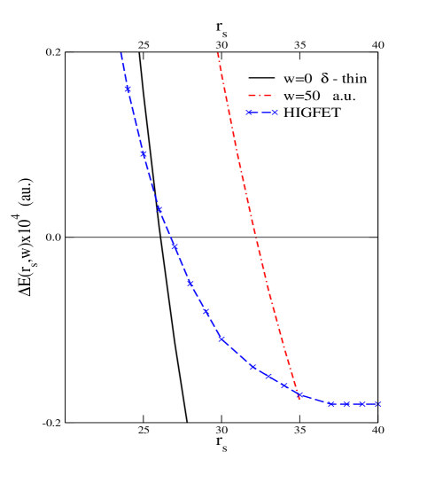
Figure 4: The Energy difference between the fully polarized and unpolarized states of 2D layers with different CDM widths $w$. The HIGFET $w$ varies as $r_{s}^{2/3}$ and is $\sim$ 18 near the spin-phase transition.

IV.2 The transition to a spin-polarized phase.

QMC simulations as well as CHNC calculations show that there is a spin-polarization transition (SPT) in the ideally-thin 2D electron fluid near $r_{s}\sim 26$. On the other hand, the correlation contributions dominate over the exchange energy in the 2-valley 2D system in Si MOSFETS, and the SPT is suppressed2valley . The rapid increase in $m^{*}$, with $g^{*}$ remaining unchanged while $r_{s}$ is increased, observed by Shashkin et al.shash was found to be consistent with this pictureeplmass . In finite-thickness 2D layers, as the CDM width $w$ increases, the location of the SPT is pushed to higher values, as seen in Fig. 4. In the case of HIGFETS used by, e.g., Tan et al.tan , the width $w$ increases with $r_{s}$, but only as $r_{s}^{2/3}$. Thus at $r_{s}$=26, the $w$ is only 18.4, and the SPT remains intact and occurs at a somewhat higher $r_{s}$, as shown by de Palo et almorsen , and also in Fig. 4. A natural consequence of delaying the SPT is to decrease the spin-susceptibility enhancement. The effective thickness of the quasi-2D layer can be increased by suitably designing the shape of the potential well, or including an additional subband, and in this case the SPT can be circumvented. However, a discussion of higher subband effects is outside the scope of this study.

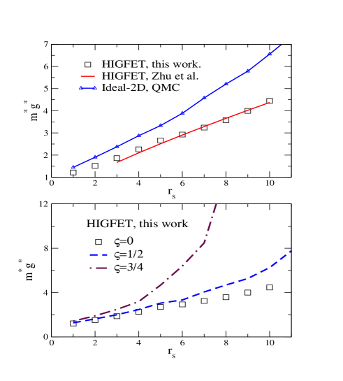
Figure 5: (a)The spin-susceptibility enhancement, i.e., $\chi_{s}/\chi_{P}$=$m^{*}g^{*}$ as a function of $r_{s}$ for the HIGFET. The experimental data of Zhu et al.zhu are also shown. (b)Variation of $m^{*}g^{*}$ as a function of the spin-polarization for a HIGFET.

V The spin-susceptibility, effective mass and the $g$-factor

The results for the exchange-correlation free energy $F_{xc}(rs,\zeta,T)$ for the ideal 2D system and the thick-layer system contain all the information needed to calculate the spin-susceptibility enhancement, the effective mass $m^{*}$ and the effective Landé factor $g^{*}$, for the ideal system and the thick layer. In fact, the following quantities are calculated from the respective second derivatives of the energy.

$$m^{*} = C_{v}/C_{v}^{0}=1+\frac{\left[\partial^{2}F_{xc}(t)/\partial t^{2}\right]}{\left[\partial^{2}F_{0}(t)/\partial t^{2}\right]}$$ (32)

$$\chi_{P}/\chi_{s} = (m^{*}g^{*})^{-1}=1+\frac{\left[\partial^{2}F_{xc}(\zeta)/\partial\zeta^{2}\right]}{\left[\partial^{2}F_{0}(\zeta)/\partial\zeta^{2}\right]}$$ (33)

We use the available QMC results for the ideal 2D exchange-correlation energy at $T=0$, and where convenient, the QMC pair-distribution functions at $T=0$ as parametrized by Giri-Giorgi et alggpair . The CHNC is used to obtain the pair-functions for situations (e.g, at finite-$T$ and finite thickness) where the QMC data are simply not available or difficult to use. In most cases, replacing the QMC-PDFs with the CHNC ones, or using the “unperturbed-$g$” approximation leads to relatively small changes. The exception is in the calculation of $m^{*}$, where the “unperturbed-$g$” approximation, Eq. 26, is inadequate.

V.1 The effective mass $m^{*}$.

In Fig. 6 we present our results for the ideal-2DES. No experimental results are available for this case, but limited QMC simulationskwon as well as results from diagrammatic perturbation theory (PT) asgari ; zhang are available.

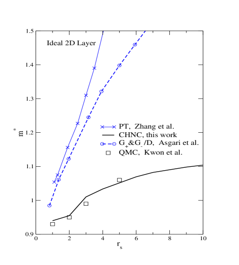
Figure 6: The effective mass $m^{*}$ of an ideal 2D layer ($w=0$) obtained from CHNC are compared with the the Quantum Monte Carlo data of Ref. kwon and the perturbation theory calculations of Zhang et al.zhang , and Asgari et al.asgari , i.e., their $G_{+}\&G_{-}/D$ calculation.

The CHNC based $m^{*}$ values have an error of at most $\pm$ 2%. The ideal 2D-layer $m^{*}$ shows a rapid rise around $r_{s}$=2 to 5, in good agreement with the four values from QMC, and then slows down in strong contrast to the $m^{*}$ proposed by Asgari et al., and Zhang et al. We have displayed the model denoted $G_{+}\&G_{-}/D$ by Asgari et al., as being their optimal choice from among the many models given in Ref. asgari , where they also contest the analysis of Zhang et al. The PT approaches are partly semi-phenomenological in that QMC data are input into local-field factors and other ingredients of the calculation; the choice of the vertex functions, treatment of on-shell or off-shell effects, whether to use self-consistent propagators or not, etc., are components of the prescription used by different workers. The strong disagreement of the PT-based $m^{*}$ with the QMC-based $m^{*}$ is notable.

The CHNC method has some similar uncertainties, especially in the use of a Percus-Yevik hard-sphere bridge function $B(r)$ to capture the back-flow like three-body contributions to the PDFs and the total energy. As seen in Fig. 1, the $T$ dependence of $B(r)$ seems quite small, and our initial calculations of $m^{*}$, reported in Ref. ssc were based on the zero-$T$ form of $B(r)$. This leads to an $m^{*}$ which drops slightly below unity and remains there. In this calculation we have used the proper $T$-dependent bridge function and the calculated $m^{*}$ is in good agreement with the QMC-based $m^{*}$. This might be somewhat coincidental, as the QMC results are also based on sensitive approximations. However, it means that we do have a $B(r)$ which is consistent with current QMC results, and hence may be used with greater confidence in studying thick-2D systems. Another point in favour of our model of $B(r)$ is seen in the local-field factor (LFF) of the ideal 2DES response function. A study of the LFF of the 2D responselocf shows that the formation of singlet-pair correlations is essentially complete by $r_{s}\sim 5$, and after that the structure of the fluid remains more or less unchanged, until the SPT is reached. The hard-sphere model of $B(r)$ provided a satisfactory description of the short-ranged features of the 2DES-LFF. The rapid rise in $m^{*}$ up to $r_{s}\sim 5$ and the subsequent slow-down is probably related to the formation and persistence of the singlet structure in the 2D fluid revealed by the form of the LFF.

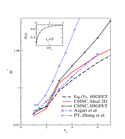
Figure 7: The effective mass $m^{*}_{H}$ in a HIGFET. The PT results of Zhang et al., and Asgari et al., for the HIGFET are close to the ideal-2D results from QMC. The “unperturbed-$g$” approach to the energy using CHNC-based PDFs gives a slight reduction from the ideal 2D. For the full CHNC calculation, see Fig. 8

In Fig. 7 we present a comparison of various theoretical calculations of the effective mass $m^{*}_{H}$ of the electrons in the HIGFET. The PT calculations of Zhang et al., and Asgari et al., show a strong decrease of $m^{*}$ from the PT values in the ideal 2DES. Our calculations, using the “unperturbed-$g$” approximation, Eq. 26, lead to a $m^{*}_{H}$ which is only slightly reduced by the thickness effect. This $m^{*}_{H}$ curve is in close to that of Asgari et al. This is clearly a numerical accident. According to Asgari et. al., the difference between the ideal $m^{*}$ and $m^{*}_{H}$ increase as $r_{s}$ increases. In our calculation using the “unperturbed-$g$” approximation, the difference, already quite small, seems to diminish as $r_{s}$ increases. In fact, as $r_{s}$ increases, the ratio $w/r_{s}$ of the HIGFET layer decreases and the thickness effect may be expected to decrease, unless the difference between $m^{*}$ and $m^{*}_{H}$ is driven by some other effect. This “other effect” is revealed by giving up the “unperturbed-$g$” approximation, and using the full thick-layer 2DES pair-distribution function at finite $T$, calculated using the CHNC, to evaluate the total free energy $F(r_{s},T)$ of the quasi-2D system, and hence the $m^{*}_{H}$. In Fig. 8 we display the PDF of the quasi-2DES of a HIGFET at $r_{s}=5$, and compare it with the PDF of the ideal 2DES. The difference between the ideal and quasi systems is embodied in the form factor $F(r)$. The reduced Coulomb repulsion at small-$r$ leads to a large pile-up of electrons around the electron at the origin. This means, the electron has to drag this charge pileup and this contributes an enhanced $m^{*}$ to the thermodynamic and transport properties of the quasi 2DES.

The experimental results of Tan et. al., for $m^{*}$ show an increase of $\sim$ 150% between $r_{s}$=3 and $r_{s}=6$. Our results from the full CHNC calculation, as well as the perturbation results of Asgari et al., are shown in the lower panel of Fig. 8. Given the failure of the PT calculations to reproduce the QMC-based $m^{*}$ for the ideal 2D, it is difficult to evaluate the reliability of the PT-based $m^{*}_{H}$. The PT-overestimate of $m^{*}$ of the ideal 2D is typical of the RPA-like character of these theories which are likely to predict spin transitions at relatively high densities. Also, we believe that if the same PT prescriptions were used to evaluate the one-top value $g(0)$ of the PDFS of the 2DES and the quasi-2DES, another measure of the short-comings of the PT methods would be revealed.

V.2 Enhanced spin susceptibility and the Lande-$g$ factor.

The product $m^{*}g^{*}$ is given by the ratio of the static spin susceptibility $\chi_{s}$ to the ideal (Pauli) spin susceptibility $\chi_{P}$. The long wavelength limit of the static response functions are connected with the compressibility or the spin-stiffness via the second derivative of the total energy with respect to the density or the spin polarization2valley . De Palo et al.morsen have calculated $m^{*}g^{*}$ from the QMC pair distribution functions and shown that they obtain quantitative agreement with the data for very narrow 2-D systemsvakili as well as for the thicker systems found in HIGFETSzhu . The CHNC PDFs are close approximations to QMC results, and when used in Eq. 26, yield correction energies which are in good agreement with the energies obtained by De Palo et aldepalo . In Ref. 2valley we showed that the rapid enhancement of $m^{*}g^{*}$ in Si/SiO₂ 2DES is a consequence of the increase in $m^{*}$ with $r_{s}$, and that the $g^{*}$ does n͡ot increase with $r_{s}$ because there is no spin-phase transition in the 2-valley case. In the HIGFET system there is a slightly delayed SPT, as seen in Fig. 5. Hence $m^{*}g^{*}$ increases with $r_{s}$, while $m^{*}$ also increases quite rapidly, due to the enhanced “on-top” correlations shown (Fig. 8) in the PDF of the quasi-2DES. The resulting $g^{*}$ of the HIGFET is shown in Fig. 9.

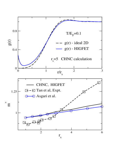
Figure 8: (a)The spin-averaged $g(r)$ at $r_{s}=5$ and $T/E_{F}$=0.1, for an ideal 2DES, and for a HIGFET calculated using CHNC. (b)The effective mass $m^{*}_{H}$ in a HIGFET from fully self-consistent CHNC calculations finite-$T$. The experimental data are from Tan et altan .

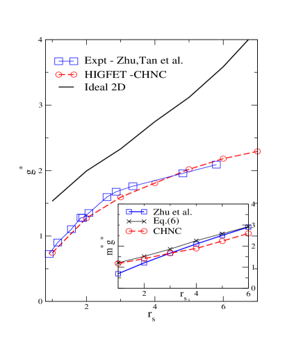
Figure 9: The ideal 2DES $g$-factor is obtained from the QMC $m^{*}g^{*}$ of ref. attac , divided by the CHNC ideal 2D $m^{*}$. The experimental HIGFET $g_{H}^{*}$ (boxes) is from the $m^{*}g^{*}$ of Zhu et al., divided by the $m^{*}$ of Tan et al. The inset shows the spin-susceptibility enhancement $m^{*}g^{*}$ from the $E_{xc}(r_{s},\zeta)$ calculated from Eq. 26, where the ideal 2D $g(r,w=0)$ is used, and from the full CHNC calculation using the $g(r,w)$ consistent with the quasi-2D potential.

VI Conclusion.

We have presented a detailed study of the effect of many-body interactions in quasi-2D electron layers using a single theoretical framework which involves the calculation of the pair-distribution functions of the system via a classical representation of the quantum fluid. A procedure for replacing the inhomogeneous transverse distributions via a constant-density model, i.e., an equivalent homogeneous distribution, has also been demonstrated. Easy to use parametrized fit formulae for the exchange energy at zero and finite-$T$ have been presented. A simple numerical scheme for calculating the correlation energy of a thick 2D layer,, via a 3-D slab model combined with a 1-D rod model, has also been demonstrated. We find that the thickness effect on the spin-phase transition etc., provides a clear picture of the changes in the spin-susceptibility enhancement leading to a strong increase in the $g$-factor, while $m^{*}$ is increased due to the enhancement of the “on-top” correlations arising from the reduction of the Coulomb potential in thick layers. However, unlike in the case of the effective mass data for Si/SiO₂ systemsshash ; eplmass , these results do not provide good quantitative agreement with the effective-mass data for HIGFETS recently reported by Tan et al. This may be due to our use of the ideal 2DES bridge function even for the HIGFETS.

References

- (1) S. V. Kravchenko and M. P. Sarachik, Rep. Prog.Phys. 67, 1 (2004)
- (2) T. Ando, B. Fowler, and F. Stern, Rev. Mod. Phys. 54, 437 (1982)
- (3) J. Zhu, H. L. Stormer, L. N. Pfeiffer, K. W. Baldwin, and K. W. West, Phys. Rev. Lett. 90, 56805 (2003)
- (4) P. J. Poole, J. McCaffrey, R.L. Williams, J. Lefebvre, J. Vac. Sci. & Tech. B 19, 1467 (2001)
- (5) Y-H Kim, I-H Lee, S. Nagaraja, J-P Leburton, R. Q. Hood, R. M. Martin, Phys. Rev. B 61, 5202 (2000)
- (6) F. Stern, Jpn. J. Appl. Phys. Suppl. 2, 323 (1974)
- (7) J. F. Dobson and J. Wang, Phys. Rev. B 69, 235104 (2004) J. P. Perdew and Y. Wang, Phys. Rev B 45, 13244 (1992)
- (8) A. H. MacDonald and G. C. Aers, Phys. Rev. B 29, 5976 (1984)
- (9) F. C. Zhang and S. Das Sarma, Phys. Rev. B 33, 2903 (1986)
- (10) E. Tutuc, S. Melinte, E. P. de Poortere, M. Sheyegan, and R. Winkler. cond-mat/0301027
- (11) Y.-W Tan, J. Zhu, H. L. Stormer, L. N. Pfeiffer, K. N. Baldwin, and K. W. West, cond-matt/0412260
- (12) S. De Palo, M. Botti, S. Moroni, and G. Senatore, cond-mat/0410145
- (13) R. Asgari, B. Davoudi, M. Polini, M. P. Tosi, G. F. Giuliani, and G. Vignale, Phys. Rev. B 71, 45323 (2005); cond-mat/0412665
- (14) Y. Zhang and S. Das Sarma, Phys. Rev. B 71,45322 (2005); cond-mat/0312565
- (15) M. W. C. Dharma-wardana, cond-mat/503246
- (16) D. J. W. Geldart and S. Vosko, Van. J. Phys.
- (17) Y. Kwon, D. M. Ceperley, and R. M. Martin, Phys. Rev. B 50, 1684 (1994)
- (18) K. S. Singwi, M. P. Tosi, R. H. Land, Pnd A. Sjolander, Phys. Rev B 176, 589 (1968)
- (19) S. Ichimaru, Rev. Mod. Phys. 54, 1017 (1982)
- (20) M. W. C. Dharma-wardana and F. Perrot, Phys. Rev. Lett. 84, 959 (2000)
- (21) François Perrot and M. W. C. Dharma-wardana, Phys. Rev. B, 62, 14766 (2000)
- (22) François Perrot and M. W. C. Dharma-wardana, Phys. Rev. Lett. 87, 206404 (2001)
- (23) M. W. C. Dharma-wardana and F. Perrot., Phys. Rev. Lett. 90, 136601 (2003)
- (24) M. W. C. Dharma-wardana and F. Perrot, Phys. Rev. B, 66, 14110 (2002)
- (25) M. W. C. Dharma-wardana and F. Perrot, Phys. Rev. B 70, 035308 (2004)
- (26) M. W. C. Dharma-wardana and F. Perrot, Europhys. Lett. 63, 660-666 (2003)
- (27) M. W. C. Dharma-wardana, Europhys. Lett. 67, 552 (2004)
- (28) F. Lado, J. Chem. Phys. 47, 5369 (1967)
- (29) Y. Rosenfeld, Phys.Rev. A bf42, 5978 (1990), M. Baus, J.-P Hansen J. Phys. C: Solid State Phys. 19, L463 (1986); our Fortran codes are available from the author.
- (30) C. Bulutay and B. Tanatar, Phys. Rev. B 65, 195116 (2002) N. Q. Khanh and H. Totsuji, Solid State Com., 129,37 (2004)
- (31) F. F. Fang and W. E. Howard, Phys. Rev. lett. 16, 797 (1966)
- (32) P. Gori-Giorgi and A. Savin, cond-mat/0411179 These authors have proposed the same inhomogeneoushomogeneous mapping and applied it to 2-electron atomic systems.
- (33) Daniel Jost and M. W. C. Dharma-wardana (unpublished)
- (34) F. Perrot and M. W. C. Dharma-wardana, Phys. Rev. A 30, 2619 (1984)
- (35) We thank Stephania de Palo and Gaetano Senatore for informative and helpful correspondence, and for providing us with their correction energy and the full diffusion-QMC correction at .
- (36) P. Gori-Giorgi, S. Moroni and G. B. Bachelet, Phys. Rev. B 70, 115102 (2004)
- (37) L. Samaj, cond-mat/0402027
- (38) D. M. Ceperley and B. J. Alder, Phsy. Rev. Lett. 45, 566 (1980)
- (39) P. Gori-Giorgi and J. P. Perdew, PRB 69, 041103 (2004)
- (40) A. A. Shashkin, M. Rashmi, S. Anissimova, and S. V. Kravchenko, V. T. Dolgopolov, T. M. Klapwijk, Phys. Rev. Lett. 91, 46403 (2003)
- (41) K. Vakili, Y. P. Shkolnikov, E. Tutuc, E. P. de Poortere, and M. Shayegan, Phys. Rev. Lett. 92,226401 (2004)
- (42) M. W. C. Dharma-wardana, Solid State Com. 127, 783-788 (2003)
- (43) C. Attaccalite et al., Phys. Rev. Lett. 88, 256601 (2002)