Condensation and vortex formation in Bose-gas upon cooling

Abstract

The mechanism for the transition of a Bose gas to the superfluid state via thermal fluctuations is considered. It is shown that in the process of external cooling some critical fluctuations (instantons) are formed above the critical temperature. The probability of the instanton formation is calculated in the three and two-dimensional cases. It is found that this probability increases as the system approaches the transition temperature. It is shown that the evolution of an individual instanton is impossible without the formation of vortices in its superfluid part.

I Introduction

The ideas of the kinetics of phase transitions have been thoroughly developed for first-order phase transitions and envisage the existence of the metastable phase itself and an equilibrium critical nucleus. The corresponding theory was worked out in Bec , Zel and described in detail in Lan . However, theoretical concepts concerning the kinetics of second-order phase transitions, where these two facts do not exist, have been developed insufficiently. In the Lif was proposed a certain special model for the formation of an ordered phase after the fast phase-transition stage in the ”short-range” order in the presence of only two types of ordering.

The interest in the problem of a phase transition upon a fast change in external parameters (e.g., temperature) has been aroused in connection with the cosmological ideas of the Big Bang, where the rapidly expanding Universe must be cooled and pass through a series of phase transformations accompanied by a change in the symmetry of physical fields Zell . It was proposed that the kinetics of these transformations can be modeled in condensed matter Kib .

In the Zur was proposed a theory of the second-order phase transition upon a rapid change in temperature in liquid ${}^{4}\rm{He}$. The main assumption in the proposed mechanism is about the ”critical retardation” of all processes in the vicinity of the transition temperature and ”fast” formation of the nuclei of a new phase upon the subsequent cooling. This gives rise to a large number of defects on the order of the number of fluctuations far above the transition point.

However, no retardation in the formation of a new phase has been detected experimentally; the critical retardation is associated with the duration of the equilibration process at macroscopic distances, which is insignificant for the nonuniform process of formation of a new phase.

In this work, we consider the transition to a new phase via the evolution of fluctuations on scales much smaller than the correlation length, which can occur quite rapidly even in the vicinity of the critical temperature. The transition kinetics in this case is found to be directly related to the cooling process itself. In our preliminary paper BIS this approach was proposed for the specific problem of Bose condensation of a weakly interacting Bose gas. The appropriate set of equations governing critical fluctuations was derived. In the present work a detailed analysis of the main equations is performed including numerical calculations and a generalization to the case of the two-dimensional exciton gas. We will consider the formation of a condensate in the model of a weakly nonideal Bose gas with external cooling and demonstrate an analogy with first-order phase transitions.

A similar approach to the problem of the wave nucleation rate due to thermal noise was considered in Henry . But the problem of the present work requires the noise to be connected to the random thermal fluxes. In this case it is appropriate to use a more general approach for the instanton formation namely local Hamilton equations rather than the Lagrangian equations used in Henry (see also Marder ). In Cher the problem of large negative gradients in Burgers turbulence was considered, which has some resemblance to the differential equations discussed in our work, but the boundary problem is quite different.

II Dilute Bose-gas upon cooling

The standard theory of a weakly nonideal Bose gas involves a Hamiltonian of the form :

$$\hat{H}=\sum\limits_{p}\frac{\hat{p}^{2}}{2m}\hat{a_{p}}^{+}\hat{{a}_{p}}+\frac{2\pi\hbar^{2}a_{0}}{m}\sum\limits_{p}\hat{{a}_{p_{4}}}^{+}\hat{{a}_{p_{3}}}^{+}\hat{{a}_{p_{2}}}\hat{{a}_{p_{1}}},$$ (1)

where $a_{0}$ – is the scattering amplitude having the atomic scale and $m$ – is the atomic mass. The properties of such gas for a small density $n$ (determined by the gas parameter $\eta=n{a_{0}}^{3}\ll 1$ ) are close to the properties of an ideal Bose gas with the transition temperature Ld :

$$T_{c}=\frac{3.31}{\sqrt{2}}\frac{\hbar^{2}n^{2/3}}{m}.$$ (2)

At temperatures below the transition point, the ideal Bose gas has a pressure depending only on the temperature:

$$P_{id}=0.0851\frac{m^{3/2}T^{5/2}}{\hbar^{3}},$$ (3)

which corresponds to zero isothermal sound velocity.

Considering the finite scattering amplitude we can write the qualitative equation of state below the transition point as

$$P=P_{id}(T)+\frac{\hbar^{2}a_{0}n^{2}}{m}.$$ (4)

We omitted the insignificant constant factor in the second term.

The entire kinetics is essentially determined by the Bose-gas cooling mechanism. We will consider a simple model where the Bose gas is in a certain solid matrix with which it only slightly interacts. Such a situation may take place, for example, for the exciton gas in a crystal. The crystal can be rapidly cooled to a low temperature; in this case, the Bose-gas cooling proceeds via phonon emission. Assuming that the heat capacity of the crystal is large compared to the Bose gas, we can disregard the presence of thermal phonons in the crystal and their effect on the Bose gas. As a result, we obtain a uniform energy-loss mechanism, which is described by a phenomenological quantity $T/\tau_{ph}$. The other models of cooling necessitate the analysis of heat transfer at the sample boundaries, which is a much more complicated problem. The loss rate $1/{\tau_{ph}}$ is determined by the collisions of particles with each other and by the interaction with phonons, which will be regarded as weak:

$$1/\tau_{ph}\ll 1/\tau_{tr}.$$

Since $1/\tau_{ph}\sim nv_{T}\sigma_{ph}$ , $1/\tau_{tr}\sim nv_{T}{a_{0}}^{2}$ ($v_{T}$ s the thermal velocity), this means that

$$\sigma_{ph}\ll{a_{0}}^{2},$$

where $\sigma_{ph}$ is the cross section for scattering with phonon emission, which corresponds to the weak interaction of Bose gas with the crystal.

In view of the smallness of quantity $1/{\tau_{ph}}$ the evolution of the Bose system is slow; in particular, we assume that the acoustic wavelength $c\tau_{ph}\sim v_{T}\tau_{ph}$ is large compared to the characteristic length $\sim\sqrt{\chi\tau_{ph}}$ , where $\chi$ - is the thermal diffusivity:

$$\frac{\sqrt{\chi\tau_{ph}}}{v_{T}\tau_{ph}}\sim\sqrt{\frac{l^{2}}{{v_{T}}^{2}\tau_{tr}\tau_{ph}}}\sim\sqrt{\frac{\tau_{tr}}{\tau_{ph}}}\ll 1$$ (5)

($l$ stands for the mean free path). This makes it possible to assume that the fluctuation evolution occurs at a constant pressure that coincides with the thermodynamically equilibrium pressure.

It follows from Eq.(4) that the density variation $\delta n$ in the fluctuation region is related to a change in temperature by

$$\frac{\delta n}{n}=-\frac{\delta T}{T}\frac{1}{\eta^{\frac{1}{3}}}.$$ (6)

The relative density fluctuation is large compared to the relative temperature fluctuation in the temperature range $T<T_{c}$. This leads to a rapid increase in the reciprocal phonon time

$$\delta\frac{1}{\tau_{ph}}\sim-\frac{\delta T}{T}\frac{1}{\eta^{\frac{1}{3}}}\frac{1}{{\tau_{ph}}^{0}}$$ (7)

(where $1/{{\tau_{ph}}^{0}}=nv_{T}\sigma_{ph}$) with decreasing temperature and enhancement of cooling in the fluctuation region. For this reason, we will disregard the phonon emission in the region far from the developed fluctuations, assuming that

$$\frac{1}{\tau_{ph}}\sim-\frac{\delta T}{T_{c}}\frac{1}{\eta^{\frac{1}{3}}}\frac{1}{{\tau_{ph}}^{0}}U(T_{c}-T),$$ (8)

where $U(T_{c}-T)=1$ for $\delta T=T-T_{c}<0$ and $U(T_{c}-T)=0$ for $T-T_{c}>0$.

This allows us to consider the problem of fluctuation kinetics within the framework of the theory of hydrodynamic fluctuations by supplementing the hydrodynamic equations with the energy flux carried away as a result of phonon emission:

$$\frac{T}{{\tau_{ph}}^{0}}\frac{\delta n}{n}=-\frac{T_{c}-T}{{\tau_{ph}}}U(T_{c}-T),$$ (9)

where $1/{\tau_{ph}}=(1/{\tau_{ph}}^{0})(1/\eta^{1/3})$. In view of the constancy of pressure, we can describe the evolution of temperature fluctuations by the heat conduction equation

$$nc_{p}\left(\frac{\partial T}{\partial t}\!+\!\vec{v}\frac{\partial T}{\partial\vec{r}}\right)\!=\!\nabla(\varkappa\nabla T)\!+\!\frac{T-T_{c}}{{\tau_{ph}}}nc_{p}U(T_{c}\!-\!T),$$ (10)

where the energy flux carried away by phonons is added, $\varkappa$ – is the heat conductivity, $c_{p}$ – is the specific heat per particle under a constant pressure. This equation contains the drift term with mass velocity $v({\bf r})$, which appears due to the high density in the fluctuation core. In the following analysis, this term will be omitted as a higher-order term in fluctuation. We are interested in the temperature-field fluctuations and their time evolution. To analyze these fluctuations, we must introduce random heat fluxes $\bf q$ Lan , Liff , i.e., the Langevin term ${\bf\nabla q}$. These fluxes are delta-correlated (i.e., correlated at distances and time intervals smaller than the hydrodynamic scales). In the case considered, this is ensured by the fact that the time $\tau_{ph}$ and distance $\sqrt{\chi{\tau_{ph}}}$ ($\chi$ – is thermal diffusivity) are larger than the microscopic characteristics.

The probability $W_{t}(T(r))$ of realizing the given configuration $T(r)$ fluctuation field at time $t$ obeys the Fokker-Planck equation in variational derivatives Kl

$$\frac{\partial}{\partial t}W=-\int\frac{\delta}{\delta T(r)}\Big{[}\frac{\chi{T_{\infty}}^{2}}{nc_{p}}{\bf\nabla}^{2}\frac{\delta}{\delta T(r)}W$$

$$\qquad+\left[\chi{\nabla}^{2}T+U(T_{c}-T)\frac{T-T_{c}}{\tau_{ph}}\right]W\Big{]}d^{3}r.$$ (11)

In the absence of the interaction with phonons, the stationary solution to this equation coincides with the result obtained in the thermodynamic theory of fluctuations. The quantity

$$\chi{\bf\nabla}^{2}T+U(T_{c}-T)\frac{T-T_{c}}{{\tau_{ph}}}=\frac{\partial T}{\partial t}$$ (12)

is the temperature-variation rate upon the deviation from the mean value $T=T_{\infty}$.

We assume that fluctuations occur at a fixed temperature $T_{\infty}>T_{c}$. Fluctuations with $\triangle T=T-T_{\infty}\ll T_{\infty}$ occur quite frequently and are characterized by a certain (in fact, stationary) spatial distribution that determines the value of $W_{t}(T)$. In view of the normalization, the latter quantity gives the number of small fluctuations in a unit volume. However, rare large-amplitude fluctuations with $T{\sim}T_{c}-T_{\infty}$, $T<T_{c}$, also sometimes occur, initiating the effective cooling by phonons, so that the fluctuation becomes irreversible and the nucleus of a new phase appears. Our goal is to calculate the probability of such fluctuations in a unit volume per unit time. Since they are infrequent and the distribution at small $T_{\infty}-T$ is stationary, one can use the method of characteristics to determine the exponentially low probability of formation of such a nucleus (instanton for the Fokker-Planck equation). An important difference from the theory of nucleation in the first-order phase transition is that the probability of instanton formation in this case is determined by the cooling process.

III A toy model

To clarify the situation, let us consider the instanton solution in the case of one degree of freedom, for which the Fokker-Planck equation has the form

$$\frac{\partial W}{\partial t}=\frac{\partial}{\partial x}\left(D\frac{\partial W}{\partial x}-vW\right),$$ (13)

where $D$ is the constant diffusion coefficient and $v(x)$ is the macroscopic variation rate of the quantity $x$ with allowance for its relaxation upon the deviation from equilibrium and for an external effect (analogue of phonon emission). Setting $W=e^{S}$, and assuming that the moduli of S and its first derivative are large, we obtain, to leading terms, the equation

$$\frac{\partial S}{\partial t}=D{\left({\frac{\partial S}{\partial x}}\right)}^{2}-v\frac{\partial S}{\partial x}-\frac{\partial v}{\partial x}.$$ (14)

This is the Hamilton-Jacobi equation with the Hamiltonian (${\partial S}/{\partial x}=p$)

$$H({\frac{\partial S}{\partial x}},x)=-Dp^{2}+pv+\frac{\partial v}{\partial x}.$$ (15)

The Hamilton equations are the characteristics of this equation in partial derivatives,

$$\frac{dx}{dt}=-2Dp+v,$$ (16)

$$\frac{dp}{dt}=-{\frac{dv}{dx}}p-\frac{d^{2}v}{d^{2}x}.$$ (17)

The contribution of the velocity divergence to the Hamiltonian is significant only in the vicinity of the point $v=0$. We are interested in the special solution that passes through the equilibrium point $p=0$, $v=0$. In the 1D Fokker-Planck equation, one can eliminate the term with a first derivative by substitution; in this case, we have an analogy with quantum mechanics and can use the well-known results. Nevertheless, we will use direct estimates in the vicinity of $v=0$.

In the Hamilton equation, the energy is conserved. In view of the smallness of the divergence term, this gives $H=-Dp^{2}+pv=0$, whence $p=v/D$ and

$$S=-\int\frac{v^{2}}{D}dt=\int\limits_{0}\limits^{x^{*}}\frac{v}{D}dx.$$ (18)

We assume that the velocity $v(x)$ is a convex-down function with two zeros (stable at zero and unstable at $x^{*}$ ($x^{*}>0$). Such a shape of the function $v(x)$ is ensured by the entire cooling process, including phonon emission. For $x>x^{*}$, the solution tends to larger values of x, while the action is gathered from zero to $x^{*}$, where $v<0$. In the vicinity of $x^{*}$, we must take into account the quantity ${dv}/{dx}$ . For large values of $x$, $p^{2}$ can be ignored, yielding $p\approx-{({dv}/{dx})}/v$,

$$S\sim S_{0}-\ln(v/v_{0}),$$ (19)

where $v_{0}$ is the effective velocity in the region where the solutions for $x<x^{*}$ and $x>x^{*}$ match. The solution $S_{0}$ itself has the form $e^{S}\approx{v_{0}}e^{S_{0}}/v$, and current $j\approx v_{0}e^{S_{0}}$. One can estimate the value of $v_{0}$, assuming that all terms in the Hamiltonian $H$ are of the same order of magnitude:

$$Dp^{2}\sim vp\sim\frac{dv}{dx}\sim\frac{v_{max}}{x^{*}}$$ (20)

which gives

$$v_{0}\sim\sqrt{\frac{D|v_{max}|}{x^{*}}}\sim\frac{|v_{max}|}{\sqrt{|S_{0}|}}.$$ (21)

In the many-dimensional case, the situation is the same,

$$\frac{dx^{i}}{dt}=-2D^{ij}p_{j}+v^{i},$$ (22)

$$\frac{dp_{i}}{dt}=-{\frac{\partial v^{k}}{\partial x^{i}}}p_{k}-\frac{\partial({\rm{div}}\vec{v})}{\partial x^{i}},$$ (23)

where $p=0$ at the beginning and $p\rightarrow 0$ at the end of the trajectory. Consequently, $|p|$ reaches its maximal value somewhere on the trajectory. At this point, the matrix ${\partial v_{i}}/{\partial x_{k}}$ has one zero eigenvalue and ${\bf p}$ is tangent to the corresponding eigenvector; subsequently, the trajectory passes to the neighborhood of the point corresponding to zero velocity $v$. This leads to the definition of the critical fluctuation (instanton) as a solution passing through the point ${\bf x}={\bf p}=0$, whereupon ${\bf p}\rightarrow 0$ for $|x|\rightarrow\infty$ as $1/v$, retaining the probability flux at a constant level.

IV Optimal fluctuation

An analogous procedure can be carried out for the field as well. In this case, the Hamiltonian has the form, in accordance with Eq.(II),

$$H\!=\!\int p({\bf r})\left[\frac{\chi{T_{\infty}}^{2}}{nc_{p}}{\bf\nabla}^{2}p({\bf r})\!+\!\chi{\bf\nabla}^{2}T\!+\!U(T_{c}-T)\frac{T-T_{c}}{{\tau_{ph}}}\right]d^{3}r$$ (24)

with the Hamilton equations

$$\frac{\partial T}{\partial t}=\frac{2\chi{T_{\infty}}^{2}}{nc_{p}}{\bf\nabla}^{2}p({\bf r})+\chi{\bf\nabla}^{2}T+U(T_{c}-T)\frac{T-T_{c}}{\tau_{ph}},$$ (25)

$$\frac{\partial p}{\partial t}=-\chi{\bf\nabla}^{2}p-\frac{p}{\tau_{ph}}U(T_{c}-T).$$ (26)

Here, $p={\delta S}/{\delta T({\bf r})}$. Eqs. (25), (26) define the critical fluctuation and can be reduced to dimensionless variables by the substitutions $\xi=r/\sqrt{\chi\tau_{ph}}$, $\tau=t/\tau_{ph}$,

$$\Theta=\frac{T-T_{c}}{T_{\infty}-T_{c}},~{}~{}p=\frac{nc_{p}(T_{\infty}-T_{c})\Pi}{{{T}^{2}}_{\infty}},$$

where $\Theta$ and $\Pi$ are the new dimensionless fields. In this case, the dimensionless equations have the form

$$\frac{\partial\Theta}{\partial\tau}={\bf\nabla}^{2}\Theta+\Theta U(-\Theta)+2{\bf\nabla}^{2}\Pi,$$ (27)

$$\frac{\partial\Pi}{\partial\tau}=-{\bf\nabla}^{2}\Pi-\Pi U(-\Theta).$$ (28)

The solution should fulfill the conditions $\Pi_{\xi\rightarrow\infty}\rightarrow 0$, $\Pi_{\tau\rightarrow-\infty}\rightarrow 0$, $\Theta_{\tau\rightarrow-\infty}\rightarrow 1$, $\Theta_{\xi\rightarrow\infty}\rightarrow 1$ and pass through the neighborhood of ${\partial\Theta}/{\partial\tau}\approx 0$, $\Pi\approx 0$ at $\tau\rightarrow\tau^{*}$. Later the fluctuation is developed by cooling, while the random fluxes can be neglected and ${\partial\Theta}/{\partial\tau}\approx{\bf\nabla}^{2}\Theta+\Theta U(-\Theta)$. With exponential precision we can assume that ${\partial\Theta}/{\partial\tau}\rightarrow 0$ at $\tau\rightarrow+\infty$, and $\Theta$ tends to the stationary solution $\Theta_{st}$ of the thermal diffusion equation, Eq.(27):

$$\Theta_{st}=\sin(\xi)/\xi,~{}\xi<\pi~{},$$

$$\Theta_{st}=1-\pi/\xi,~{}\xi>\pi~{}.$$ (29)

The difficulties with the numerical solution of this boundary value problem are due to the instability of Eq.(28) for ascending time whereas Eq.(27) is unstable for descending time. Therefore, it is impossible to find numerically the solution of the Cauchy problem in either direction of time. We briefly describe our adopted procedure. At early stages of the evolution, when $\Theta>0$ everywhere in space, it is easy to check the validity of the relation

$$\Theta=1-\Pi,$$ (30)

which coincides with the thermodynamical theory of temperature fluctuations. The function $\Pi$ grows with time according to Eq. (28) (thermal diffusion equation with negative time derivative). We can assume that at $\tau=0$ the maximum of $\Pi$ will reach 1. After this Eq. (30) is no longer valid. We can consider Eq. (28) as a Schroedinger equation with imaginary time and $\Pi\rightarrow 0$ at infinite time. At large $\tau$, the function $\Theta$ will be close to the stationary solution, Eq.(IV), which becomes zero at $\xi=\pi$. This means that $\Pi$, at large $\tau$, has an asymptotic proportional to

$$\Pi_{inf}=\exp{(-|\lambda|\tau)\Psi_{\lambda}},$$ (31)

where $\Psi_{\lambda}$ corresponds to the eigenfunction with the negative eigenvalue, $\lambda=-0.4576$, according to the Schroedinger equation with the potential $-U(\pi-\xi)$ (all other states will grow with $\tau$).

Let us denote by $r^{*}(\tau)$ the space-point for which $\Theta=0$ at time $\tau$. The curve $r^{*}(\tau)$ is a function of $\tau$ starting at small $\tau$ as square root of $\tau$ (because $\Theta$ has a minimum at $\xi=0$) and tending exponentially to $\pi$ at large $\tau$ (according to the Schroedinger-equation analogy, Eq.(31)). We don’t know the exact form of $r^{*}(\tau)$ but we can choose some probe function with the same asymptotic behavior. Having such a probe function, we can numerically solve Eq.(28) integrating it backward in time (it is unstable while integrating it forward in time) with the condition $\Pi_{inf}=\alpha\Psi_{\lambda}$ (of form Eq. (31)) (the prefactor $\alpha$ should be chosen to satisfy Eq. (30) at $\tau=0$).

Using this function $\Pi$, we can numerically solve Eq. (27) in two space-time regions independently. The first one is the internal region $\xi<r^{*}(\tau)$ the other one is $\xi>r^{*}(\tau)$ (the external region). $\Theta\rightarrow 1$ for $\xi\rightarrow\infty$ (for the external region) and $\Theta(r^{*})=0$ (for the both regions). For the exact function $r^{*}$ the space derivative $\Theta^{{}^{\prime}}={\partial\Theta}/{\partial\xi}$ will be continuous. For our probe function $r^{*}$ there will be some jump of the space derivative $\Theta^{{}^{\prime}}$ at $r^{*}(\tau)$. Thus, after performing the calculations, we will have in general a nonzero jump-function

$$\Delta\Theta^{{}^{\prime}}=\Theta^{{}^{\prime}}(r^{*}-0)-\Theta^{{}^{\prime}}(r^{*}+0)$$

depending on the choice of the curve $r^{*}$. Afterwords we should search for a more exact $r^{*}$ in order to minimize $max|\Delta\Theta^{{}^{\prime}}|$. Some steps within the framework of this procedure have been performed.

We use a space-time grid 2000x2000. The grid spacing was taken as $\delta\xi=0.015$ for the space coordinate and $\delta\tau=0.01$ for the time coordinate. First, we perform calculations backward in time for $\Pi$ using a standard implicit numerical scheme where the space derivatives are calculated for the final time of each time step. There are some modifications of the space grid in the vicinity of $r=r^{*}(t)$, for a better finite difference representation of the Laplacian. Then we use the analogous scheme for Eq.(27) and find $\Theta$ in the internal and external regions integrating forward in time and obtain $\Delta\Theta^{{}^{\prime}}$. We have defined our probe function $r^{*}(t)$ by a number of parameters. To obtain an exact solution we need, of course, an infinite number of parameters. In practice, for a reasonable precision we only need a few. The simplest form which obeys the asymptotic behavior is

$$r^{*}=\alpha\sqrt{\tau}+\beta\tau,~{}\tau<\tau_{0},$$

$$r^{*}=\pi-\delta\exp{(-|\lambda|\tau)},~{}\tau>\tau_{0}.$$

The parameters should be chosen such that $r^{*}$ is continuous and smooth at $\tau=\tau_{0}$. This means that we have two free parameters in this case (e.g. $\alpha$ and $\tau_{0}$). After minimization of $max|\Delta\Theta^{{}^{\prime}}|$ with respect to these two parameters we find right and left derivatives $\Theta^{{}^{\prime}}(r^{*}\pm 0)$ (see Fiq.1).

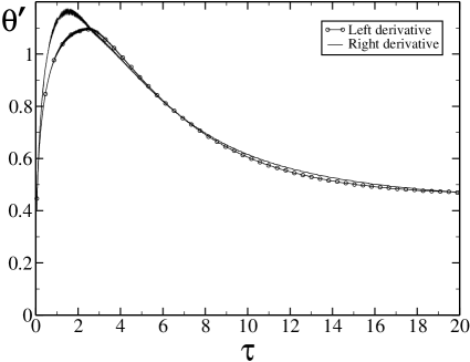
Figure 1: Left and right derivatives at $r^{*}$ for two free parameters

We can improve our results adding a new term $\gamma\tau^{2}$:

$$r^{*}=\alpha\sqrt{\tau}+\beta\tau+\gamma\tau^{2},~{}\tau<\tau_{0},$$

$$r^{*}=\pi-\delta\exp{(-|\lambda|\tau)},~{}\tau>\tau_{0}.$$ (32)

We have found that for $\alpha=2.28$, $\gamma=0.016$, $\tau_{0}=2.55$ there is an acceptable minimum of $|\Delta\Theta^{{}^{\prime}}|$ (see Fig.2). The corresponding jump-functions $\Delta\Theta^{{}^{\prime}}$ for the two and three parameter cases (for comparison) are plotted in Fig.3. One can see that the inclusion of this additional term decreases the maximum deviation, $max[|\Delta\Theta^{{}^{\prime}}|]$, by a factor of 3.

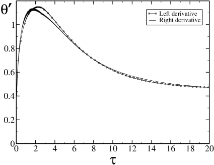
Figure 2: Left and right derivatives at $r^{*}$ for three free parameters

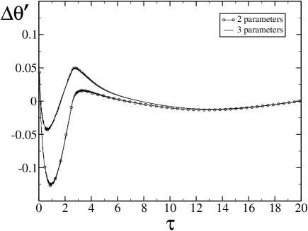
Figure 3: Jump-function $\Delta\Theta^{{}^{\prime}}(r^{*})$ for two and three free parameters

V The optimal fluctuation probability

The solution of Eqs. (27),(28) allows us to calculate the action

$$S = \int p\frac{\partial T}{\partial t}d^{3}rdt-\int Hdt$$

$$= s_{0}\frac{nc_{p}{(T_{\infty}-T_{c})}^{2}}{2{{T}^{2}}_{\infty}}{(\sqrt{\chi\tau_{ph}})}^{3}.$$ (33)

The negative constant $s_{0}$ is the dimensionless action

$$s_{0}=\int\limits_{-\infty}\limits^{\infty}d\tau\int\partial_{\tau}\Theta\Pi d^{3}\xi-\int\limits_{-\infty}\limits^{\infty}H_{1}d\tau,$$ (34)

where the space integral is taken over the whole space. Here

$$H_{1}\!=\!\int\Pi({\bf r})\left[{\bf\nabla}^{2}\Pi({\bf r})\!+\!{\bf\nabla}^{2}\Theta\!+\!U(-\Theta)\Theta\right]d^{3}\xi$$ (35)

is the dimensionless Hamiltonian, Eq.(24). The negative constant $s_{0}$ is a universal number corresponding to the largest action $S_{0}$ and is independent of the values of physical constants and the difference $T_{\infty}-T_{c}$.

From Eq.(27) and from the expression for the Hamiltonian, Eq. (35), it is easy to see that

$$s_{0}=\int\limits_{-\infty}\limits^{\infty}d\tau\int\Pi\nabla^{2}\Pi d^{3}r$$

for a smooth solution of Eqs.(27), (28). In our case, the jump of $\Theta$ derivatives should be taken into account which modifies the action :

$$s_{0}=\int\limits_{-\infty}\limits^{\infty}d\tau\int\Pi\nabla^{2}\Pi d^{3}\xi-\int\limits_{-\infty}\limits^{\infty}d\tau\int\int\Delta\Theta^{{}^{\prime}}\Pi dS_{r^{*}}.$$

The surface integral should be taken over a sphere of radius $r^{*}$. Using Eq. (28),

$$\nabla^{2}\Pi=-\partial_{\tau}\Pi-U(r^{*}-\xi)\Pi,$$

we finally find for the action

$$s_{0}=-\int\limits_{-\infty}\limits^{\infty}d\tau\int\limits_{\xi<r^{*}}\Pi^{2}d^{3}\xi-\int\limits_{-\infty}\limits^{\infty}dt\int\int\Delta\Theta^{{}^{\prime}}\Pi dS_{r^{*}}$$ (36)

Substituting the results of the numerical calculations we get

$$s_{0}=-100.73.$$

Test results for a smaller grid spacing, $\delta\xi=0.003$, give

$$s_{0}=-100.23$$

with a negligible jump-function, $\Delta\Theta^{{}^{\prime}}$. These results are in agreement with the naive estimate from Eq.(36): The characteristic scale of $\Pi^{2}$ is 1 and the action is proportional to the volume of a sphere of radius $\pi$, which is about 100.

To estimate the temperature-variation rate, one can take

$$|v_{max}|=\frac{T_{\infty}-T_{c}}{\tau_{ph}}{(\sqrt{\chi\tau_{ph}})}^{3}n.$$ (37)

In this case, in accordance with Eq. (21), one can write for the probability flux in the transition region

$$j\sim\frac{T_{\infty}{(n{\left(\sqrt{\chi\tau_{ph}}\right)}^{3})}^{\frac{1}{2}}}{\tau_{ph}c_{p}}e^{S}\nu.$$ (38)

The constant $\nu$ cannot be estimated from the theory of hydrodynamic fluctuations PiT . This quantity gives the number of small equilibrium fluctuations with $\delta T\ll T$ in a unit volume on the atomic scale. As an estimate, we can use the relation $\nu={n}/T_{\infty}$ . Thus, the number of critical fluctuations per unit time in a unit volume is

$$\frac{dN}{dt}\sim\frac{n{(n{{\left(\sqrt{\chi\tau_{ph}}\right)}^{3})}^{1/2}}}{\tau_{ph}c_{p}}\exp\left[s_{0}\frac{nc_{p}{(T_{\infty}-T_{c})}^{2}}{2{{T}^{2}}_{\infty}}{(\sqrt{\chi\tau_{ph}})}^{3}\right].$$ (39)

The nuclei of a new phase are intensively formed as $T_{\infty}$ approaches $T_{c}$ and then grow rapidly. We have considered the initial phase of critical-fluctuation growth and restricted our analysis to the heat transfer via heat conduction, disregarding superfluidity effects at this stage. This approximation can be justified by the fact that the largest contribution to the action comes from the region lying far from the region of low velocities $v$, where $p({\bf r})={\delta S}/{\delta T({\bf r})}$ becomes small and the fluctuation contribution can be neglected because $W\sim v^{-1}e^{S_{0}}$.

VI Bose condensation in the two-dimensional case

Most experiments on Bose-condensation in exciton systems were done in the two-dimensional (2D) case because these excitons are more stable But ; Tim . Condensation into the superfluid state of interwell exctions in AlAs/GaAs structures was supposedly observed in But . In these experiments excitons were obtained in a 2D quantum well and were cooled by phonon emission into the 3D volume of the surrounding semiconductor SVI . We can expect our theory to be suitable to explain the formation of a condensate in this case. In such systems the Bose-gas of excitons is dilute ($n{a_{0}}^{2}\ll 1$) and has a long lifetime. There is no a true condensate at any nonzero temperature but it was shown in Pop that there is a superfluid transition at

$$T_{c}=\frac{2\pi n\hbar^{2}}{m\ln\ln(1/{n{a_{0}}^{2}})}.$$ (40)

According to Pop the pressure has the form:

$$P=\frac{2\pi n^{2}}{m\ln(1/{n{a_{0}}^{2}})}+\frac{mT^{2}\zeta(2)}{2\pi\hbar^{2}}.$$ (41)

As it was pointed out in fish these results hold only under the condition,

$$\ln\ln(1/{n{a_{0}}^{2}})\gg 1.$$ (42)

Using the analogy to the 3D case, we consider temperature fluctuations at constant pressure and generalize the results of previous sections to the 2D case. In these fluctuations below $T_{c}$ there is also an increase of the reciprocal phonon time, and in the 2D case Eq.(6) should be replaced by

$$\frac{\delta n}{n}=-\frac{\delta T}{T}\frac{\ln(1/(n{a_{0}}^{2}))}{{(\ln\ln(1/(n{a_{0}}^{2})))}^{2}}.$$ (43)

The large parameter ${(\ln(1/(n{a_{0}}^{2}))}/{{(\ln\ln(1/(n{a_{0}}^{2})))}^{2}}$ plays the role of $1/{{\eta}^{\frac{1}{3}}}$ in Eq. (6). Eventually, we arrive to the same set of equations, Eqs. (27-28), as in the 3D case. Thus, the number of critical fluctuations per unit time in a unit volume in the 2D case is

$$\frac{dN}{dt}\sim\frac{n{(n{{\chi\tau_{ph}})}^{1/2}}}{\tau_{ph}c_{p}}\exp\left[s_{0}\frac{nc_{p}{(T_{\infty}-T_{c})}^{2}}{2{{T}^{2}}_{\infty}}{(\chi\tau_{ph})}\right].$$ (44)

Numerical calculations in the 2D case are somewhat more complicated in comparison to the 3D case. There is no a stationary solution like Eq.(IV). However, if we consider the system of a finite size $R$, there will be an analog to Eq.(IV):

$$\Theta_{stat}=-\frac{J_{0}(\xi)}{{\lambda^{1}}_{0}J_{1}({\lambda^{1}}_{0})\ln(\frac{R}{{\lambda^{1}}_{0}})},~{}\xi<{\lambda^{1}}_{0},$$

$$\Theta_{stat}=\frac{\ln(\frac{\xi}{\lambda^{1}}_{0})}{\ln(\frac{R}{\lambda^{1}}_{0})},~{}\xi>{\lambda^{1}}_{0}.$$ (45)

Here $J_{n}$ is a Bessel function and ${\lambda^{1}}_{0}$ is the first zero of $J_{0}(x)$. We see that the negative values of $\Theta$ are logarithmically suppressed. This is not very important because the system after passing in the vicinity of the stationary point evolves further due to the divergence term (which was neglected in Eq.(24) and Eqs.(27),(28)). This term in Eq. (24) has the form

$$\Delta H=\int\frac{U(T_{c}-T)}{\tau_{ph}}d^{2}r.$$

The Hamilton equations, Eqs.(27),(28), should also be modified:

$$\frac{\partial\Theta}{\partial\tau}={\bf\nabla}^{2}\Theta+\Theta U(-\Theta)+2{\bf\nabla}^{2}\Pi,$$ (46)

$$\frac{\partial\Pi}{\partial\tau}= - {\bf\nabla}^{2}\Pi-\Pi U(-\Theta)+$$ (47)

$$\delta(-\Theta)\frac{{T_{\infty}}^{2}}{{(T_{\infty}-T_{c})}^{2}nc_{p}\chi\tau_{ph}}.$$

Here $\delta(-\Theta)$ is a delta-function. As in the toy-model, this term starts to play an important role at large $\tau$ while at small and intermediate $\tau$ it is unimportant. There is no need to take this term into account in our calculations of the action in the 3D case because it is a higher-order quasiclassical correction for the 3D instanton. But in the 2D case, we can consider the finite-time evolution due to this term. The large-time cutoff can be estimated by assuming that at this moment the divergence term becomes of the same order of magnitude as the main terms in Eq.(47). We know the large-time asymptotics of $\Pi$ in a finite-size system of radius $R$,

$$\Pi\rightarrow\alpha\Psi_{\lambda}(r)\exp(-|\lambda|\tau),$$

where $\Psi_{\lambda}(r)$ is the eigenfunction with the negative eigenvalue $\lambda$ of the 2D Schroedinger equation with the potential $-U({\lambda^{1}}_{0}-\xi)$. Using this asym

ptotics and comparing terms in the equation for the norm, $||\Pi||=\int\Pi^{2}d^{2}r$,

$$\partial_{\tau}\frac{||\Pi||}{2}=-|\lambda|*||\Pi||+\Pi({\lambda^{1}}_{0})\frac{{T_{\infty}}^{2}}{{(T_{\infty}-T_{c})}^{2}nc_{p}\chi\tau_{ph}},$$

we can estimate the large-time cutoff as:

$$\Delta\tau\sim\frac{1}{|\lambda|}\ln\left(\alpha|\lambda|\frac{{(T_{\infty}-T_{c})}^{2}nc_{p}\chi\tau_{ph}}{{T_{\infty}}^{2}}\right).$$

The space position of the thermal front, that corresponds to this time, is

$$\Delta r=\sqrt{\Delta\tau}.$$

If we choose the point $R$, where $\Theta(R)=1$, at the distance $\Delta r$ from the point $r^{*}$ (where $\Theta(r^{*})=0$ at the largest time), we can assume that the value of the total action will be almost independent of the exact position of $R$. We have performed a number of runs with different values of $R$ and have found no essential difference in the action. The resulting constant is

$$s_{0}=-13.6$$

The same naive estimate as in 3d can be performed. The action now is proportional $\pi{\left({{\lambda^{1}}_{0}}\right)}^{2}$ which is about 13.

VII The later stage of instanton growth

Analysis of the subsequent growth of the instanton requires the solution of hydrodynamic equations for a superfluid liquid, because a superfluid core appears in the developing fluctuation. We will qualitatively consider the phenomena that arise in this case. Proceeding from the assumption that the value of $\tau_{ph}$ is high, we assume that the motion in this region is quasi-stationary and tuned due to the slow cooling by phonons. We will use the hydrodynamic equations for a superfluid liquid in the vicinity of the transition point in the form proposed by Khalatnikov Hal :

$$\frac{\partial{\bf v}_{s}}{\partial t}=-\nabla\left(\frac{v_{s}^{2}}{2}+\mu+\mu_{s}\right),$$

$$\frac{\partial\rho}{\partial t}+{\rm{div}}(\rho_{s}{\bf v}_{s}+\rho_{n}{\bf v}_{n})=0,$$

$$\frac{\partial}{\partial t}\left(\rho_{s}v_{s}^{i}+\rho_{n}v_{n}^{i}\right)+\frac{\partial}{\partial x^{k}}\left(\rho_{n}v_{n}^{i}v_{n}^{k}+\rho_{s}v_{s}^{i}v_{s}^{k}+P\delta^{ik}\right)=0,$$

$$T\frac{\partial(n\sigma)}{\partial t}+T{\rm{div}}(n\sigma{\bf v}_{n})$$

$$=\frac{2\Lambda m}{\hbar}{\left[\mu_{s}+\frac{({\bf v}_{n}-{\bf v}_{s})^{2}}{2}\right]}^{2}\rho_{s}-\frac{\rho_{s}c_{p}T}{\tau_{ph}},$$

$$\frac{\partial\rho_{s}}{\partial t}+{\rm{div}}\rho_{s}{\bf v}_{s}=-\frac{2\Lambda m}{\hbar}{\left[\mu_{s}+\frac{({\bf v}_{n}-{\bf v}_{s})^{2}}{2}\right]}\rho_{s}.$$

Here, $\sigma$ is the entropy per particle, n is the number of particles per unit volume, and $\rho$ is the density. The subscripts $n,s$ correspond to the normal and superfluid components, respectively; the constant $\Lambda$ is the relaxation parameter; and we introduced the term that accounts for the phonon-induced energy removal in the equation for entropy. Here, the specific chemical potential $\mu_{s}$ for the superfluid density should ensure the condensate equilibrium density that is obtained by equating to zero the relaxation right-hand side of the equation for $\rho_{s}$. In our model of a weakly nonideal Bose gas, we can define phenomenologically

$$\mu_{s}=-\frac{\hbar^{2}a_{0}}{m^{2}}\left[(n-n(T))\right]+\frac{\hbar^{2}a_{0}}{m^{3}}\rho_{s},$$ (48)

so that $\rho_{s}=m(n-n(T))=m\delta n$ in the equilibrium. Here, $n(T)$ is the number of particles outside the condensate. We assume that the quantity ${\Lambda m}/{\hbar}$ is large and $T_{c}-T$ is large enough for the approximate equality $\mu_{s}+{v_{s}^{2}}/{2}\approx 0$ to be satisfied (we disregard quantity $v_{n}$, which is small compared to $v_{s}$); this gives

$$\frac{\rho_{s}}{m}=\delta n-\frac{v_{s}^{2}m^{2}}{2\hbar^{2}a_{0}}=\delta n\left(1-\frac{v_{s}^{2}m^{2}}{2\hbar^{2}a_{0}\delta n}\right).$$ (49)

In this case, it follows from the hydrodynamic equations that $\mu\approx\mu(P,T)=const$,

$$T\frac{(\partial{n\sigma})}{\partial t}+T{\rm{div}}{(n\sigma{\bf v}_{n})}=-\frac{c_{p}T\rho_{s}}{m\tau_{ph}},$$ (50)

and the momentum conservation law gives

$$\frac{\partial}{\partial t}\left(\rho_{s}v_{s}^{i}+\rho_{n}v_{n}^{i}\right)+\frac{\partial}{\partial x^{k}}\left(\rho_{n}v_{n}^{i}v_{n}^{k}+\rho_{s}v_{s}^{i}v_{s}^{k}+P\delta^{ik}\right)=0$$

In view of the smallness of $v_{s}$ compared to the sound velocity and the smallness of $\rho_{s}$, we will neglect these corrections to pressure $P\approx P_{0}$. In this case, only the equation for entropy is significant. Assuming that the derivative ${(\partial n\sigma)}/{\partial t}$ is small, according to the assumption that the process is quasi-stationary (low temperature-variation rate) , we find that the stationary regime $-{\rm{div}}(\sigma n{\bf v_{n}})=-{c_{p}\rho_{s}}/{\tau_{ph}}$ should approximately take place and that the mass flux should be zero ($\rho_{s}v_{s}+\rho_{n}v_{n}=0$). Considering that $\rho_{n}\approx\rho$ we obtain the equation

$$-\sigma{\rm{div}}{(\rho_{s}v_{s})}=-\frac{c_{p}\rho_{s}}{\tau_{ph}}$$ (51)

where $\sigma$ is the entropy per particle. This equation determines the heat transfer in the fluctuation superfluid core. Using Eq.(49) we obtain

$$\sigma\frac{1}{r^{2}}\frac{\partial}{\partial r}r^{2}(1-\frac{v_{s}^{2}}{u^{2}})v_{s}-(1-\frac{v_{s}^{2}}{u^{2}})\frac{c_{p}}{\tau_{ph}}=0,$$

$$u^{2}=\frac{2\hbar^{2}a_{0}\delta n}{m^{2}}.$$ (52)

By introducing the dimensional distance $\xi=c_{p}r/\sigma u\tau_{ph}$ and $v=v_{s}/u$ we arrive at the equation

$$\frac{\partial v}{\partial\xi}=\frac{(1-v^{2})(1-\frac{2}{\xi}v)}{1-3v^{2}}$$ (53)

–

The singular points of this differential equation are

$$\xi=0,~{}v=0~{}~{}~{}\mbox{and}~{}~{}~{}\xi=\frac{2}{\sqrt{3}},~{}v=\frac{1}{\sqrt{3}},$$

the latter point being a focus with the eigenvalues $\lambda=1\pm i\sqrt{5}$ Since the velocity $v$ must vanish at $\xi=0$, $v\approx\xi/3$ for small $\xi$ and increases faster than by the linear law, with the derivative $\frac{d\xi}{dv}$ vanishing at $v=\frac{1}{\sqrt{3}}$ and at a certain $\xi=\xi_{c}$, whereupon the derivatives assume negative values upon the further increase in $v$. Thus, a regular superfluid flow cannot be continued after the point $\xi_{c}$ (the constant is on the order of unity and can be determined numerically). The critical radius

$$r_{c}\sim\frac{\sigma u\tau_{ph}}{c_{p}}=\frac{\sigma}{c_{p}}\sqrt{2\frac{\delta n}{n}\eta^{1/3}\frac{\tau_{ph}}{\tau_{tr}}}\sqrt{\chi\tau_{ph}}$$ (54)

can be smaller than $\sqrt{\chi\tau_{ph}}$ ; it should also be noted that $1-v^{2}>0$(i.e., a singularity appears in the superfluid core). This singularity indicates that the quasi-stationarity conditions are violated at $\xi\gtrsim\xi_{c}$, and a complex nonstationary superfluid flow with the intense vortex formation in an instanton should appear upon the transition to the normal liquid at $T>T_{c}$. Similar effects are observed in a superfluid liquid in the gravitational field, where $T_{c}$ is a function of one (vertical) coordinate and a fixed heat flux from the superfluid to the normal liquid takes place Ak . We are dealing with a similar situation arising due to the nonuniform cooling as the critical temperature in the superfluid nucleus is approached. The results of numerical calculation Wen and experimental data Fen ,Bad indicate the formation of a ”vortex” superfluid phase with a higher but finite thermal conductivity without a superfluid transport. The mechanism of vortex formation and the vortex phase of this kind have been poorly studied both theoretically and experimentally.

VIII conclusion.

Thus, we have shown that, in contrast to Zur , a transition to the superfluid phase can occur through an independent growth of critical fluctuations (instantons) at temperatures above the critical point $(T>T_{c})$ immediately in the course of external cooling. These fluctuations subsequently transform into macroscopic formations. The growth of the nucleus of the superfluid state is accompanied by vortex generation in its external part. Consequently, vortex defects appear both due to the independent nucleation with an arbitrary phase upon cooling (the Zeldovich-Kibble hypothesis) and directly during the growth of each superfluid nucleus. This vortex-generation mechanism during the growth of an instanton significantly differs from the mechanism determined in Ar , where the existence of a superfluid flow interacting with the heated normal regions was presumed. In Ar , an attempt was made to explain the results of experiments Ru , in which ${}^{3}\rm{He}$ was irradiated by neutrons. As a result, some regions heated to temperatures above $T_{c}$ appeared. These regions were cooled by the surrounding superfluid ${}^{3}\rm{He}$, and the formation of vortices was detected. Thus, nonuniform cooling took place that differs considerably from the model used in our study. In the critical fluctuation considered here, heating takes place due to its nonsuperfluid surroundings. Consequently, it is advantageous for the fluctuation to preserve its spherical symmetry to reduce this heating. In the case of cooling of a heated region with superfluid surroundings Ru , the interface must obviously be unstable against its shape distortions, because this leads to a faster cooling. However, the stability, as well as the phase-transition mechanism itself, under such conditions (which, in contrast to Ar , are not associated with the existence of an external superfluid flow) calls for detailed investigations.

Probably, analogous schemes can be developed for the kinetics of various other phase transitions in the presence of the external cooling with the scenario essentially given by the toy model described in the text.

IX ACKNOWLEDGMENTS

We are grateful to V.V. Lebedev, I.V. Kolokolov and H. Müller-Krumbhaar for discussions. This study was supported by the President of the Russian Federation (grant no. NSh-1715.2003.3) in Support of Young Russian Scientists and Leading Scientific Schools, the program “Quantum Macrophysics” of the Presidium of the Russian Academy of Sciences, and RFFI grants no. 03-02-16012, 05-02-16553.

References

- (1) R.Becker, W.Doering. Annalen der Physik 24 , 719 (1935)
- (2) Ya. B. Zel’dovich, Zh. Exp. Teor. Fiz. 112, 525 (1942)
- (3) J.S. Langer. Ann. of Physics 54 258 (1962)
- (4) I. M. Lifshits, Zh. Exp. Teor. Fiz 42, 1354 (1962) [Sov. Phys. JETP 15, 939 (1962)]
- (5) Ya. B. Zel’dovich, I. Yu. Kobzarev, and L. B. Okun’, Zh. Exp. Teor. Fiz. 67 , 3, (1974) [Sov. Phys. JETP 40, 1 (1975)]
- (6) T.W Kibble, J.Phys. A9, 1387 (1976)
- (7) W.H. Zurek, ”Cosmological experiments in condensed matter system”, Physics Reports 177-221 (1996)
- (8) E.A. Brener, S.V. Iordanskiy, R.B. Saptsov, JETP Letters 79, 410 (2004)
- (9) H. Henry and Herbert Levine, PRE 68, 031914 (2003)
- (10) M. Marder, PRE 54, 3442 (1996)
- (11) A.I. Chernykh, M.G. Stepanov, PRE 64, 026306 (2001)
- (12) L. D. Landau and E. M. Lifshitz, Course of Theoretical Physics, Vol.5 ”Statistical Physics”, Fizmatlit, Moscow, 2002; Pergamon Press, Oxford, 1980.
- (13) E. M. Lifshitz and L. P. Pitaevskii, Course of Theoretical Physics, Vol.9 Statistical Physics p.2. h. 9, Fizmatlit, Moscow(2002); Pergamon, New York, 1980
- (14) V. I. Klyatskin, Stochastic Equations by the Eyes of a Physicist, Fizmatlit, Moscow (2001)
- (15) E. M. Lifshitz and L. P. Pitaevskii, Physical Kinetics (Nauka, Moscow, 1979; Pergamon Press, Oxford, 1981).
- (16) L.V. Butov, A.I. Filin. PRB 58, 1980 (1998)
- (17) A.V. Larionov et. al. JETP Letters 75, 570 (2002)
- (18) S.V. Iordanskiy, A.B. Kashuba. JETP Letters 73, 542-545 (2001)
- (19) V.N. Popov , Functional Integrals in Quantum Field Theory and Statistical Physics, Atomizdat, Moscow (1976). (Reidel,Dordrecht,1983).
- (20) D.S. Fisher, P.C. Hohenberg. PRB 37, 4936 (1988)
- (21) I. M. Khalatnikov, The Theory of Superfluidity (Nauka, Moscow, 1971), Chap. 9
- (22) Akira Onuki. J. Low Temp. Physics 50, 5/6, 433 (1982)
- (23) P.B. Weinman, J. Miller. J. Low Temp. Physics 119, 155 (2000)
- (24) Feng Chuan Lui, Guenter Ahlers. PRL, 76, 8, 1300 (1996)
- (25) H. Baddar, G. Ahlers, Kuehn, H. Fu. J. Low Temp. Physics 119, 1/2, 1 (2000)
- (26) I.S. Aranson, N.B. Kopnin, V.M. Vinokur. PRL 83, 2000 (1999)
- (27) V.H.M Ruutu, V.B Eltsov, A.J Gill et al., Nature 382, 334 (1996)