Sequence heterogeneity and the dynamics of molecular motors

Abstract

The effect of sequence heterogeneity on the dynamics of molecular motors is reviewed and analyzed using a set of recently introduced lattice models. First, we review results for the influence of heterogenous tracks such as a single-strand of DNA or RNA on the dynamics of the motors. We stress how the predicted behavior might be observed experimentally in anomalous drift and diffusion of motors over a wide range of parameters near the stall force and discuss the extreme limit of strongly biased motors with one-way hopping. We then consider the dynamics in an environment containing a variety of different fuels which supply chemical energy for the motor motion, either on a heterogeneous or on a periodic track. The results for motion along a periodic track are relevant to kinesin motors in a solution with a mixture of different nucleotide triphosphate fuel sources.

1 Introduction

The study of molecular motors has been transformed in recent years with the increasing use of single molecule experiments [1, 2]. In one key experiment an external force is applied to a molecular motor opposing its motion [3, 4, 5, 6]. Typically, as the force is increased, the velocity of the motor decreases until it is completely stalled. The behavior of the velocity as a function of force provides much information on the chemical cycle underlying the motion of the motor. For example, the stall force is a direct estimate of the force exerted by the molecular motor. The experiments have also motivated much theoretical work on the dynamics of the motors [7, 8, 9, 10]. Fitting the experimentally obtained velocity-force curves allows extraction of detailed information on the chemical cycle of the motor [11, 12, 13].

Most theoretical studies have focused on motors which move on featureless, or periodic linear tracks [7, 8, 9, 11, 12, 13]. Such a description would be appropriate, for example, for kinesin which moves along a microtubule filament, which is periodic, using only ATP for its motion [14, 15]. However, in many cases the assumption of a periodic medium fails. Examples of motors which move on heterogeneous tracks include RNA polymerase [4, 5] which moves along DNA, ribosomes which move along mRNA, helicases [16, 17] which unwind DNA, exonucleases [18, 19] which turn double-stranded DNA into single-stranded DNA and many others. All these motors move along tracks which are inherently “disordered” or heterogeneous due to the underlying sequence of the linear template. Theoretically, molecular motors moving along disordered tracks have received much less attention [20, 21, 22]. Another form of heterogeneity which has largely been ignored arises from the different chemical fuels which may be used by molecular motors to move along the track. For example, RNA polymerase uses different nucleotide triphosphates (NTP’s) which build the mRNA it produces, each supplying a different amount of chemical energy, to move along a DNA strand. A different “annealed” form of disorder (in contrast to the “quenched” disorder embodied in a particular nucleotide sequence) can be present even in molecular motors moving along perfectly periodic tracks in a solution containing several distinct types of chemical fuels. For example, it is known that kinesin can move using other nucleotide triphosphates (such as GTP) instead of ATP, albeit less efficiently [23, 24, 25].

Recently, we have introduced a simplified model for molecular motors which allows the effects of disorder to be studied in considerable detail [21]. We have focused so far on heterogeneous tracks and argued that near the stall force the dynamics of the motor is strongly affected by the heterogeneity embodied in a particular DNA or RNA sequence. Due to the “sequence disorder” on which the motor is moving (many DNA sequences have only short range correlations [26]) the displacement of the motor as a function of time ceases to be linear in time close enough to the stall force. The displacement becomes sublinear in time, growing as $t^{\mu}$, with $\mu$ varying continuously from $1$ to $0$ as the stall force is approached. As discussed below there are also anomalies in the diffusive spreading about the average motor position which extend even further below the stall force.

In this paper we review some of these results, stressing several experiments which could be performed to test the predictions of the model. We also explore the effect of heterogeneous fuels on the motion of molecular motors. In [21] it was suggested that inhomogeneous fuel concentrations could enhance significantly the regime near the stall force over which anomalous dynamics is observed. Here we study this type of disorder numerically and illustrate the dramatic effect of varying the concentrations of the different fuels used to power the motor. For motors moving along heterogeneous tracks we also discuss the dynamics in the extreme limit where detailed balance is violated and motors never take backward steps. Finally, we consider motors moving along a periodic substrate powered by different kinds of fuels. We discuss, for simple cases, the expected velocity of the motor as the relative proportion of two different types of fuel in the solution is varied. The behavior of more complicated models is also discussed.

2 The Model

In this section we define the model used throughout the paper. We start with a special case of the general class of $n$-state models explored by Kolomeisky and Fisher [11, 12, 13, 27] and consider a “minimal” motor with only two internal states. This simplified model reproduces important features of previously studied systems and allows us to explore generic behavior in new situations in a minimal form. The model is easily generalized to account for heterogeneous fuels and tracks. When appropriate, we will mention how results are modified for general $n$-state models. The model has been introduced and studied in detail in [21] and here we only review its basic properties. We begin by assuming a perfectly periodic substrate. The location along the one-dimensional track, $x$, is assumed to take a discrete set of values $x_{m}$, where $m=0,1,2\ldots$ labels distinct $a$ and $b$ sites. Although not essential, we assume for simplicity that the distances between $x_{m+1}-x_{m}$ and $x_{m+2}-x_{m+1}$ are equal and set $x_{m+2}-x_{m}=2a_{0}$, which is the size of a step taken by the motor after completing a chemical cycle such as hydrolysis of ATP. In general, as discussed in [11], the distance traveled by the motor between internal states may be different for different internal transitions. However, we do not expect such modifications to affect the long time behavior over a range of parameters near the stall force. The dynamics embodied in the model is shown schematically in Fig. 1. Internal states labeled by $a$ have an energy $\varepsilon=0$ while internal states labeled by $b$ have a higher energy $\varepsilon=\Delta\varepsilon$. The local detailed balance condition (in temperature units such that $k_{B}=1$) is satisfied by our choice of rate constants,

$$w_{a}^{\rightarrow} = (\alpha e^{\Delta\mu/T}+\omega)e^{-\Delta\varepsilon/T-f/2T}$$

$$w_{b}^{\leftarrow} = (\alpha+\omega)e^{f/2T}$$

$$w_{a}^{\leftarrow} = (\alpha^{\prime}e^{\Delta\mu/T}+\omega^{\prime})e^{-\Delta\varepsilon/T+f/2T}$$ (1)

$$w_{b}^{\rightarrow} = (\alpha^{\prime}+\omega^{\prime})e^{-f/2T}\;.$$

Following Ref. [7], there are two parallel channels for the motion. The first, represented by contributions containing $\alpha$ and $\alpha^{\prime}$, arise from utilization of chemical energy biased by a chemical potential difference $\Delta\mu$ between, say ATP and the products of hydrolysis ADP and P_i. The second channel, represented by the terms containing $\omega$ and $\omega^{\prime}$, correspond to thermal transitions unassisted by the chemical energy. We assume that the externally applied force $F$ biases the motion in a particularly simple way (consistent with detailed balance) and define $f=Fa_{0}$. If the substrate lacks inversion symmetry (a necessary condition for directed motion, driven by $\Delta\mu$, when $f=0$ [7]), we have $\alpha^{\prime}\neq\alpha$ and $\omega^{\prime}\neq\omega$. If the fuel is ATP, the chemical potential difference which drives the motion is [14]

$$\Delta\mu=T\left[\ln\left(\frac{[ATP]}{[ADP][P_{i}]}\right)-\ln\left(\frac{[ATP]_{\rm eq}}{[ADP]_{\rm eq}[P_{i}]_{\rm eq}}\right)\right]\;,$$ (2)

where the square brackets $[\ldots]$ denote concentrations under experimental conditions and the brackets $[\ldots]_{\rm eq}$ denote the corresponding concentrations at equilibrium.

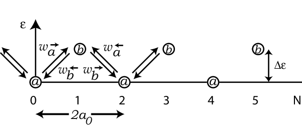
Figure 1: Graphical representation of a simplified lattice model for molecular motors and the relevant rates $w_{a}^{\rightarrow},w_{a}^{\leftarrow},w_{b}^{\rightarrow},w_{b}^{\leftarrow}$ and energy difference $\Delta\varepsilon$. The distinct even and odd sublattices are denoted by $a$ and $b$ respectively.

The rate constants in Eq. 1 define a set of differential equations for the probability $P_{n}(t)$ of being at site $n$ at time $t$. For odd $n$ one has

$$\frac{dP_{n}(t)}{dt}=w_{a}^{\rightarrow}P_{n-1}(t)+w_{a}^{\leftarrow}P_{n+1}(t)-(w_{b}^{\rightarrow}+w_{b}^{\leftarrow})P_{n}(t)\;,$$ (3)

while for even $n$

$$\frac{dP_{n}(t)}{dt}=w_{b}^{\rightarrow}P_{n-1}(t)+w_{b}^{\leftarrow}P_{n+1}(t)-(w_{a}^{\rightarrow}+w_{a}^{\leftarrow})P_{n}(t)\;.$$ (4)

It is illuminating, especially when we consider rate constants which depend on the position along a heterogenous track, to study two limits of these equations. In the first the chemical potential difference $\Delta\mu$ and the applied force $f$ are small compared to the energy difference $\Delta\varepsilon$ so that $b$ states relax quickly compared to $a$ states. This condition implies that $(w_{b}^{\rightarrow}+w_{b}^{\leftarrow})\gg(w_{a}^{\rightarrow}+w_{a}^{\leftarrow})$ so that in the long time-limit to a good approximation the left hand side of Eq. 3 may be set to zero. Upon solving for $P_{n}(t)$ with $n$ odd and substituting into Eq. 4, we obtain differential equations just for the even sites

$$\frac{dP_{n}(t)}{dt} = \frac{w_{b}^{\leftarrow}w_{a}^{\leftarrow}P_{n+2}(t)+w_{b}^{\rightarrow}w_{a}^{\rightarrow}P_{n-2}(t)-(w_{b}^{\rightarrow}w_{a}^{\rightarrow}+w_{b}^{\leftarrow}w_{a}^{\leftarrow})P_{n}(t)}{(w_{b}^{\rightarrow}+w_{b}^{\leftarrow})}\;,$$ (5)

$${\rm(n\;even)}\;.$$

Similarly in the limit $\Delta\mu\gg\Delta\varepsilon$ (with $f$ near the stall force) the motor spends most if its time in $b$ states. Now, in the long time-limit to a good approximation the left hand side of Eq. 4 may be set to zero. The remaining differential equations for the odd sites read

$$\frac{dP_{n}(t)}{dt} = \frac{w_{b}^{\leftarrow}w_{a}^{\leftarrow}P_{n+2}(t)+w_{b}^{\rightarrow}w_{a}^{\rightarrow}P_{n-2}(t)-(w_{b}^{\rightarrow}w_{a}^{\rightarrow}+w_{b}^{\leftarrow}w_{a}^{\leftarrow})P_{n}(t)}{(w_{a}^{\rightarrow}+w_{a}^{\leftarrow})}\;,$$ (6)

$${\rm(n\;odd)}\;.$$

Note that in both limits the dynamics of the motors on long-times can be described by a random walker moving on an effective energy landscape associated with what is in general a non-equilibrium dynamics. Upon absorbing the denominator factors $(w_{a}^{\rightarrow}+w_{a}^{\leftarrow})$ and $(w_{b}^{\rightarrow}+w_{b}^{\leftarrow})$ into a rescaling of the rate constants in the numerator, the effective energy landscape can be read off from Eq. 5 or Eq. 6. One finds that the effective energy difference between two sites which are two monomers apart is given by

$$E_{n+2}-E_{n}\equiv\Delta E=T\ln\left(\frac{w_{a}^{\leftarrow}w_{b}^{\leftarrow}}{w_{a}^{\rightarrow}w_{b}^{\rightarrow}}\right)\;.$$ (7)

For a periodic track, this leads to a tilted energy landscape (with tilt controlled by $\Delta\mu$ and $f$) and an effective energy difference between $2m$-adjacent monomers $2m\Delta E$. The tilted energy landscape leads to diffusion with drift on long time-scales and large length-scales. The effective energy landscape can also be obtained by assuming detailed balance and equating the rate asymmetry between two neighboring even sites to an effective energy difference $\Delta E$. It is straightforward to verify from Eq. 7 with Eq. 1 that for a periodic substrate no net motion is generated when the external force $f=0$ and the chemical potential difference $\Delta\mu=0$. Also, when there is directional symmetry in the transition rates, $\alpha=\alpha^{\prime}$, $\omega=\omega^{\prime}$, and $f=0$ no net motion is generated even when $\Delta\mu\neq 0$. Absent this symmetry, chemical energy can be converted to motion. These conditions are equivalent to those presented in [7, 10] for continuum models and are exhibited here in a minimal model. The effect of the externally applied force is simply to bias the motion of the motor in the direction in which it is applied.

The velocity for a motor moving along a periodic track in the two limits discussed above can be obtained by taking the continuum limit and yields $v=(w_{a}^{\rightarrow}w_{b}^{\rightarrow}-w_{a}^{\leftarrow}w_{b}^{\leftarrow})/(w_{b}^{\rightarrow}+w_{b}^{\leftarrow})$ for the limit specified by Eq. 5 and $v=(w_{a}^{\rightarrow}w_{b}^{\rightarrow}-w_{a}^{\leftarrow}w_{b}^{\leftarrow})/(w_{a}^{\rightarrow}+w_{a}^{\leftarrow})$ for the limit specified by Eq. 6. More generally, for periodic rates, it is straightforward to calcualte the velocity, for example using Bloch eigenfunctions $|k\rangle\sim e^{ikx}$ and expanding the eigenvalues in the wavevector $k$. The linear term gives the velocity and the quadratic part the effective diffusion constant. For the velocity one finds

$$v=\frac{w_{a}^{\rightarrow}w_{b}^{\rightarrow}-w_{a}^{\leftarrow}w_{b}^{\leftarrow}}{w_{a}^{\rightarrow}+w_{b}^{\rightarrow}+w_{a}^{\leftarrow}+w_{b}^{\leftarrow}}\;.$$ (8)

An alternative to studying the solution of the equations, which will be very useful throughout this paper, is to use Monte-Carlo simulations. The rates specified in Eq. (1) can be simulated using the following procedure: To make the simulation efficient we first normalize the entering or leaving rates for a site so that the largest one is unity. Then, at each step we choose with equal probability attempting to move the motor to the right or left on the lattice. Following this choice a random number is drawn from a uniform distribution in the interval $[0,1]$. The motor is moved in the chosen direction provided the random number is smaller than the corresponding rate. Thus, if a motor finds itself on site $a$ in Fig. 1 and $w_{a}^{\rightarrow}>w_{a}^{\leftarrow},w_{b}^{\rightarrow},w_{b}^{\leftarrow}$ is the largest rate it will (after the rescaling) move one step to the right with probability $1/2$, one step to the left with probability $1/2\left(w_{a}^{\leftarrow}/w_{a}^{\rightarrow}\right)$ and it will stay put with probability $1/2[1-(w_{a}^{\leftarrow}/w_{a}^{\rightarrow})]$. Note that the probability of actually moving one step (right or left) to the $b$-sublattice during a particular attempt is $1/2[1+(w_{a}^{\leftarrow}/w_{a}^{\rightarrow})]$. Once the $b$-sublattice is reached the procedure is repeated with the rates $w_{b}^{\rightarrow}$ and $w_{b}^{\leftarrow}$ (note that the probabilities are still obtained by dividing by $w_{a}^{\rightarrow}$). To compare, for example, velocities for different choices of rates the overall number of attempts is rescaled at the end by the fastest rate (taken to be $w_{a}^{\rightarrow}$ in the above example). The same procedure is followed for both homogeneous and heterogeneous tracks. For the latter the largest rate is chosen from all possible hopping rates along the track. This protocol ensures relaxation to equilibrium in the absence of chemical or mechanics driving forces [28].

In [21] we have analyzed in detail the motion of the model when the track is not periodic. Such tracks arise naturally, for example, for motors such as RNA polymerase or helicases which move on DNA which has a well defined sequence. In this case the energy difference $\Delta E(m)$ now becomes an explicit function of the location $m$ along the track, due to the dependance of the rates on the location on the track.

To understand the energy which arises for heterogeneous tracks consider the “integrating out” procedure applied to the three sites shown in Fig. 2, where three distinct motor binding energies, $E_{1}$, $E_{2}$ and $E_{3}$, are indicated explicitly.

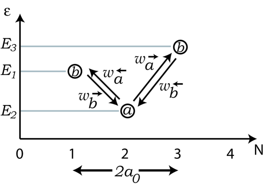
Figure 2: The transition rates and energy levels of three sites, spanning two monomers corresponding to a motor moving along a heterogenous track. Note that $E_{1}\neq E_{3}$ due to the non-periodicity of the track. The transition rates now depend explicitly on the location along the track. To avoid cluttering this dependence was suppressed in the figure.

We work in the limit $\Delta\mu\gg\Delta E$, with $\Delta E=E_{1}-E_{2}$ or $\Delta E=E_{3}-E_{2}$, and $f$ close to the stall force, so that the approximation leading to Eq. 6 (“integrating out” site $2$) is appropriate. As rates for the heterogeneous cluster shown in Fig. 2, we take

$$w_{a}^{\rightarrow}(13) = [\alpha(13)e^{\Delta\mu(13)/T}+\omega(13)]e^{-(E_{2}-E_{1})/T-f/2T}$$

$$w_{b}^{\leftarrow}(13) = [\alpha(13)+\omega(13)]e^{f/2T}$$

$$w_{a}^{\leftarrow}(13) = [\alpha^{\prime}(13)e^{\Delta\mu(13)/T}+\omega^{\prime}(13)]e^{-(E_{2}-E_{3})/T+f/2T}$$ (9)

$$w_{b}^{\rightarrow}(13) = [\alpha^{\prime}(13)+\omega^{\prime}(13)]e^{-f/2T}\;.$$

where the arguments “$(13)$” appended to the $w$’s, $\alpha$’s,$\alpha^{\prime}$’s, $\omega$’s and $\omega^{\prime}$’s simply mean that these are the heterogenous rates appropriate to the cluster $1-2-3$. These rates obey detailed balance conditions for the two channels, and have a similar dependence on $\Delta\mu(13)$ and $f$ and various energy differences as the rates in Eq. 1. The notation $\Delta\mu(13)$ indicates that the chemical potential difference could depend on which NTP (in the case of RNA polymerase) provides the energy for that particular step. Upon assuming fast relaxation of site $2$ in Fig. 2, from a formula similar to Eq. 7,

$$\Delta E_{13} = E_{3}-E_{1}+2f-T\ln\left[\frac{(\alpha(13)e^{\Delta\mu/T}+\omega(13))(\alpha^{\prime}(13)+\omega^{\prime}(13))}{(\alpha^{\prime}(13)e^{\Delta\mu/T}+\omega^{\prime}(13))(\alpha(13)+\omega(13))}\right]\;,$$ (10)

$$\equiv E_{3}-E_{1}+2f+\eta_{13}$$

Eq. 10 illustrates the following important points, applicable to motor molecules on heterogenous tracks more generally: ($a$) if $\Delta\mu(13)=0$, then $E_{13}=E_{3}-E_{1}+2f$, with a similar formula for all neighboring pairs of odd sites. Thus, in the absence of chemical energy, we have a “random energy landscape” with bounded energy fluctuations; ($b$) if $\alpha(13)=\alpha^{\prime}(13)$ and $\omega(13)=\omega^{\prime}(13)$ (inversion symmetry), chemical energy does not lead to net motion between sites $1$ and $3$, as discussed above; ($c$) in general, $\Delta E_{13}=E_{3}-E_{1}+2f+\eta_{13}$, where $\eta_{13}$ is a random function of position along the heterogeneous track. Upon passing to a coarse-grained position $\eta(m)$, where $m$ is the position along the track we see that the effective ‘coarse grained’ energy difference between two points $m_{1}$ and $m_{2}=m_{1}+m$ which are $m$-monomers apart is given by $\sum_{m^{\prime}=m_{1}}^{m_{1}+m}\eta(m^{\prime})$. The landscape itself behaves like a random walk with fluctuations which grow as $\sqrt{m}$, corresponding to a random-forcing energy landscape (for RNA polymerase, the different chemical potentials of the nucleotides in the transcript also contribute to a random forcing landscape [21]).

The self-similar structure of the random force landscape leads to interesting dynamics near the stall force. As the stall force is approached the dynamics slows down and becomes dominated by motion between deep minima of the energy landscape [29]. The minima correspond to specific locations along the track where the motor tends to pause. The distribution of dwell times at these minima, $P(\tau)$, averaged over the different locations on the track, is expected to behave as $\tau^{-(1+\mu)}$, where $\mu$ (not to be confused with a chemical potential!) is related to the force, fluctuations in the effective energy landscape and temperature. For random forcing energy landscape where the energy difference between two points is drawn from a Gaussian distribution with a variance $V=\overline{\eta(m)^{2}}$, where the overline denotes an average along the sequence, one can show that [29]

$$\mu(f)=2T|\overline{\Delta E}_{f=0}-2f|/V\;,$$ (11)

where $\overline{\Delta E}_{f=0}$ is the mean slope of the potential (averaged along the sequence) at zero force. The exponent $\mu$ thus decreases continuously to zero as $f$ increases toward the stall force of the motor (defined by $\mu(f_{s})\equiv 0$). For more general distributions of the effective energy difference the value of $\mu$ might be different from Eq. 11 by factors of order unity.

Near the stall force the expected distribution of pause times becomes broader as $\mu$ becomes closer to $0$. The dynamics of the motors are altered from diffusion with drift when the pause-time distribution becomes very broad. The dynamics then depends on the numerical value of $\mu$ defined in Eq. 11 [21, 22, 29]:

• ${\mu<1}$ – Around the stall force, both the drift and diffusive behavior of the motor become anomalous. The displacement of the motor as a function of time increases as $t^{\mu}$. Thus, in this region the velocity is undefined, in the sense that it depends on the experimental observation time, $t_{E}$, through $v\sim t_{E}^{\mu-1}$. Moreover, the spread of the probability distribution of the motor about its mean position also behaves anomalously with a variance which grows as $t_{E}^{2\mu}$. Experimentally, for a given $t_{E}$, this anomaly should lead to a convex velocity as a function of force curve in the vicinity of the stall force. The curve will become more and more convex as $t_{E}$ is increased; the velocity actually vanishes for a range of $f$’s near the stall force in the limit $t_{E}\to\infty$.

• $1<\mu<2$ – Further away from the stall force the displacement of the motor as a function of time grows linearly. At long-times the velocity becomes independent of the averaging window. However, the variance of the probability distribution around the mean is anomalous and grows as $t_{E}^{2/\mu}$.

• $\mu>2$ – Far below the stall force both the displacement and the variance of the probability distribution around the mean grow linearly in time, as in conventional diffusion with drift.

These results can easily be shown to apply as well to general $n$-state models. Moreover, it can be argued that even if several parallel channels exist for moving from one monomer to another the results are also qualitatively unchanged [21].

Experimentally, the predictions of the model can be tested by measuring the displacement of the motor as a function of time, averaged over different experimental runs (and, possibly, sequences). Each time trace of the motor position will have an irregular shape due to pauses, which will increase in duration as the stall force is approached, at specific locations along the track. However, averaged over many time traces (or sequences) the expected displacement will grows as $t^{\mu}$ with $\mu<1$ close enough to the stall force. Note that if one averages over time traces for a fixed sequence, the displacement is expected to grow as $s(t)t^{\mu}$ where $s(t)$ has fluctuations of order unity, because the sequence information is not completely erased in this case. An alternative experimental test would be to measure the distribution of dwell times ${\cal P}(\tau)$. Because ${\cal P}(\tau)\sim 1/\tau^{1+\mu}$ for large $\tau$, the distribution becomes wider as the stall force is approached. Monitoring ${\cal P}(\tau)$ has the advantage of probing the wide distribution even in regimes which are not very close to the stall force.

We now consider limiting cases of the above model on heterogeneous tracks. These illustrate a number of interesting features and suggest ways in which the anomalous dynamics might be observed experimentally. We will also use the model to explore heterogeneous chemical energy sources for motors on a periodic track. This situation may be realized in motors such as kinesin which can use several types of chemical energy to move along the track. From the two state model described above we deduce the expected behavior of the velocity as the relative proportions of the different fuels is varied and mention generalizations to more general $n$-state models.

3 Strongly biased motors

In this section we study motors moving on a heterogeneous substrate in the limit where one of the transition rates is strongly biased in a certain direction. An extreme limit occurs when one of the transition rates, in, say, the backward direction, is zero. Although this limit violates detailed balance, it could be a reasonable approximation for certain strongly biased experiments. One such model is a special case of the two state model discussed in Section 2:

$$w_{a}^{\rightarrow} = (\alpha e^{\Delta\mu/T}+\omega)e^{-\Delta\varepsilon/T-f/2T}$$

$$w_{b}^{\leftarrow} = (\alpha+\omega)e^{f/2T}$$

$$w_{a}^{\leftarrow} = \omega^{\prime}\;e^{-\Delta\varepsilon/T+f/2T}$$ (12)

$$w_{b}^{\rightarrow} = \omega^{\prime}\;e^{-f/2T}\;.$$

Here we have set $\alpha^{\prime}=0$ so that in the $\Delta\mu\gg T$ limit the motor will be strongly biased to move towards the right. Physically, this situation corresponds to a motor which can use chemical energy only to move in a certain direction. (We expect qualitatively similar results for a wide variety of strongly biased “one way” models). Next, we assume an extremely strong bias $\Delta\mu\gg T$ limit of the model such that $\alpha e^{\Delta\mu/T}$ is very large but $\alpha$ and $\omega$ are so small that $w_{b}^{\leftarrow}$ can be set to be zero. This limit only makes sense far from the stall force. The stall force of a model with $w_{b}^{\leftarrow}=0$ (as any other model were one of the reactions is assumed to be unidirectional) is infinite: The effective energy landscape, Eq. 7, which describes the dynamics of such a limit has an infinite slope. In this section we will compare numerically trajectories when $w_{b}^{\leftarrow}=0$ and when $w_{b}^{\leftarrow}\neq 0$.

Using Eq. 11, the infinite slope of the effective energy landscape implies that $\mu=\infty>2$, so that the dynamics is diffusion with drift. The linear drift is illustrated clearly in Fig. 3 where trajectories of the strongly biased model are shown for different forces. Note that even for very large forces the displacement of the motor as a function of time grows linearly. It can be shown that the dwell time distribution on the track decays exponentially ${\cal P}(\tau)\sim e^{-\tau/\tau^{*}}$ in contrast to the power law distribution expected when $w_{b}^{\leftarrow}\neq 0$. To observe any significant pausing clearly one must have $f\simeq\Delta\mu$ (see inset of Fig. 3). In this limit, however, $w_{a}^{\leftarrow}\gtrsim w_{a}^{\rightarrow}$, and backwards motion cannot be neglected (see Eq. 12).

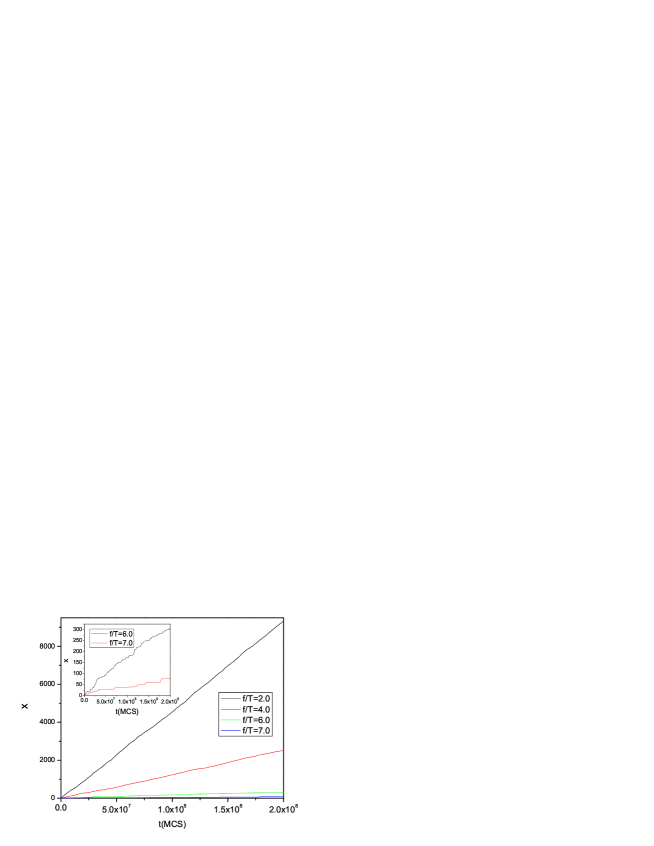
Figure 3: Sample trajectories obtained on a heterogeneous track using the model with $w_{b}^{\leftarrow}=0$ for various values of the reduced force $f/T$. The lower the trajectory the higher the opposing force. Here we took with equal probability $\alpha=5,\omega=1,\omega^{\prime}=2$ and $\alpha=0.2,\omega=1,\omega^{\prime}=1$. In both cases $\Delta\varepsilon=0$ and $e^{\Delta\mu/T}=500$. In the inset the two largest values of the force are presneted in more detail.

In Fig. 4 we show the very different behavior of simulations where we take the back hopping to be non-zero. Now we do not neglect $\omega$ and the backward hopping rate $w_{b}^{\leftarrow}$ is nonzero! For forces near the stall force the displacement of the motor as a function of time seems to saturate even for a trajectory generated by a single numerical experiment for a particular sequence. Such a behavior is consistent with that expected from a sublinear displacement of the motor. Note, however, that with the exception of the largest force, all curves on long enough time scales are expected to yield, after an average over many thermal realizations, an asymptotically linear curve (see the corresponding values of $\mu$ presented in the figure). However, even for these curves, pausing is pronounced despite the fact that for small resisting forces the motor rarely moves backwards.

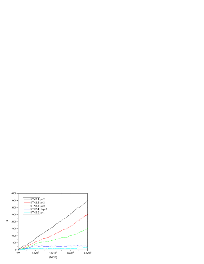
Figure 4: Trajectories obtained using the model of Eq. 12 with $w_{b}^{\leftarrow}=(\alpha+\omega)e^{f/2T}$ and $w_{a}^{\rightarrow}=(\alpha e^{\Delta\mu/T}+\omega)e^{-\Delta\varepsilon/T-f/2T}$. The lower the trajectory the higher the resisting force. Here we took with equal probability $\alpha=5,\omega=1,\omega^{\prime}=2$ and $\alpha=0.2,\omega=1,\omega^{\prime}=1$ along the heterogeneous track. In both cases $\Delta\varepsilon=0$ and $e^{\Delta\mu/T}=500$. Anomalous displacement occur for $f/T>2.47$ while anomalous diffusion occurs for $f/T>2.38$. The stall force is $f_{s}=2.62$.

4 Effect of heterogeneous fuel concentrations for a motor moving along a heterogeneous substrate

For some molecular motors the type of fuel which is used to move depends on the specific site along the track. For example, in the case of RNA polymerase, which produces messenger RNA, the energy from the hydrolysis of the specific NTP which is added to the mRNA chain is used for motion. While a random forcing energy landscape would exist even if the chemical energy released from every NTP were the same (see Sec. 2), the different chemical energies enhance the variance of the slopes, $V$, of the random forcing energy landscape (due to the different chemical potentials of the nucleotides in the transcript). This in turn (see Eq. 11) lowers the value of $\mu$ as compared to the case of equal chemical energies.

As suggested in [21] the variance $V$ could be further increased by increasing the concentration difference between the different NTPs in the solution. In an extreme situation, where one of the NTPs is completely removed from the solution, the motor will stall at specific locations where the NTP is needed. This trick is used in experiments to synchronize and control the motion of RNA polymerases [30]. In this section we illustrate using the simple model, Eq. 1, the effects of changing NTP concentrations on motor motion. Although we work within a “minimal model” we expect the same effects for more complicated models of molecular motors with many internal states (for an example of such a model for RNA polymerase see [31]).

To this end, we studied motors which can use two kinds of fuels depending on its location along the track. We hold the concentration of one fuel fixed and lower the concentration of the other by reducing the chemical potential associated with it. For reference we also study the case when the fuels have equal chemical potentials. Fig. 5 displays results of numerical simulations of the model defined by Eq. (12). Similar results were obtained with the more general model of Eq. (1). We show simulations with $f/T=0$ and when for one fuel $e^{\Delta\mu/T}=500$ and for the other $e^{\Delta\mu/T}=500,50$ or $5$. From a generalization of Eq. 2, we see that this latter variation corresponds to a change of two orders of magnitude in the concentration of the second fuel [14]. As can be seen from Fig. 5, the effect of reducing one of the chemical potentials is to slow down the motion. However, note that for all fuel concentrations the motor displacement as a function of time is linear with these parameter values. Since at zero applied force one expects the motor always to be biased preferentially in a given direction which is independent of the monomer this behavior will hold even for larger differences in concentration.

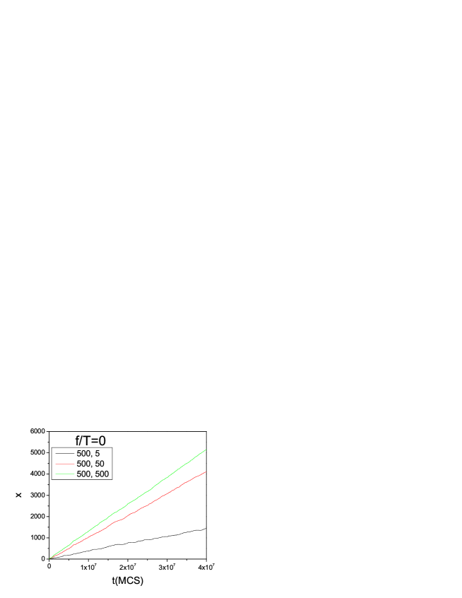
Figure 5: Motor trajectories obtained using the model defined by Eq. (12). Here, substrate heterogeneity is incorporated by taking with equal probability $\{\alpha=5,\omega=1,\omega^{\prime}=2\}$ and $\{\alpha=0.2,\omega=1,\omega^{\prime}=1\}$. The corresponding values of $e^{\Delta\mu/T}$ for the two different fuels are denoted in the box. In both cases $\Delta\varepsilon/T=0$ and $f/T=0$. Lower trajectories correspond to a larger difference in the chemical potentials associated with the fuels.

The change in concentration of one of the fuels can make the regime of anomalous dynamics much larger. In Fig. 6 we show the result of applying a force which opposes the motion of the motors on the dynamics. As can be easily seen from the figure, the velocity of the motors is, of course, lower in comparison to that when no force is applied. However, note that the motion of the curve with the largest difference in chemical potential (barely visible at the bottom) is very different. The motor almost immediately stalls after it starts moving. This example illustrates clearly how changing the concentrations of the different fuels can make the regime of anomalous dynamics easy to access at lower forces. In fact, averaged over many thermal and sequence realizations, the curve with the largest difference in chemical potentials shows a displacement of the motor which grows sublinearly in time, indicating that $\mu<1$.

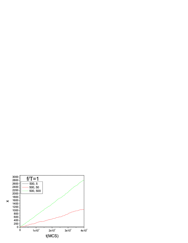
Figure 6: Motor trajectories obtained using the model Eq. (12) with an opposing force. We again took with equal probability $\{\alpha=5,\omega=1,\omega^{\prime}=2\}$ and $\{\alpha=0.2,\omega=1,\omega^{\prime}=1\}$, with the corresponding values of $e^{\Delta\mu/T}$ for the two different fuels as indicated in the figure. In both cases $\Delta\varepsilon/T=0$ and $f/T=1$. Lower trajectories correspond to a larger difference in the chemical potential differences.

5 Heterogeneous fuels on periodic tracks

In this section we consider a molecular motor which is moving along a periodic track in a solution which contains more than one type of molecule which can supply it with chemical energy. The situation arises for kinesin in the presence of both ATP and, say, GTP. It is known that, while less efficient, alternative NTP molecules can also be used by kinesin to move along the track [23, 24, 25]. We consider, for simplicity, a solution with two types of chemical fuels within the simple two state model (The analysis presented can easily be generalized to include additional fuel types). In addition, we generalize our model to treat two separate cases. In the first we assume that the internal states of the motor (i.e., the $a$ and $b$ sites in Fig. 1) are independent of the fuel used so that the chemical fuels are only used to move between states with fuel-dependent potential differences driving the changes. This situation arises when the fuel from the motor is used and released so quickly that the motor is unbound to the fuel in the “excited” internal state. In this case the fuel binding to the motor does not define an internal state. In the second case we study we allow for additional internal states of the motor, depending on which type of chemical fuel is bound to it. This situation arises when internal “excited” states include a fuel bound to the motor. Since the motor bound to the two fuels defines two distinct internal states, a direct thermal transition between them is therefore not possible. While both cases discussed below involve parallel pathways for transitions across a monomer, they are distinct in the type of internal states.

5.1 Case I: Internal states of the motors are independent of the chemical fuel

This case amounts to a straightforward generalization of the rates in Eq. 1 to allow for multiple fuels. As mentioned above, we assume the internal states of the motor are independent of the chemical energy and that chemical energy is only used to assist the transitions. With two different chemical fuels, the generalized rates entering Eqs. 3 and Eq. 4 are now

$$w_{a}^{\rightarrow} = (\alpha_{1}e^{\Delta\mu_{1}/T}+\alpha_{2}e^{\Delta\mu_{2}/T}+\omega)e^{-\Delta\varepsilon/T-f/2T}$$

$$w_{b}^{\leftarrow} = (\alpha_{1}+\alpha_{2}+\omega)e^{f/2T}$$

$$w_{a}^{\leftarrow} = (\alpha_{1}^{\prime}e^{\Delta\mu_{1}/T}+\alpha_{2}^{\prime}e^{\Delta\mu_{2}/T}+\omega^{\prime})e^{-\Delta\varepsilon/T+f/2T}$$ (13)

$$w_{b}^{\rightarrow} = (\alpha_{1}^{\prime}+\alpha_{2}^{\prime}+\omega^{\prime})e^{-f/2T}\;.$$

There are now three parallel paths, two assisted by chemical energy, one thermal. The subscript $1$ or $2$ refers to whether fuel “$1$” or “$2$” is being used for the transition. Standard relations for the chemical potential difference [14] imply that $e^{\Delta\mu_{i}/T}$ grows linearly with the concentration of fuel “$i$” (see Eq. 2). Because the extra channel is present, when one of the chemical potential differences is set to zero the model reduces to the single motor model but with modified rates as compared to a motor in a solution where the fuel is completely absent. For example, if $\Delta\mu_{2}=0$ the model can be written in terms of Eq. 1 with the identifications $\omega\rightarrow\omega+\alpha_{2}$ and $\omega^{\prime}\rightarrow\omega^{\prime}+\alpha^{\prime}_{2}$. Note also that, in contrast to disordered tracks where the motion of the motor is described by a random walker moving on a random force landscape, here the energy landscape is periodic except for a well defined tilt given by Eq. 7.

With the help of Eq. 8, it is straightforward to verify that for this model the velocity takes the form

$$v=\frac{A+B[x_{1}]+B^{\prime}[x_{2}]}{C+D[x_{1}]+D^{\prime}[x_{2}]}\;,$$ (14)

where $[x_{1}]$ and $[x_{2}]$ are the concentrations of fuel $1$ and $2$ respectively and $A,B,B^{\prime},C,D,D^{\prime}$ are complicated functions of the the coefficients in Eq. 13. The velocity thus varies as ratio of two polynomials, each depending linearly on the concentration of both fuels. Consider, for example, the velocity in an experiment where one of the fuels is held at constant concentration and the concentration of the other is varied. The external force is set to $f=0$; (varying $f$ did not affect the qualitative features discussed below). As shown in Fig. 7, the average velocity smoothly crosses over from a small value to a larger value in a sigmoidal fashion as the concentration of more energy rich fuel (“fuel $1$”) is increased. Note that $\Delta\mu_{1}/T$ varies logarithmically with the concentration of fuel number $1$ [14]. Thus, the concentration of fuel “$1$” varies over many orders of magnitude for the range of $\Delta\mu_{1}/T$ shown in Fig. 7. In typical experiments, only a small portion of this crossover may be visible. For small $\Delta\mu_{1}/T$, motor movement is controlled by fuel “$2$” while for large $\Delta\mu_{1}/T$ it is controlled by fuel “$1$”. An analogous plot for motor velocity vs. $\Delta\mu_{1}/T$ when fuel $2$ is absent entirely is shown for reference in Fig. 8. As expected, the velocity no longer exhibits a sigmoidal crossover between two regimes.

Figure 7: The velocity as a function of the chemical potential difference $\Delta\mu_{1}/T$ of fuel “$1$”. The velocity is plotted in units where is size of a monomer (i.e., the lattice constant $2a_{0}$ in Fig. 1) is set to be one and arbitrary time units. We used a “nearly one way model” based on Eq. 13 where the rates were chosen to be $\alpha_{1}=5,\alpha_{2}=2,\alpha_{1}^{\prime}=0.01,\alpha_{2}^{\prime}=0.02,\omega=0.01,\omega^{\prime}=0.2$ in arbitrary units of inverse time and $\Delta\mu_{2}/T=5,f=0,\Delta\varepsilon=0$. For reference the velocity of with only fuel of type “2” with the same value of $\Delta\mu_{2}/T$ is $v=0.195$.

Figure 8: The velocity in arbitrary time units as a function of the chemical potential difference $\Delta\mu_{1}/T$ where the other chemical channel associated with fuel “2” is closed. The velocity is plotted in units where is size of a monomer is set to be one. The rates were chosen to be $\alpha_{1}=5,\alpha_{2}=0,\alpha_{1}^{\prime}=0.01,\alpha_{2}^{\prime}=0.0,\omega=0.01,\omega^{\prime}=0.2,f=0$ in arbitrary units of inverse time and $\Delta\varepsilon=0$.

5.2 Case II: Internal states of the motors are coupled to the chemical fuel

Next, we consider a different model incorporating two fuels. We now assume that the type of fuel molecule used to move the motor determines the entire chemical cycle which leads the motor to move across one monomer. An example might be the $n=2$ motor landscape shown in Fig. 1 where one step (e.g.; $a$ site $\rightarrow$ $b$ site) involves the fuel molecule binding to the motor. In this case the entire sequence of transitions would be dictated by the fuel that is used. Thus, the choice of rates (either in the forward or backward direction) would be dictated by the initial step which is chosen at random, depending on the type of fuel utilized.

Since the state of the motor is directly coupled to the chemical fuel, a pure thermal transition between the states is not possible (unless it involves moving across the monomer through parallel pathways not related to the motor, an effect which is ignored here). The new feature is that the motor can move across a monomer by choosing one of two distinct chemical pathways. This is in contrast to the model defined by Eq. 13 where two distinct chemical pathways exist for passing between the internal states of the motor, but where the transition across the monomer can occur via a mixture different chemical (or thermal) pathways.

An example for such a model, where each fuel is modeled by a distinct channel which is a special case of the two state model defined by (1) is given by:

$$w_{a}^{\rightarrow} = \alpha e^{\Delta\mu_{1}/T-f/2T}$$

$$w_{b}^{\leftarrow} = \alpha e^{f/2T}$$

$$w_{a}^{\leftarrow} = \omega\;e^{f/2T}$$ (15)

$$w_{b}^{\rightarrow} = \omega\;e^{-f/2T}\;,$$

for the first channel and

$$u_{a}^{\rightarrow} = \gamma e^{\Delta\mu_{2}/T-f/2T}$$

$$u_{b}^{\leftarrow} = \gamma e^{f/2T}$$

$$u_{a}^{\leftarrow} = \nu\;e^{f/2T}$$ (16)

$$u_{b}^{\rightarrow} = \nu\;e^{-f/2T}\;.$$

for the second channel. The fuel concentrations enter through the chemical potential differences $\Delta\mu_{1}$ and $\Delta\mu_{2}$ (see Eq. 2). The relative fuel abundances therefore control the ratio of the rates $w_{a}^{\rightarrow}$ and $u_{a}^{\rightarrow}$. The model will be realized physically in a motor which binds a fuel and uses its chemical energy in the transitions $w_{a}^{\rightarrow}$ or $u_{a}^{\rightarrow}$. The transitions $w_{b}^{\rightarrow}$ and $u_{b}^{\rightarrow}$ involve the release of the corresponding fuel. Here for simplicity we have set the energy difference between the states to be zero and neglected parallel thermal channels. We do not expect the qualitative results described below to be affected by such complications.

The velocity of the model can be calculated in a straightforward manner and is found to be

$$v=\frac{(u_{b}^{\rightarrow}+u_{b}^{\leftarrow})(w_{a}^{\rightarrow}w_{b}^{\rightarrow}-w_{a}^{\leftarrow}w_{b}^{\leftarrow})+(w_{b}^{\rightarrow}+w_{b}^{\leftarrow})(u_{a}^{\rightarrow}u_{b}^{\rightarrow}-u_{a}^{\leftarrow}u_{b}^{\leftarrow})}{(u_{b}^{\rightarrow}+u_{b}^{\leftarrow})(w_{b}^{\rightarrow}+w_{b}^{\leftarrow})+(u_{b}^{\rightarrow}+u_{b}^{\leftarrow})(w_{a}^{\rightarrow}+w_{a}^{\leftarrow})+(u_{a}^{\rightarrow}+u_{a}^{\leftarrow})(w_{b}^{\rightarrow}+w_{b}^{\leftarrow})}\;.$$ (17)

Note that as in Case I, the velocity behaves as a ratio of two polynomials which are linear in the $e^{\Delta\mu_{i}/T}$, and hence with each of the fuel concentrations (similar to Eq. 14). Also similar is the fact that the presence of a second channel alters the velocity even when one of the chemical potential difference is zero. Again, due to the presence of the second channel the velocity is lower than that of the motor in the presence of a single fuel. We do not present plots of the resulting velocity as the concentration of one of the fuels is varied since the qualitative features are similar to those presented in the previous subsection.

Finally, we comment that more complicated scenarios (for example, the existence of additional parallel pathways, or more general $n$-state models) might change the explicit dependence on the concentrations of the fuels. However, we expect a general form of a ratio of two polynomials in the concentrations of the fuels even in much more complicated scenarios. Indeed, with a specific experiment in mind and some structural information on the motor one might be able to use such experiments, coupled with an analysis similar to that presented above, to deduce the number of steps in the chemical cycle which depend explicitly on the fuel concentration. For example, we have considered models where the internal states are independent of the chemical fuel and found that the general velocity can be a ratio of polynomials of a degree which is related to the number of steps which depend on the chemical fuel. However, the detailed results were very dependent on the choice of rates made.

Acknowledgments: We are very grateful to D. K. Lubensky for many stimulating conversations and the collaboration which led to references [21] and [22]. We also thank L. Bau, M. D. Wang and K. C. Neuman for useful conversations and J. Gelles and N. Guydosh for interesting us in the problem of different fuels for kinesin on periodic tracks like microtubules. D.R.N was supported by the National Science Foundation through Grant No. DMR-0231631 and the Harvard Materials Research Laboratory via Grant No. DMR-0213805. Y.K was supported by the Human Frontiers Science Program.

^∗ Permanent address: Department of Physics, Technion, Haifa 32000, Israel.

References

- [1] C. Bustamante, Z. Bryant and S. B. Smith, Nature, 42, 423 (2003).
- [2] C. Bustamante, J. C. Macosko, G. J. L. Wuite, Nature Reviews of Molecular Cell Biology, 1, 130 (2000).
- [3] K. Visscher, M. J. Schnitzer and S. M. Block, Nature, 400, 184 (1999).
- [4] R. J. Davenport, G. J. L. Wuite, R. Landick and C. Bustamante, Science 287, 2497 (2000).
- [5] M. D. Wang, M. J. Schnitzer, H. Yin, R. Landick, J. Gelles and S. M. Block, Science, 282, 902 (1998).
- [6] T. T. Perkins, R. V. Dalal, P. G. Mitsis and S. M. Block, Science, 301, 1914 (2003).
- [7] F. Jülicher, A. Ajdari and J. Prost, Rev. Mod. Phys., 69, 1269 (1997).
- [8] A. Ajdari, Europhys. Lett., 31, 69 (1995).
- [9] A. Parmeggiani, F. Julicher, L. Peliti and J. Prost, Europhys. Lett., 56, 603 (2001).
- [10] J. Prost, J.-F. Chauwin, L. Peliti and A. Ajdari, 72, 2652 (1994).
- [11] M. E. Fisher and A. B. Kolomeisky, Proc. Natl. Acad. Sci. USA, 96, 6597 (1999).
- [12] See also A. B. Kolomeisky and M. E. Fisher, Physica A, 279, 1 (2000).
- [13] A. B. Kolomeisky and M. E. Fisher, Biophys. J., 84, 1642 (2003).
- [14] J. Howard, Mechanics of Motor Proteins and the Cytoskeleton, Sinauer, Sunderland (2001).
- [15] W. Hua, E. C. Young, M. L. Fleming, J. Gelles, Nature, 388, 390 (1997).
- [16] T. Ha, I. Rasnik, W. Cheng, H. P. Babcock, G. H. Gauss, T. M. Lohman and S. Chu, Nature, 419, 638 (2002).
- [17] P. R. Bianco, L. R. Brewer, M. Corzett, R. Balhorn, Y. Yeh, S. C. Kowalczykowski, R. J. Baskin, Nature, 409, 374 (2001).
- [18] A. M. van Oijen, P. C. Blainey, D. J. Crampton, C. C. Richardson, T. Ellenberger, and X. Sunney Xie, Science, 301, 1235 (2003).
- [19] T. T. Perkins, R. V. Dalal, P. G. Mitsis, S. M. Block, Nature, 301, 1914 (2003).
- [20] T. Harms amd R. Lipowsky, Phys. Rev. Lett., 79, 2895 (1997).
- [21] Y. Kafri, D. K. Lubensky and D. R. Nelson, Biophys. J., 86, 3373 (2004).
- [22] Y. Kafri, D. K. Lubensky, D. R. Nelson, Phys. Rev. E, 71, 041906 (2005).
- [23] T. Shimizu, K. Furusawa, S. Ohashi, Y. Y. Toyoshima, M. Okuno, F. Malik and R. D. Vale, J. Cell. Biol. 112, 1189 (1991).
- [24] T. M. Kapoor and T. J. Mitchison, Proc. Natl. Acad. Sci. U. S. A., 96, 9106 (1999).
- [25] S. C. Kuo and M. P. Sheetz, Science, 260, 232 (1993).
- [26] C. K. Peng, S. V. Buldyrev, A. L. Goldberger, S. Havlin, F. Sciortino, M. Simons and H. E. Stanley Nature, 356, 168 (1992).
- [27] A. B. Kolomeisky and B. and Widom, J. Stat. Phys. 93, 633 (1998).
- [28] M. E. J. Newman and G. T. Barkema, Monte Carlo Methods in Statistical Physics, (Oxford, 1999).
- [29] For a review of random forcing energy landscapes see J. P. Bouchaud, A. Comtet, A. Georges and P. Le Doussal, Ann. Phys. (N.Y.), 201, 285 (1990).
- [30] H. Matsuzaki, G. A. Kassavetis and E. P. Geiduschek, J. Mol. Biol., 235, 1173 (1994).
- [31] L. Bai, A. Shundrovsky and M.D. Wang, J. Mol. Biol., 344, 335 (2004).