Current-carrying molecules: a real space picture

Abstract

An approach is presented to calculate characteristic current vs voltage curves for isolated molecules without explicit description of leads. The Hamiltonian for current-carrying molecules is defined by making resort to Lagrange multipliers, while the potential drop needed to sustain the current is calculated from the dissipated electrical work. Continuity constraints for steady-state DC current result in non-linear potential profiles across the molecule leading, in the adopted real-space picture, to a suggestive analogy between the molecule and an electrical circuit.

Experiments on single-molecule junctions are challenging, mainly due to the need of contacting a microscopic object, the molecule, with macroscopic leads Reed et al. (1997); Cui et al. (2001); Reichert et al. (2002); Xu and Tao (2003). Theoretical modeling of molecular junctions is difficult Nitzan and Ratner (2003); Datta (2004); Berman and Mukamel (2004); Sai et al. (2005), and again the description of contacts represents a delicate problem. To attack the complex problem of conduction through a molecular junction a strategy is emerging Kosov (2004); Burke et al. (2005) that focuses attention on isolated molecules and describes the intrinsic molecular conductivity in the absence of electrodes. At variance with common approaches that impose a potential bias to the electrodes and then calculate the resulting current Nitzan and Ratner (2003); Datta (2004); Berman and Mukamel (2004); Sai et al. (2005), a steady-state DC current is forced in the isolated molecule by making resort to a Lagrange-multiplier technique Kosov (2004), or by drawing a magnetic flux through the molecule Burke et al. (2005). Whereas the strategy is promising, two main problems remain to be solved: (1) the calculation of the potential drop needed to sustain the current, and (2) the definition of the potential profile in the molecule. Here I demonstrate that the Joule law can be used to calculate the potential drop from the electrical power dissipated on the molecule. Moreover, continuity constraints for steady-state DC current are implemented in polyatomic molecules in terms of multiple Lagrange multipliers that yield to non-linear potential profiles in the molecule. Finally, in the adopted real-space picture, the current flows through chemical bonds rather than through energy levels, leading to a suggestive description of the molecule as an electrical circuit with resistances associated to chemical bonds.

To start with consider a diatomic Hubbard molecule, whose Hamiltonian $H_{0}$ is defined by $U$, $t$, and the difference of on-site energies: $2\Delta=\epsilon_{2}-\epsilon_{1}$. Following Kosov Kosov (2004), a current is forced through the molecule by introducing a Lagrange multiplier, $\lambda$, as follows:

$$H(\lambda)=H_{0}-\lambda\hat{j}$$ (1)

where $c^{\dagger}_{i,\sigma}$ creates an electron with spin $\sigma$ on the $i$-site, and $\hat{j}=-it\sum_{\sigma}(c^{\dagger}_{1\sigma}c_{2\sigma}-H.c.)$ measures the current flowing through the bond. Here and in the following $\hbar$ and the electronic charge are set to 1, and $t$ is taken as the energy unit. The ground state of $H(\lambda)$, $|G(\lambda)\rangle$, carries a finite current, $J=\langle G(\lambda)|\hat{j}|G(\lambda)\rangle$, and the Lagrange multiplier, $\lambda$, is fixed by imposing a predefined $J$ Kosov (2004). Other molecular properties can be calculated as well, and their dependence on $J$ can be investigated Kosov (2004). Just as an example, the bond-order decreases with $J$, and, in systems with inequivalent sites, the on-site charge distribution is equalized by the current flow. These are interesting informations, but characteristic $J(V)$ curves are still needed.

The Lagrange multiplier, $\lambda$, has the dimensions and the meaning of a magnetic flux drawn across the molecule to generate a spatially uniform electric field Kohn (1964); Burke et al. (2005), $E\propto\omega\lambda$, where $\omega$ is the field frequency Kohn (1964). In the limit of static fields, $\omega\rightarrow 0$, both $E$ and $V$ vanish, suggesting that a finite current flows in the molecule at zero bias. This contrasts sharply with the fundamental relation between charge transport and energy dissipation Nitzan (2001); Datta (2004); Burke et al. (2005): a finite $V$ is needed to sustain a current due to dissipative phenomena occurring in the conductor. Specifically, the Joule law relates the potential drop in a conductor to the electrical power spent on the system to sustain the current, $W=VJ$. Since $J$ is known, $V$ can be obtained from a calculation of the dissipated power.

Dissipation is conveniently described in the density matrix formalism using as a basis of the eigenstates $|k\rangle$ of $H(0)$ Mukamel (1995); Boyd (2003). The equilibrium density matrix, $\sigma_{0}$, is a diagonal matrix whose elements are fixed by the Boltzmann distribution. On the same basis $\sigma(\lambda)$ is a non-diagonal matrix corresponding to a non-equilibrium state whose dynamics is governed by: $\dot{\sigma}=-\frac{i}{\hbar}[H,\sigma]+\dot{\sigma}_{R}$, where $\dot{\sigma}_{R}$ accounts for relaxation phenomena, as due to all degrees of freedom not explicitly described by $H$ (e.g. molecular vibrations, or environmental degrees of freedom also including leads) Mukamel (1995); Datta (2004); Nitzan (2001). Diagonal elements of $\dot{\sigma}_{R}$ describe depopulation and are associated with energy dissipation. As for depopulation I adopt a simple phenomenological model with $(\dot{\sigma}_{R})_{kk}=-\sum_{m}\gamma_{km}\sigma_{mm}$, where $\gamma_{km}$ measures the probability of the transition from $k$ to $m$ Mukamel (1995); Boyd (2003). For the sake of simplicity I will consider the low-temperature limit, with $\gamma_{km}=\gamma$ for $k>m$ and $\gamma_{km}=0$ otherwise. The dynamics of off-diagonal elements is governed by depopulation and dephasing effects: $(\dot{\sigma}_{R})_{km}=-\Gamma_{km}\sigma_{km}$, with $\Gamma_{km}=(\gamma_{kk}+\gamma_{mm})/2+\gamma^{\prime}_{km}$, where $\gamma_{kk}=\sum^{\prime}_{m}\gamma_{mk}$, and $\gamma^{\prime}_{km}$ describes dephasing, i.e. the loss of coherence due to elastic scattering Mukamel (1995); Boyd (2003).

The energy dissipated by the system, $Tr{(\dot{\sigma}_{r}H)}$, has two contributions: the first one, $W_{d}=\sum_{k}(\dot{\sigma}_{R})_{kk}$, is always negative and measures the energy that the system dissipates to the bath as the current flows. This term is governed by depopulation, whereas dephasing plays no role. The second term, $W=-\lambda Tr(\dot{\sigma}_{R}\hat{j})$, measures the electric work done on the system to sustain the current: it is this term that enters the Joule law. In non-degenerate systems $\hat{j}$ is an off-diagonal operator, so that only off-diagonal elements of $\dot{\sigma}_{R}$ enter the expression for $W$. Both depopulation and dephasing then contribute to $V$, and hence to the molecular resistance. This is in line with the observation that a current flowing through a molecule implies an organized motion of electrons along a specific direction Buttiker (1985); Nitzan (2001); Datta (2004). Therefore any mechanism of scattering, either anelastic, as described by depopulation, or elastic, as described by dephasing, contributes to the electrical resistance Buttiker (1985); Datta (2004). The unbalance between $W_{d}$ and $W$ is always positive: the molecule heats as current flows. Efficient heat dissipation is fundamental to reach a steady-state regime and to avoid molecular decomposition Nitzan (2001).

Fig. 1 shows the characteristic curves calculated for a diatomic molecule with $\gamma=0.2$ and $\gamma^{\prime}_{km}=0$. In the left panel results are shown for the symmetric, $\Delta=0$, system. As expected, electronic correlations decrease the conductivity. The results in the right panel for an asymmetric system ($\Delta\neq 0$) show instead an increase of the low-voltage conductivity with increasing $U$. This interesting result is related to the minimum excitation gap, and hence the maximum conductance, of the system with $U=2\Delta$.

Figure 1: Characteristic $J(V)$ curves for a two-site system with different $\Delta$ and $U$. The depopulation rate $\gamma$ is set to 0.2, dephasing is neglected.

The asymmetric diatomic molecule represents a minimal model for the Aviram and Ratner rectifier Aviram and Ratner (1974), however the characteristic curves in the right panel of Fig. 1 are symmetric, and do not support rectification. In agreement with recent results, rectification in asymmetric molecules is most probably due to contacts Datta (2004), or to the coupling between electrons and vibrational or conformational degrees degrees of freedom Troisi and Ratner (2002).

Before attacking the more complex problem of polyatomic molecules, it is important to compare the results obtained so far with well known results for the optical conductivity Kohn (1964). If $\Gamma_{km}=\Gamma$, as it occurs, e.g., for systems with large inhomogeneous broadening (the coherent conductance limit Nitzan and Ratner (2003); Nitzan (2001)), the expression for the potential drop is very simple: $V=\lambda\Gamma$. Then, a perturbative expansion of $J$ leads to the following expression for the zero-bias conductivity, $\mathcal{G}_{0}$:

$${\mathcal{G}}_{0}=\frac{2}{\Gamma}\sum_{k}\frac{\langle k|\hat{j}|g\rangle|^{2}}{E_{k}-E_{g}}$$ (2)

where $g$ is the gs of $H(0)$, with energy $E_{g}$, and the sum runs on all excited states. This expression for the DC conductivity coincides with the zero-frequency limit of the optical conductivity Kohn (1964), provided that the frequency, $\omega$, appearing in the denominator of the expression for the optical conductivity in Ref. Kohn (1964) is substituted by $\omega-i\Gamma$. Introducing a complex frequency to account for relaxation is a standard procedure in spectroscopy Boyd (2003), leading to similar effects as the introduction of an exponential switching on of the electromagnetic field Kohn (1964): both phenomena account for the loss of coherence of electrons driven by an EM field and properly suppress the divergence of the optical conductivity due to the build-up of the phase of electrons driven by a static field.

The connection between DC and optical conductivity breaks down in polyatomic molecules. To keep the discussion simple, I will focus attention on linear Hubbard chains. The optical conductivity of Hubbard chains was discussed based on the current operator $\hat{J}=-ie\sum_{i}t_{i}(c^{\dagger}_{i,\sigma}c_{i+1,\sigma}-H.c.)/\hbar$ Maldague (1977). However, this operator measures the average total current and does not apply to DC currents. Specifically, if a term $-\lambda\hat{J}$ is added to the molecular Hamiltonian, a finite average current is forced through the molecule Kosov (2004), but this current does not satisfy basic continuity constraints for steady-state DC current. In fact, to sustain a steady-state DC current one must avoid the build up of electrical charge at atomic sites. Specifically, in linear molecules the continuity constraint imposes that exactly the same amount of current flows through each bond in the molecule. To impose this constraint the current on each single bond must be under control and a Lagrange multiplier must be introduced for each bond, as follows:

$$H(\lambda_{i})=H_{0}-\sum_{i}\lambda_{i}\hat{j}_{i}$$ (3)

where $\hat{j}_{i}=-it_{i}(c^{\dagger}_{i,\sigma}c_{i+1,\sigma}-H.c.)/\hbar$, and the $\lambda_{i}$’s are fixed by imposing $j_{i}=\langle G|\hat{j}_{i}|G\rangle=J$ independent on $i$.

As before, the electrical work done on the molecule is:

$$W=-\sum_{i}\lambda_{i}Tr(\hat{j}_{i}\dot{\sigma}_{R})$$ (4)

that naturally separates into contributions, $W_{i}$, relevant to each bond. The total potential drop across the molecule, $V=W/J$, is then the sum of the potential drops across each bond, $V_{i}=W_{i}/J$, leading in general to non-linear potential profiles. Of course, in the adopted real-space picture the potential profile can only be calculated at atomic positions, and no information can be obtained on the potential profile inside each bond. Therefore, instead of showing the potential profile along the molecule, I prefer to convey the same information in terms of bond-resistances, defined as: $R_{i}=(\partial J/\partial V_{i})^{-1}$.

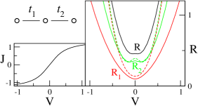
Figure 2: Left panel: characteristic curve for the three-site Hubbard chain sketched in the figure, with 3 electrons, $U=4$, constant on-site energies and $t_{1}=1.2$, $t_{2}=0.8$. Dephasing is set to zero, and depopulation rate is $\gamma=0.1$. Right panel: total resistance ($R$) and bond-resistances ($R_{1}$ and $R_{2}$). For bond-resistances continuous and dashed lines show results obtained by allowing the current to flow through the whole molecule, and through a single bond, respectively.

Fig. 2 shows the behavior of a 3-site chain with three electrons, $U=4$, equal on-site energies and different $t$: $t_{1}=1.2$, and $t_{2}=0.8$. The left panel shows the characteristic $J(V)$ curve, and continuous lines in the right panel report the total resistance $R$, and the two bond resistances, $R_{1}$ and $R_{2}$. The molecular resistance varies with the applied voltage and, as expected, the resistance of the weaker bond is higher than the resistance of the stronger bond.

Dimensionless resistances in the figure are in units with $\hbar/e^{2}=(2\pi\tilde{g}_{0})^{-1}=1$, where $\tilde{g}_{0}$ is the quantum of conductance, that, in standard approaches to molecular junctions Datta (2004) represents the maximum conductance associated with a discrete molecular level. This well known result is related to the inhomogeneous broadening of molecular energy levels as due to their interaction with the electrodes Datta (2004). Of course there is no intrinsic limit to the conductivity in the model for isolated molecules discussed here.

As a direct consequence of the continuity constraint, the total resistance $R=(\partial J/\partial V)^{-1}$ is the sum of the two bond-resistances, leading to a suggestive description of the molecule as an electrical circuit, with resistances associated with chemical bonds joint in series at atomic sites. Whereas this picture is useful, the concept of bond-resistance should be considered with care in molecular circuits. At variance with standard conductors, in fact, the resistance of the bonds depends not only on the circuit (the molecule) they are inserted in, but also on the way the resistance is measured. Dashed lines in Fig. 2 show the bond-resistances calculated by forcing the current through specific bonds (i.e. by setting a single $\lambda_{i}\neq 0$ in Eq. 3), and these differ from the bond-resistances calculated when the whole molecule carries the current (continuous lines).

The situation becomes somewhat simpler in the coherent conductance limit, $\Gamma_{km}=\Gamma$. Perturbative arguments can be used to demonstrate that at zero bias the bond resistances calculated for the current flowing through the whole molecule or through a single bond do coincide. This additive result for the molecular resistance in the coherent transport limit is in line with the observation of transmission rates inversely proportional to the molecular length in the same limit Davis et al. (1997). However, as shown in Fig. 3, this simple Ohmic behavior breaks down quickly at finite bias.

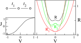
Figure 3: The same as in fig.2, but with $\gamma=0$ and $\gamma^{\prime}_{km}=0.2$.

The introduction of as many Lagrange multipliers as many current-channels (bonds) are present in the molecule accounts for a non-linear potential profile through the molecule, i.e. for a non-uniform electric field. Accounting for a single Lagrange multiplier coupled to the total current operator is equivalent to draw a magnetic flux through the molecule as to generate a spatially homogeneous electric field Kohn (1964); Maldague (1977); Burke et al. (2005), a poor approximation for DC conductivity in extended (polyatomic) molecules. Just as an example, for a 4-site chain with the same $t_{i}=1$ on each bond, the zero-bias resistance of the central bond exceeds that of the lateral bonds with $R_{2}/R_{1}$ ranging from 10 to 2 as $U$ increases from 0 to 4. Bonds with the same $t$ have different resistances due to their different bond-orders, and, in agreement with recent results Liang et al. (2004); Berman and Mukamel (2004), this demonstrates nicely the need of accounting for non-uniform electric fields in extended molecules, even for very idealized molecular structures.

It is of course possible to discuss more complex molecular models. As an interesting example, a nearest-neighbor hopping $t^{\prime}$ is added to the Hamiltonian for the three site molecule discussed above. This opens a new channel for electrical transport, and a term $-\lambda^{\prime}\hat{j}^{\prime}$ adds to the Hamiltonian with $\hat{j}^{\prime}=-it^{\prime}\sum_{\sigma}(c^{\dagger}_{1\sigma}c_{3\sigma}-H.c.)$. As before, continuity imposes $j_{1}=j_{2}$, as to avoid building up of charge at the central site. The total current is $J=j_{1}+j^{\prime}$ and, of course, no continuity constraint is given on $j^{\prime}$. However the potential drop across the molecule, i.e. the potential drop measured at sites 1 and 3 must be uniquely defined. Therefore one must tune $\lambda_{1}$, $\lambda_{2}$ and $\lambda^{\prime}$ as to satisfy $j_{1}=j_{2}$, while satisfying the condition: $V_{1}+V_{2}=V^{\prime}=V$, with $V_{i}=W_{i}/j_{i}$ and $V^{\prime}=W^{\prime}/j^{\prime}$. Imposing a constraint on the potentials is a tricky affair, that becomes trivial when $\Gamma_{km}=\Gamma$.

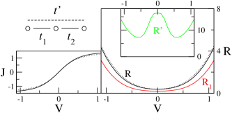
Figure 4: Left panel: characteristic curves of the three site chain sketched in the figure, with three electrons, constant on-site energies, $U=4$, $t_{1}=t_{2}=1$ and $\gamma_{km}=0$ and $\gamma^{\prime}_{km}=0.2$. Continuous and dotted lines refer to $t^{\prime}=0.4$ and 0, respectively. Right panel: molecular and bond-resistances for the chain with $t^{\prime}=0.4$. The dotted line shows the total resistance for the chain with $t^{\prime}=0$.

In that case in fact $V_{i}=\Gamma\lambda_{i}$ and $V^{\prime}=\Gamma\lambda^{\prime}$, so that the constraint on the potentials immediately translates into a constraint on Lagrange multipliers. Fig. 4 shows some results obtained in this limit for a system with $t_{1}=t_{2}=1$, $t^{\prime}=0.4$. In spite of the fairly large $t^{\prime}$ value, the contribution to the current from the bridge-channel is small, mainly due to the small bond-order for next-nearest neighbor sites. Once again the physical constraints imposed to the currents and to the potentials lead to standard combination rules for bond-resistances with $1/R=1/R^{\prime}+1/(R_{1}+R_{2})$. As for the DC conductivity is concerned, the molecule behaves as an electrical circuit with two resistances, $R_{1}$ and $R_{2}$ in series bridged by a parallel resistance, $R^{\prime}$.

Applying the proposed approach to complex molecular structures and/or to molecules described by accurate quantum chemical Hamiltonians is non-trivial due to the appearance in the Hamiltonian of as many Lagrange multipliers as many current channels are considered, and due to the large number of constraints to be implemented. Instead, at least for small molecules, the approach can be fairly easily extended to account for vibrational degrees of freedom. Non-adiabatic calculations are currently in progress to describe electrical conduction through a diatomic molecule in the presence of Holstein and Peierls electron-phonon coupling. More refined models for the relaxation dynamics can also be implemented Davis et al. (1997), whereas the introduction of spin-orbit coupling can lead to a model for spintronics.

In conclusion, this paper presents an approach to the calculation of characteristic current/voltage curves for isolated molecules in the absence of contacts. While hindering the direct comparison with experimental data, this allows the definition of the molecular conductivity as an intrinsic molecular property. Even more important, a paradigm is defined for imposing a steady-state DC current through the molecule, while extracting the voltage drop across the molecule from the energy dissipation. The careful implementation of continuity constraints for steady-state DC current leads to the definition of the potential profile through the molecule, that, in the adopted real-space description, quite naturally results in the concept of bond-resistances, in a suggestive description of the molecule as an electrical circuit with current flowing through chemical bonds.

I thank D. Kosov for useful discussions and correspondence. Discussions with A. Girlando, S. Pati, S. Ramasesha, and Z.G. Soos are gratefully acknowledged. The contributions from S. Cavalca and C. Sissa in the early stages of this work are acknowledged. Work supported by Italian MIUR through FIRB-RBNE01P4JF and PRIN2004033197-002.

References

- Reed et al. (1997) M. A. Reed, C. Zhou, C. J. Muller, T. P. Burgin, and J. M. Tour, Science 278, 252 (1997).
- Cui et al. (2001) X. D. Cui, A. Primak, X. Zarate, J. Tomfohr, O. F. Sankey, A. L. Moore, T. A. Moore, D. Gust, G. Harris, and S. M. Lindsay, Science 294, 571 (2001).
- Reichert et al. (2002) J. Reichert, R. Ochs, D. Beckmann, H. B. Weber, M. Mayor, and H. V. Lohneysen, Phys. Rev. Lett. 88, 176804 (2002).
- Xu and Tao (2003) B. Q. Xu and N. J. Tao, Science 301, 1221 (2003).
- Nitzan and Ratner (2003) A. Nitzan and M. A. Ratner, Science 300, 1384 (2003).
- Datta (2004) S. Datta, Nanotechnology 15, S433 (2004).
- Berman and Mukamel (2004) O. Berman and S. Mukamel, Phys. Rev. B 69, 155430 (2004).
- Sai et al. (2005) N. Sai, M. Zwolak, G. Vignale, and M. D. Ventra, Phys. Rev. Lett. 94, 186810 (2005).
- Kosov (2004) D. S. Kosov, J. Chem. Phys. 120, 7165 (2004).
- Burke et al. (2005) K. Burke, R. Car, and R. Gebauer, Phys. Rev. Lett. 94, 146803 (2005).
- Kohn (1964) W. Kohn, Phys. Rev. 133, A171 (1964).
- Nitzan (2001) A. Nitzan, Ann. Rev. Phys. Chem. 52, 681 (2001).
- Mukamel (1995) S. Mukamel, Principles of Nonlinear Optical Spectroscopy (Oxford Univ. Press, 1995).
- Boyd (2003) R. W. Boyd, Nonlinear Optics (Academic Press, 2003).
- Buttiker (1985) M. Buttiker, Phys. Rev. B 32, 1846 (1985).
- Aviram and Ratner (1974) A. Aviram and M. A. Ratner, Chem. Phys. Lett. 29, 274 (1974).
- Troisi and Ratner (2002) A. Troisi and M. A. Ratner, J. Am. Chem. Soc. 124, 14528 (2002).
- Maldague (1977) P. F. Maldague, Phys. Rev. B 16, 2437 (1977).
- Davis et al. (1997) W. B. Davis, M. R. Wasielewski, M. A. Ratner, V. Mujica, and A. Nitzan, J. Phys. Chem. 101, 6158 (1997).
- Liang et al. (2004) G. C. Liang, A. W. Gosh, M. Paulsson, and S. Datta, Phys. Rev. B 69, 115302 (2004).