Power Law Blinking Quantum Dots: Stochastic and Physical Models

Abstract

We quantify nonergodic and aging behaviors of nanocrystals (or quantum dots) based on stochastic model. Ergodicity breaking is characterized based on time average intensity and time average correlation function, which remain random even in the limit of long measurement time. We argue that certain aspects of nonergodicity can be explained based on a modification of Onsager’s diffusion model of an ion pair escaping neutralization. We explain how diffusion models generate nonergodic behavior, namely a simple mechanism is responsible for the breakdown of the standard assumption of statistical mechanics. Data analysis shows that distributions of on and off intervals in the nanocrystal blinking are almost identical, $\psi_{\pm}(\tau)\propto A_{\pm}\tau^{-(1+\alpha_{\pm})}$ with $A_{+}\approx A_{-}$ and $\alpha_{+}\approx\alpha_{-}=\alpha$ and $\alpha\approx 0.8$. The latter exponent indicates that a simple diffusion model with $\alpha=0.5$ neglecting the electron-hole Coulomb interaction and/or tunneling, is not sufficient.

I Introduction

Single quantum dots when interacting with a continuous wave laser field blink: at random times the dot turns from a state on, in which many photons are emitted to a state off in which no photons are emitted. While stochastic intensity trails are found today in a vast number of single molecule experiments, the dots exhibit statistical behavior which seems unique. In particular, the dots exhibit power law statistics, aging, and ergodicity breaking. While our understanding of the Physical origin of the blinking behavior of the dots is not complete, several physical pictures have emerged in recent years, which explain the blinking in terms of simple Physics. Here we will review a diffusion model which might explain some of the observations made so far. Then we analyze the stochastic properties of the dots, using a stochastic approach. In particular we review the behaviors of the time and ensemble average intensity correlation functions. Usually it is assumed that these two objects are identical in the limit of long times, however this is not the case for the dots.

II Physical Models

A typical fluorescence intensity trace of a CdSe quantum dot, or nanocrystal (NC), overcoated with ZnS (in short, CdSe-ZnS NC) under continuous laser illumination is shown in Fig.

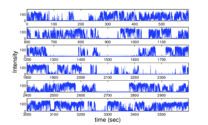
Figure 1: Intensity fluctuations in a CdSe-ZnS NC under continuous laser illumination at room temperature. Dotted horizontal line was selected as a threshold to divide off and on states.

1. From this Figure we learn, that roughly, the intensity jumps between two states - on and off. Some of the deviations from this digital behavior can be attributed to fluctuating non-radiative decay channels due to coupling to the environment, and also to time binning procedure Schlegel et al. (2002); Fisher et al. (2004); Chung and Bawendi (2004), and see also Verberk et al. (2002). Data analysis of such time trace is many times based on distribution of on and off times. Defining a threshold above which the NC is considered in state on and under which it is in state off, one can extract the probability density functions $\psi_{+}(\tau)$ of on and $\psi_{-}(\tau)$ of off times. Surprisingly these show a power-law decay $\psi_{\pm}(\tau)\propto\tau^{-1-\alpha_{\pm}}$, as shown in Fig.

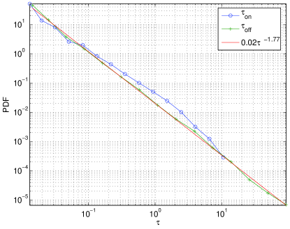
Figure 2: Distributions $\psi_{\pm}(\tau)$ of on and off times for the NC, whose intensity trajectory is shown in Fig. 1. The straight line is the fit to the off time distribution.

2. A summary of different experimental exponents is presented in Table

Group	Material	No.	Radii, nm	Temp., K	Laser Intensity, $\frac{\textrm{kW}}{\textrm{cm}^{2}}$	$\alpha_{+}$	$\alpha_{-}$
Verberk et al. Verberk et al. (2002)	CdS	1	2.5	1.2		$e^{-at}$	0.65(0.2)
Brokmann et al. Brokmann et al. (2003)	CdSe-ZnS	215		300		0.58(0.17)	0.48(0.15)
Shimizu et al. Shimizu et al. (2001)	CdSe-ZnS, CdSe, CdTe	>200	1.5, 2.5	300, 10	0.1-0.7	0.5(0.1), cutoff	0.5(0.1)
Kuno et al. Kuno et al. (2000)	CdSe-ZnS	$\sim 200$	1.7-2.9	300-394	0.24-2.4		0.5-0.75
Kuno et al. Kuno et al. (2001a)	CdSe-ZnS	>300	1.7-2.7	300	0.1-100	0.9(0.05)	0.54(0.03)
Kuno et al. Kuno et al. (2001b)	InP	$\sim 30$	1.5	300	0.24	1.0(0.2)	0.5(0.1)
Cichos et al. Cichos et al. (2004)	Si				1.8, 6.5	1.2(0.1)	0.3, 0.7
Hohng and Ha Hohng and Ha (2004)	CdSe-ZnS	$\sim 1000$					0.94-1.10
Müller et al. Müller et al. (2004)	CdSe-ZnS		4.4 (core)	300	0.025	0.55	0.05, 0.25
van Sark et al. van Sark et al. (2002)	CdSe-ZnS	41	$\sim 3.7$	300	20	$\sim 1.2$, $\sim 0.7$	$\sim 0.2$, $\sim 0.4$
Kobitski et al. Yu. Kobitski et al. (2004)	CdSe		3.6		0.04-0.38	0.97-0.66	0.42-0.64

Table 1: Summary of experimental exponents for on ($\alpha_{+}$) and off ($\alpha_{-}$) time distributions for various single NCs under different experimental conditions. Notice that Verberk et al. use uncapped NCs, while other measurement consider capped NCs, hence exponential distribution on times is found only for uncapped dots. Hohng and Ha used CdSe-ZnS NCs coated with streptavidin which might alter the exponent $\alpha_{-}$.

1, indicating such a power-law decay in most cases. In some cases $\alpha_{+}\approx\alpha_{-}$ and the exponents are close to 1/2. In particular, Brokmann et al. Brokmann et al. (2003) measured 215 CdSe-ZnS NCs and found that all are statistically identical with $\alpha_{+}=0.58\pm 0.17$, $\alpha_{-}\approx 0.48\pm 0.15$ so that $\alpha_{+}\approx\alpha_{-}\approx 0.5$. Note that most of the uncertainty in the values of the exponents can be attributed simply to statistical limitations of data analysis Issac et al. (2005) (see also Section VI below). Shimizu et al. Shimizu et al. (2001) found that in the limit of low temperature and weak laser fields $\alpha_{+}\approx\alpha_{-}\approx 0.5$. The fact that in many cases $\alpha_{\pm}<1$, leads to interesting statistical behavior, for example ergodicity breaking, and aging. We will discuss these behaviors in Sec. III. A physical model for blinking was suggested by Efros and Rosen Efros and Rosen (1997). Briefly the on and off periods correspond to neutral and charged NCs respectively. Thus the on/off trace teaches us something on elementary charging mechanism of the dot. The difficulty is to explain the power law distributions of on and off times, or in other words why should the time the charge occupies the NCs follow power law behavior?

Two types of models were suggested, a diffusion approach and a random trap model. The measurements of Dahan’s and Bawendi’s groups Brokmann et al. (2003); Shimizu et al. (2001), which show the universal power law $\alpha_{\pm}=0.5$, are consistent with the diffusion model (see details below). The fact that all dots are found to be similar Brokmann et al. (2003) seem not consistent with models of quenched disorder Verberk et al. (2002); Kuno et al. (2001a, 2003) since these support the idea of a distribution of $\alpha_{\pm}$. However, some experiments show deviations from the $\alpha_{+}\approx\alpha_{-}\approx 0.5$ and might support the distribution of $\alpha_{\pm}$. It is possible that preparation methods and environments lead to different mechanisms of power law blinking, and different exponents Issac et al. (2005). More experimental work in this direction is needed, in particular, experimentalists still have to investigate the distribution of $\alpha_{\pm}$, and show whether and under what conditions are all the dots statistically identical. Below we discuss the diffusion model; different aspects of the tunneling and trapping model can be found in Verberk et al. (2002); Kuno et al. (2003); Issac et al. (2005).

As discussed at length by Shimizu et al. Shimizu et al. (2001), the on time distributions show temperature and laser power dependencies, e.g. exponential cutoffs of power law behavior. Although no direct observations of cutoffs in the off time distribution was reported, ensemble measurements by Chung and Bawendi Chung and Bawendi (2004) demonstrate that there should be such a cutoff as well, but at times of the order of tens of minutes to hours. Our analysis here, employing the power law decaying distributions, is of course applicable in time windows where power law statistics holds.

II.1 Diffusion model

We note that the simplest diffusion controlled chemical reaction $A+B\rightleftharpoons AB$, where $A$ is fixed in space, can be used to explain some of the observed behavior on the uncapped NCs. As shown by the group of Orrit Verberk et al. (2002) such dots exhibit exponential distribution of on times and power law distribution of off times. The on times follow standard exponential kinetics corresponding to an ionization of a neutral NC (denoted as AB). A model for this exponential behavior was given already in Efros and Rosen (1997). Clearly the experiments of the group of Orrit, show that the capping plays an important part in the the blinking, since capped NCs exhibit power law behavior both for the on and off times. We will return to capped dots later.

Once the uncapped NC is ionized ($A+B$ state) we assume the ejected charge carrier exhibits a random walk on the surface of the NC or in the bulk. This part of the problem is similar to Onsager’s classical problem of an ion pair escaping neutralization (see e.g., Hong and Noolandi (1978); Sano and Tachiya (1979)). The survival probability in the off state for time t, $S_{-}(t)$ is related to the off time distribution via $S_{-}(t)=1-\int_{0}^{t}\psi_{-}(\tau)d\tau$, or

$$\psi_{-}(t)=-\frac{dS_{-}(t)}{dt}.$$ (1)

It is well known that in three dimensions survival probability decays like $t^{-1/2}$, the exponent 1/2 is close to the exponent often measured in the experiments. In infinite domain the decay is not to zero, but the 1/2 appears in many situations, for finite and infinite systems, in completely and partially diffusion controlled recombination, in different dimensions, and can govern the leading behavior of the survival probability for orders of magnitude in time Sano and Tachiya (1979); Nadler and Stein (1991, 1996). In this picture the exponent $1/2$ does not depend on temperature, similar to what is observed in experiment. We note that it is possible that instead of the charge carrier executing the random walk, diffusing lattice defects which serve as a trap for charge carrier are responsible for the blinking behavior of the NCs.

A long time ago, Hong, Noolandi and Street Hong et al. (1981) investigated geminate electron-hole recombination in amorphous semiconductors. In their model they included the effects of tunneling, Coulomb interaction, and diffusion. Combination of tunneling and diffusion leads to a $S(t)\propto t^{-1/2}$ behavior. However, when the Coulomb interactions are included in the theory, deviations from the universal $t^{-1/2}$ law, are observed. For example in the the analysis of photoluminescence decay in amorphous Si:H, as a function of temperature.

Coulomb interaction between the charged NCs and the ejected electron seems to be an important factor in the Physics of NCs. The Onsager radius is a measure of the strength of the interaction

$$r_{Ons}=\frac{e^{2}}{k_{b}T\epsilon}.$$ (2)

Krauss and Brus Krauss and Brus (1999) measured the dielectric constant of CdSe dots, and found the value of $8$. Hence, at room temperature we find $r_{Ons}\simeq 70\textrm{\r{A}}$ (however, note that the dielectric constant of the matrix is not identical to that of the dot). Since the length scale of the dots is of the order of a few nanometers, the Coulomb interaction seems an important ingredient of the problem. This according to the theory in Hong et al. (1981) is an indication of possible deviations from the universal $1/2$ power law behavior. It is also an indication that an ejected electron is likely to return to the dot and not escape to the bulk (since the force is attractive). In contrast, if the Onsager radius is small, an ejected electron would most likely escape to the bulk, leaving the dot in state off forever (i.e. Polya theorem in three dimensions). Unfortunately, currently there is not sufficient experimental data to determine in more qualitative ways if, Onsager type of model can be used to explain the observed data. As in standard geminate recombination processes, the dependence of blinking on temperature, dielectric constant of the dot and of the matrix Issac et al. (2005), and on external driving field, might yield more microscopical information on the precise physical mechanism of the fascinating blinking behavior.

One of the possible physical pictures explaining blinking of capped NCs can be based on diffusion process, using a variation of a three state model of Verberk et al. Verberk et al. (2002). As mentioned above, for this case power law distribution of on and off times are observed. In particular, neutral capped NC will correspond to state on (as for uncapped NCs). However, capped NC can remain on even in the ionized state - see Fig.

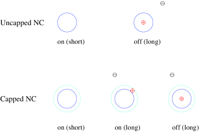
Figure 3: On and off states for NCs, following Verberk et al. (2002).

3. Verberk et al. assume that the ionized capped NC can be found in two states: (i) the charge remaining in the NC can be found in center of NC (possibly a de-localized state), (ii) charge remaining in the NC can be trapped in vicinity of capping. For case (i) the NC will be in state off, for case (ii) the NC will be in state on. Depending on exact location of this charge, the fluorescence intensity can vary. The main idea is that the rate of Auger nonradiative recombination Efros and Rosen (1997) of consecutively formed electron-hole pairs will drop for case (ii) but not for case (i). We note that capping may increase effective radius of the NC, or provide trapping sites for the hole (e.g., recent studies by Lifshitz et al. Lifshitz et al. (2004) demonstrate that coating of NCs creates trapping sites in the interface). Thus the off times occur when the NC is ionized and the hole is close to the center, these off times are slaved to the diffusion of the electron. While on times occur for both a neutral NC and for charged NC with the charge in vicinity of capping, the latter on times are slaved to the diffusion of the electron. In the case of power law off time statistics this model predicts same power law exponent for the on times, because both of them are governed by the return time of the ejected electron.

Beyond nanocrystals, we note that fluorescence of single molecules Haase et al. (2004) and of nanoparticles diffusing through a laser focus Zumofen et al. (2004), switching on and off of vibrational modes of a molecule Bizzarri and Cannistraro (2005), opening-closing behavior of certain single ion channels Nadler and Stein (1991); Goychuk and Hänggi (2002, 2003), motion of bacteria Korobkova et al. (2004), deterministic diffusion in chaotic systems Zumofen and Klafter (1993), the sign of magnetization of spin systems at criticality Godrèche and Luck (2001), and others exhibit power law intermittency behavior Margolin and Barkai (2005a). More generally the time trace of the NCs is similar to the well known Lévy walk model Jung et al. (2002a). Hence the stochastic theory which we consider in the following section is very general. In particular we do not restrict our attention to the exponent 1/2, as there are indications for other values of $\alpha$ between 0 and 1, and the analysis hardly changes.

III Stochastic Model and Definitions

The random process considered in this manuscript, is shown in Fig. 4. The intensity $I(t)$ jumps between two states $I(t)=+1$ and $I(t)=0$. At start of the measurement $t=0$ the NC is in state on: $I(0)=1$. The sojourn time $\tau_{i}$ is an off time if $i$ is even, it is an on time if $i$ is odd (see Fig. 4). The times $\tau_{i}$ for odd [even] $i$, are drawn at random from the probability density function (PDF) $\psi_{+}(t)$, $[\psi_{-}(t)]$, respectively. These sojourn times are mutually independent, identically distributed random variables. Times $t_{i}$ are cumulative times from the process starting point at time zero till the end of the i’th transition. Time $T^{\prime}$ on Fig. 4 is the time of observation. We denote the Laplace transform of $\psi_{\pm}(t)$ using

$$\hat{\psi}_{\pm}(s)=\int_{0}^{\infty}\psi_{\pm}(t)e^{-st}\textrm{d}t.$$ (3)

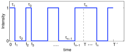
Figure 4: Schematic temporal evolution of the dichotomous intensity process.

In what follows we will investigate statistical properties of this seemingly simple stochastic process. In particular we will investigate the correlation function of this process. In experiment correlation functions are used many times to characterize intensity trajectories. The main advantage of the analysis of correlation functions, if compared with PDFs of on and off times, is that in former case there is no need to introduce the intensity cutoff. Correlations functions are more general than on and off time distributions. Besides, correlation functions exhibit aging, and ergodicity breaking, which are in our opinion interesting.

We will consider several classes of on/off PDFs, and classify generic behaviors based on the small $s$ expansion of $\psi_{\pm}\left(s\right)$. We will consider:
(i) Case 1 PDFs with finite mean on and off times, whose Laplace transform in the limit $s\rightarrow 0$ satisfies:

$$\hat{\psi}_{\pm}(s)=1-s\tau_{\pm}+\cdots.$$ (4)

Here $\tau_{+}$ $(\tau_{-})$ is the average on (off) time. For example exponentially distributed on and off times,

$$\hat{\psi}_{\pm}(s)=\frac{1}{1+s\tau_{\pm}},$$ (5)

belong to this class of PDFs.
(ii) Case 2 PDFs with infinite mean on and off times, namely PDFs with power law behavior satisfying

$$\psi_{\pm}\propto t^{-1-\alpha_{\pm}}\,\,\,\,\,\,\,\,\,\,\,\,\alpha_{-}<\alpha_{+}\leq 1,$$ (6)

in the limit of long times. The small $s$ behavior of these family of functions satisfies

$$\hat{\psi}_{\pm}(s)=1-A_{\pm}s^{\alpha_{\pm}}+\cdots$$ (7)

where $A_{\pm}$ are parameters which have units of time^α. We will also consider cases where on times have finite mean $(\alpha_{+}=1)$ while the off mean time diverges $(\alpha_{-}<1)$ since this situation describes behavior of uncapped NC Verberk et al. (2002) (see also Novikov et al. (2003)).
(iii) Case 3 PDFs with infinite mean with $\alpha_{+}=\alpha_{-}=\alpha$

$$\hat{\psi}_{\pm}(s)=1-A_{\pm}s^{\alpha}+\cdots$$ (8)

As mentioned Brokmann et al. Brokmann et al. (2003) report that for CdSe dots, $\alpha_{+}=0.58\pm 0.17$, and $\alpha_{-}=0.48\pm 0.15$, hence within error of measurement, $\alpha\simeq 0.5$.

Standard theories of data analysis, usually use the ergodic hypothesis and a time average of a process is replaced with an average over an ensemble. The simplest time average in our case is the time average intensity

$$\overline{I}=\frac{\int_{0}^{T^{\prime}}\,\,I(t)\textrm{d}t}{T^{\prime}}.$$ (9)

In the limit of long times and if ergodic assumption holds $\overline{I}=\langle I\rangle$, where $\langle I\rangle$ is the ensemble average. As usual we may generate many intensity trajectories one at a time, to obtain ensemble averaged correlation function

$$C(t,t^{\prime})=\langle I(t)I(t+t^{\prime})\rangle,$$ (10)

and the normalized ensemble averaged correlation function

$$g^{(2)}(t,t^{\prime})\equiv\frac{\langle I(t)I(t+t^{\prime})\rangle}{\left\langle I(t)\right\rangle\left\langle I(t+t^{\prime})\right\rangle}=\frac{C(t,t^{\prime})}{\left\langle I(t)\right\rangle\left\langle I(t+t^{\prime})\right\rangle},$$ (11)

From a single trajectory of $I(t)$, recorded in a time interval $(0,T^{\prime})$, we may construct the time average (TA) correlation function

$$C_{TA}(T^{\prime},t^{\prime})=\frac{\int_{0}^{T^{\prime}-t^{\prime}}I(t)I(t+t^{\prime})\textrm{d}t}{T^{\prime}-t^{\prime}}.$$ (12)

In single molecule experiments, the time averaged correlation function is considered, not the ensemble average. However, it is many times assumed that the ensemble average and the time average correlation functions are identical. For nonergodic processes $C_{TA}(T^{\prime},t^{\prime})\neq C(t,t^{\prime})$ even in the limit of large $t$ and $T^{\prime}$. Moreover for nonergodic processes, even in the limit of $T^{\prime}\rightarrow\infty$, $C_{TA}(T^{\prime},t^{\prime})$ is a random function which varies from one sample of $I(t)$ to another. The ensemble-averaged function $C(t,t^{\prime})$ of the considered process is non-stationary, i.e., it keeps its dependence on $t$ even when $t\rightarrow\infty$. This is known as aging. It follows then from Eq. (12) that $\left\langle C_{TA}(T^{\prime},t^{\prime})\right\rangle=\int_{0}^{T^{\prime}-t^{\prime}}C(t,t^{\prime})dt/(T^{\prime}-t^{\prime})\neq C(t,t^{\prime})$.

IV Aging

Consider the ensemble averaged correlation function $C(t,t^{\prime})=\langle I(t+t^{\prime})I(t)\rangle$. For processes with finite microscopical time scale, which exhibit stationary behavior, one has $C(t,t^{\prime})=f(t^{\prime})$. Namely the correlation function does not depend on the observation time $t$. Aging means that $C(t,t^{\prime})$ depends on both $t$ and $t^{\prime}$ even in the limit when both are large Bouchaud (1992); Aquino et al. (2004). Simple aging behavior means that at the scaling limit $C(t,t^{\prime})=f(t^{\prime}/t)$, which is indeed the scaling in our Case 3; in Case 2 below we find such a scaling for $g^{(2)}(t,t^{\prime})$, while $C(t,t^{\prime})$ will scale differently. Aging and non-ergodicity are related. In our models, when single particle trajectories turn non-ergodic, the ensemble average exhibit aging. Both behaviors are related to the fact that there is no characteristic time scale for the underlying process.

IV.1 Mean Intensity of on-off process

The ensemble averaged intensity $\langle I(t)\rangle$ for the process switching between 1 and 0 and starting at 1 is now considered, which will be used later. In Laplace $t\rightarrow s$ space it is easy to show that

$$\left\langle\hat{I}(s)\right\rangle=\frac{1-\hat{\psi}_{+}(s)}{s}\cdot\frac{1}{1-\hat{\psi}_{+}(s)\hat{\psi}_{-}(s)}.$$ (13)

The Laplace $s\rightarrow t$ inversion of Eq. (13) yields the mean intensity $\langle I(t)\rangle$. Using small $s$ expansions of Eq. (13), we find in the limit of long times

$$\langle I(t)\rangle\sim\left\{\begin{array}[]{cc}\frac{\tau_{+}}{\tau_{+}+\tau_{-}}&\mbox{case}\,\,\,\,1\\ &\\ \frac{A_{+}t^{\alpha_{-}-\alpha_{+}}}{A_{-}\Gamma\left(1+\alpha_{-}-\alpha_{+}\right)}&\mbox{case}\,\,\,\,2\\ &\\ \frac{A_{+}}{A_{+}+A_{-}}&\mbox{case}\,\,\,\,3.\end{array}\right.$$ (14)

If the on times are exponential, as in Eq. (5) then

$$\left\langle\hat{I}(s)\right\rangle=\frac{\tau_{+}}{1+s\tau_{+}-\psi_{-}(s)}.$$ (15)

This case corresponds to the behavior of the uncapped NCs. The expression in Eq. (15), and more generally, the case $\alpha_{-}<\alpha_{+}=1$ leads for long time t to

$$\left\langle I(t)\right\rangle\sim\frac{\tau_{+}t^{\alpha_{-}-1}}{A_{-}\Gamma(\alpha_{-})}.$$ (16)

For exponential on and off time distributions Eq. (5), we obtain the exact solution

$$\left\langle I(t)\right\rangle=\frac{\tau_{-}\exp\left[-t\left(\frac{1}{\tau_{-}}+\frac{1}{\tau_{+}}\right)\right]+\tau_{+}}{\tau_{-}+\tau_{+}}.$$ (17)

The average intensity does not yield direct evidence for aging, because it depends only on one time variable, and one has to consider a correlation function to explore aging in its usual meaning.

Remark For the case $\alpha_{+}<\alpha_{-}<1$, corresponding to a situation where on times are in statistical sense much longer then off times, $\langle I(t)\rangle\sim 1$.

IV.2 Aging Correlation Function of on-off process

The ensemble averaged correlation function $C(t,t^{\prime})=\langle I(t)I(t+t^{\prime})\rangle$ was calculated in Margolin and Barkai (2004). Contributions to the correlation function arise only from trajectories with $I(t)=1$ and $I(t+t^{\prime})=1$, yielding

$$\hat{C}(t,u)=\frac{\hat{f}_{t}(u=0,+)-\hat{f}_{t}(u,+)}{u}$$

$$+\hat{f}_{t}(u,+)\frac{\hat{\psi}_{-}(u)\left[1-\hat{\psi}_{+}(u)\right]}{u\left[1-\hat{\psi}_{-}(u)\hat{\psi}_{+}(u)\right]},$$ (18)

where $u$ is the Laplace conjugate of $t^{\prime}$ and

$$\hat{f}_{s}(u,+)=\frac{\hat{\psi}_{+}(s)-\hat{\psi}_{+}(u)}{(u-s)\left[1-\hat{\psi}_{+}(s)\hat{\psi}_{-}(s)\right]},$$ (19)

where $s$ is the Laplace conjugate of $t$. We note that $\hat{f}_{s}(u,+)$ is the double Laplace transform of the PDF of the so called forward recurrence time. This means that after the aging of the process in time interval $t$, the statistics of first jump event after time $t$ will generally depend on the age $t$. However, a process is said to exhibit aging, only if the statistics of this first jump depend on $t$ even when this age is long. In particular if the microscopical time scale of the problem is infinite, no matter how big is $t$ the correlation function still depends on the age (see details below). The first term in Eq. (18) is due to trajectories which were in state on at time $t$ and did not make any transitions (i.e. the concept of persistence), while the second term includes all the contributions from the trajectories being in state on at time $t$ and making an even number of transitions Margolin and Barkai (2004).

IV.3 Case 1

For case $1$ with finite $\tau_{+}$ and $\tau_{-}$, and in the limit of long times $t$, we find

$$\lim_{t\rightarrow\infty}\hat{C}(t,u)=$$

$$\frac{1}{u}\frac{\tau_{+}}{\tau_{+}+\tau_{-}}\left\{1-\frac{\left[1-\hat{\psi}_{+}(u)\right]\left[1-\hat{\psi}_{-}(u)\right]}{\tau_{+}u\left[1-\hat{\psi}_{-}(u)\hat{\psi}_{+}(u)\right]}\right\}$$ (20)

This result was obtained by Verberk and Orrit Verberk and Orrit (2003) and it is seen that the correlation function depends asymptotically only on $t^{\prime}$ (since u is Laplace pair of $t^{\prime}$). Namely, when average on and off times are finite the system does not exhibit aging. If both $\psi_{+}(t)$ and $\psi_{-}(t)$ are exponential then the exact result is

$$\begin{array}[]{ccc}C(t,t^{\prime})&=&{\displaystyle\frac{\tau_{-}\exp\left[-t\left(\frac{1}{\tau_{-}}+\frac{1}{\tau_{+}}\right)\right]+\tau_{+}}{\tau_{-}+\tau_{+}}}\\ \\ &\times&{\displaystyle\frac{\tau_{-}\exp\left[-t^{\prime}\left(\frac{1}{\tau_{-}}+\frac{1}{\tau_{+}}\right)\right]+\tau_{+}}{\tau_{-}+\tau_{+}}}\end{array}$$

and $C(t,t^{\prime})$ becomes independent of t exponentially fast as t grows.

IV.4 Case 2

We consider case $2$, however limit our discussion to the case $\alpha_{+}=1$ and $\alpha_{-}<1$. As mentioned this case corresponds to uncapped NCs where on times are exponentially distributed, while off times are described by power law statistics. Using the exact solution Eq. (18) we find asymptotically, when both t and $t^{\prime}$ are large:

$$C(t,t^{\prime})\sim\left(\frac{\tau_{+}}{A_{-}}\right)^{2}\frac{\left(tt^{\prime}\right)^{\alpha_{-}-1}}{\Gamma^{2}\left(\alpha_{-}\right)}.$$ (21)

Unlike case $1$ the correlation function approaches zero when $t\rightarrow\infty$, since when $t$ is large we expect to find the process in state off. Using Eq. (16), the asymptotic behavior of the normalized correlation function Eq. (11) is

$$g^{(2)}(t,t^{\prime})\sim\left(1+\frac{t}{t^{\prime}}\right)^{1-\alpha_{-}}.$$ (22)

We see that the correlation functions Eqs. (21, 22) exhibit aging, since they depend on the age of the process $t$.

Considering the asymptotic behavior of $C(t,t^{\prime})$ for large t,

$$\hat{C}(t,u)\approx$$

$$\frac{1}{u}\frac{\tau_{+}}{A_{-}\Gamma(\alpha_{-})t^{1-\alpha_{-}}}\left\{1-\frac{\left[1-\hat{\psi}_{+}(u)\right]\left[1-\hat{\psi}_{-}(u)\right]}{\tau_{+}u\left[1-\hat{\psi}_{-}(u)\hat{\psi}_{+}(u)\right]}\right\}.$$ (23)

This equation is similar to Eq. (20), especially if we notice that the “effective mean” time of state off until total time t scales as $A_{-}t^{1-\alpha_{-}}$.

For the special case, where on times are exponentially distributed, the correlation function C is a product of two identical expressions for all t and $t^{\prime}$:

$$\hat{C}(s,u)=\frac{\tau_{+}}{1+s\tau_{+}-\psi_{-}(s)}\cdot\frac{\tau_{+}}{1+u\tau_{+}-\psi_{-}(u)},$$ (24)

where s (u) is the Laplace conjugate of t ($t^{\prime}$) respectively. Comparing to Eq. (15) we obtain

$$C(t,t^{\prime})=\langle I(t)\rangle\langle I(t^{\prime})\rangle,$$ (25)

and for the normalized correlation function

$$g^{(2)}(t,t^{\prime})=\frac{\left\langle I(t^{\prime})\right\rangle}{\left\langle I(t+t^{\prime})\right\rangle}.$$ (26)

Eqs. (26, 25) are important since they show that measurement of mean intensity $\langle I(t)\rangle$ yields the correlation functions, for this case. While our derivation of Eqs. (26, 25) is based on the assumption of exponential on times, it is valid more generally for any $\psi_{+}(t)$ with finite moments, in the asymptotic limit of large $t$ and $t^{\prime}$. To see this note that Eqs. (21, 16) yield $C(t,t^{\prime})\sim\langle I(t)\rangle\left\langle I(t^{\prime})\right\rangle$.

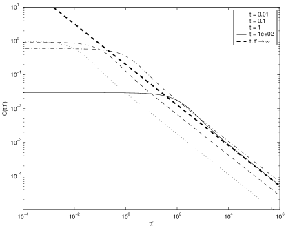
Figure 5: Exact $C(t,t^{\prime})$ for Case $2$: exponential on times and power law off times with $\alpha_{-}=0.4$. We use $\hat{\psi}_{+}(s)=1/(1+s)$ and $\hat{\psi}_{-}(s)=1/(1+s^{0.4})$ and numerically obtain the correlation function. For each curve in the figure we fix the time $t$. The process starts in the state $on$. Thick dashed straight line shows the asymptotic behavior Eq. (21). For short times ($t^{\prime}<1$ for our example) we observe the behavior $C(t,t^{\prime})\sim C(t,0)=\langle I(t)\rangle$, the correlation function is flat.

In Fig. 5 we compare the asymptotic result (21) with exact numerical double Laplace inversion of the correlation function. We use exponential PDF of on times $\psi_{+}(s)=1/(1+s)$, and power law distributed off times: $\hat{\psi}_{-}(s)=\hat{\psi}_{-}(s)=1/(1+s^{0.4})$ corresponding to $\alpha_{-}=0.4$. Convergence to asymptotic behavior is observed.

Remark For fixed $t$ the correlation function in Eq. (21) exhibits a $(t^{\prime})^{\alpha_{-}-1}$ decay. A $(t^{\prime})^{\alpha_{-}-1}$ decay of an intensity correlation function was reported in experiments of Orrit’s group Verberk et al. (2002) for uncapped NCs (for that case $\alpha_{-}=0.65\pm 0.2$). However, the measured correlation function is a time averaged correlation function Eq. (12) obtained from a single trajectory. In that case the correlation function is independent of $t$, and hence no comparison between theory and experiment can be made yet.

IV.5 Case 3

We now consider case $3$, and find Margolin and Barkai (2004)

$$C(t,t^{\prime})=P_{+}-P_{+}P_{-}\frac{\sin\pi\alpha}{\pi}B\left(\frac{1}{1+t/t^{\prime}};1-\alpha,\alpha\right),$$ (27)

where

$$P_{\pm}=\frac{A_{\pm}}{A_{+}+A_{-}}$$

following from Eq. (14), and where

$$B(z;a,b)=\int_{0}^{z}x^{a-1}(1-x)^{b-1}dx$$

is the incomplete beta function. The behavior in this limit does not depend on the detailed shape of the PDFs of the on and off times, besides the parameters $A_{+}/A_{-}$ and $\alpha$. We note that both terms of Eq. (18) contribute to Eq. (27). The appearance of the incomplete beta function in Eq. (27) is related to the concept of persistence. The probability of not switching from state on to state off in a time interval $(t,t+t^{\prime})$, assuming the process is in state on at time $t$, is called the persistence probability. In the scaling limit this probability is

$$P_{0}(t,t+t^{\prime})\sim 1-\frac{\sin\pi\alpha}{\pi}B\left(\frac{1}{1+t/t^{\prime}};1-\alpha,\alpha\right).$$ (28)

The persistence implies that long time intervals in which the process does not jump between states on and off, control the asymptotic behavior of the correlation function. The factor $P_{+}$, which is controlled by the amplitude ratio $A_{+}/A_{-}$, determines the expected short and long time $t^{\prime}$ behaviors of the correlation function, namely $C(\infty,0)=\lim_{t\rightarrow\infty}\langle I(t)I(t+0)\rangle=P_{+}$ and $C(\infty,\infty)=\lim_{t\rightarrow\infty}\langle I(t)I(t+\infty)\rangle=(P_{+})^{2}$. With slightly more details the two limiting behaviors are:

$$C(t,t^{\prime})\sim\left\{\begin{array}[]{cc}P_{+}&\,\,\,\frac{t^{\prime}}{t}\ll 1\\ &\\ (P_{+})^{2}+P_{+}P_{-}\frac{\sin(\pi\alpha)}{\pi\alpha}\left(\frac{t^{\prime}}{t}\right)^{-\alpha}&\,\,\,\frac{t^{\prime}}{t}\gg 1.\end{array}\right.$$ (29)

Using Eq. (14) the normalized intensity correlation function is $g^{(2)}(t,t^{\prime})\sim C(t,t^{\prime})/(P_{+})^{2}$.

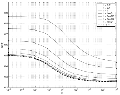
Figure 6: Exact $C(t,t^{\prime})$ for case $3$, when both on and off times are power law distributed with $\alpha=0.4$. We use $\hat{\psi}_{\pm}(s)=1/(1+s^{0.4})$ for different times t increasing from the topmost to the lowermost curves. The dots on the left and on the right show $C(t,0)=\left\langle I(t)\right\rangle$ and $C(t,\infty)=\left\langle I(t)\right\rangle/2$ respectively. The process starts in the state on.

In Fig. 6 we compare the asymptotic result (27) with exact numerical double Laplace inversion of the correlation function for PDFs $\hat{\psi}_{+}(s)=\hat{\psi}_{-}(s)=1/(1+s^{0.4})$. Convergence to Eq. (27) is seen.

Remark For small $t^{\prime}/t$ we get flat correlation functions. Flat correlation functions were observed by Dahan’s group Messin et al. (2001) for capped NCs. However, the measured correlation function is a single trajectory correlation function Eq. (12), and hence no comparison between theory and experiment can be made yet.

V Non Ergodicity

Non-ergodicity of blinking quantum dots was first pointed out in the experiments of the group of Dahan Messin et al. (2001). We begin the discussion of nonergodicity in blinking NCs by plotting 100 time averaged correlation functions from 100 NCs in Fig.

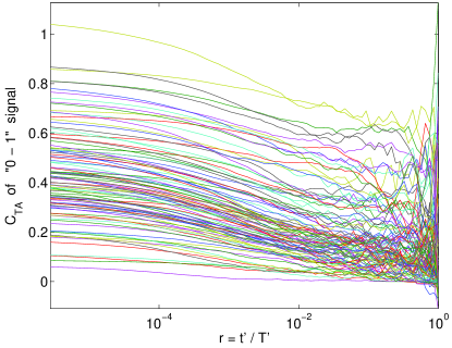
Figure 7: 100 experimental time averaged correlation functions (one of which is obtained from the signal shown in Fig. 1), after “renormalizing” the average on and off intensities to be 1 and 0, respectively. Note logarithmic abscissa.

7. Clearly, correlation functions obtained are different. The simplest explanation would be that the NCs have different statistical properties. However, similar variability is also observed for a given NC, when we calculate correlation functions for different $T^{\prime}$ (e.g., Messin et al. (2001)). To further illustrate this point, we generate on a computer the two state process, with power law waiting time of on and off times following $\psi_{-}(\tau)=\psi_{+}(\tau)=\alpha\tau^{-1-\alpha}$ for $\tau>1$ (and zero otherwise). For each trajectory we calculate its own time average correlation. As we show in Fig.

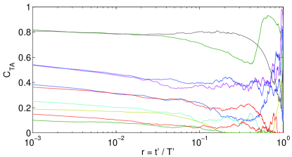
Figure 8: Ten typical simulated realizations of $C_{TA}$ for $\alpha=0.8$.

8 the trajectories exhibit ergodicity breaking. The most striking feature of the figure is that even though trajectories are statistically identical, the correlation function of the process is random, similar to the experimental observation. In complete contrast, if we consider a two state process with on and off times following exponential statistics, then all the correlation functions would be identical, and all of them would follow the same master curve: the ensemble average correlation function.

In this section we consider the non-ergodic properties of the blinking NCs using a stochastic approach. We assume that all the NCs are statistically identical in agreement with Brokmann et al. (2003), and restrict ourselves to the Case 3. For the sake of simplicity we only consider the case when distribution of on times is identical to distribution of off times, namely $\alpha_{-}=\alpha_{+}=\alpha$ and $A_{+}=A_{-}=A$. Generalization to $A_{+}\neq A_{-}$ is straightforward Bel and Barkai (2005). The nonergodicity is found only for $\alpha<1$, when the mean transition time is infinite, and should therefore disappear when exponential cutoffs of off and on times become relevant Chung and Bawendi (2004), i.e., when the mean transition times become of the order, or less than the experimental time. The described model, however, is valid in a wide time window spanning many orders of magnitude for the NCs, and is relevant to other systems, as mentioned in Section II.

V.1 Distribution of time averaged intensity

As mentioned in the introduction, the blinking NCs exhibit a non-ergodic behavior. In particular the ensemble average intensity $\langle I\rangle$ is not equal to the time average $\overline{I}$. Of course in the ergodic phase, namely when both the mean on and off times are finite, we have $\langle I\rangle=\overline{I}$, in the limit of long measurement time. More generally we may think about $\overline{I}$ as a random function of time, which will vary from one measurement to another. In the ergodic phase, and in the asymptotic limit the distribution of $\overline{I}$ approaches a delta function

$$P(\overline{I})\rightarrow\delta(\overline{I}-\langle I\rangle).$$ (30)

The theory of non-ergodic processes deals with the question what is the distribution of $P(\overline{I})$ in the non-ergodic phase. For the two state stochastic model

$$\overline{I}=\frac{T^{+}}{T}$$ (31)

where $T^{+}$ is the total time spent in state on.

A well known example of similar ergodicity breaking is regular diffusion, or a binomial random walk on a line. The walker starts at the origin and can go left or right randomly, at each step. Let the measurement time be $t$, and the position of the random walker be $x(t)$. The total time the walker remains on the right of the origin $x(t)>0$ is $T^{+}$. The PDF of return time (or of number of steps) $\tau$ to the origin decays as $\tau^{-3/2}$ for large $\tau$, so that $\alpha=1/2$. Two half-axes at both sides of the origin can be thought of as the two states, on and off, of the random walker. The well-established result is that the fraction $\overline{I}$ of total time spent by the walker on either side, in the long time limit is given by the arcsine law Feller (1966); Godrèche and Luck (2001)

$$P\left(\overline{I}\right)=\frac{1}{\pi\sqrt{\overline{I}(1-\overline{I})}}.$$

A main feature of this PDF is its divergence at $\overline{I}=0,\,1$, indicating that the random walker will most probably spend most of its time on one side (either left or right) of the origin. In particular the naive expectation that the particle will spend half of its time on the right and half on the left, in the limit of long measurement time, is wrong. In fact the minimum of the arcsine PDF is on $\overline{I}=\langle\overline{I}\rangle=1/2$. In other words the ensemble average $\langle\overline{I}\rangle=1/2$ is the least likely event. This result might seem counter intuitive at first, but it is due to the fact that the mean time for return to the origin is infinite. This in turn means that the particle gets randomly stuck on $x<0$ or on $x>0$ for a period which is of the order of the measurement time, no matter how long this measurement time is.

In the more general case $0<\alpha<1$ the distribution of $\overline{I}$ can be calculated based on the work of Lamperti Lamperti (1958) (see also Godrèche and Luck (2001)), and one finds

$$l_{\alpha}(\overline{I})=\frac{\sin\left(\pi\alpha\right)}{\pi}\frac{\overline{I}^{\alpha-1}\left(1-\overline{I}\right)^{\alpha-1}}{\overline{I}^{2\alpha}+\left(1-\overline{I}\right)^{2\alpha}+2\cos\left(\pi\alpha\right)\overline{I}^{\alpha}\left(1-\overline{I}\right)^{\alpha}},$$ (32)

which is shown in Fig.

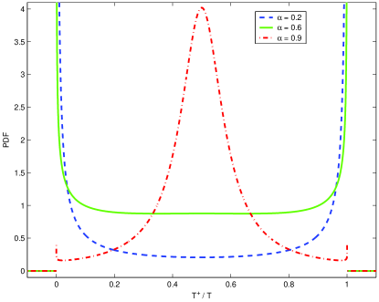
Figure 9: The probability density function of $\overline{I}=T^{+}/T$ for the case $\psi_{+}(t)=\psi_{-}(t)\propto t^{-(1+\alpha)}$. For the ergodic phase $\alpha>1$ $P(\overline{I})$ is a delta function on $\langle I\rangle=1/2$. In the non-ergodic phase $\overline{I}$ is a random function, for small values of $\alpha$ the $P(\overline{I})$ is peaked on $\overline{I}=0$ and $\overline{I}=1$, indicating a trajectory which is in state off or on for a period which is of the order of measurement time $T$.

9. When $\alpha\rightarrow 0$ the PDF of $\overline{I}$ is peaked around $\overline{I}=0$ and $\overline{I}=1$, corresponding to blinking trajectories which for most of the observation time $T$ are in state off or state on respectively. When $\alpha\rightarrow 1$, we see that $l_{\alpha}(\overline{I})$ attains a maximum when $\overline{I}=\langle I\rangle=1/2$, indeed in the ergodic phase $\alpha>1$ we obtain as expected a delta peak centered on $\overline{I}=1/2$, as we mentioned. There exists a critical $\alpha_{c}=0.594611...$ above (under) which $l_{\alpha}(\overline{I})$ has a maximum (minimum) on $\overline{I}=1/2$. Note that the Lamperti PDF in Eq. (32) is not sensitive to the precise shapes of the on and off time distributions (besides $\alpha$ of course). For situations in which $A_{-}\neq A_{+}$ the symmetry of the Lamperti PDF will not hold. Note that line shapes with structures similar to those in Fig. 9, were obtained by Jung et al. Jung et al. (2002b) in a related problem. Similar expressions are also used in stochastic models of spin dynamics Baldassarri et al. (1999), and in general, the problem of occupation times, and a related persistence concept, are of a wide interest in different fields Dhar and Majumdar (1999); Majumdar (2004); Bel and Barkai (2005).

Next we extend our understanding of the distribution of time averaged intensity to the time averaged correlation functions defined in Eq. (12).

V.2 Distribution of time averaged correlation function

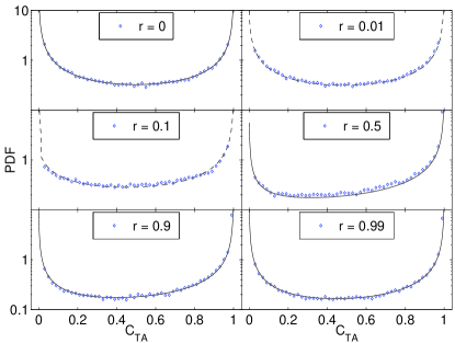
Figure 10: PDF of $C_{TA}(T^{\prime},t^{\prime})$ for different $r=t^{\prime}/T^{\prime}$ and $\alpha=0.3$. Abscissas are possible values of $C_{TA}(T^{\prime},t^{\prime})$. Diamonds are numerical simulations. Curves are analytical results without fitting: for $r=0$ Eq. (32) is used (full line), for $r=0.01$ and 0.1 Eq. (35) is used (dashed) and for $r=0.5$, 0.9 and 0.99 Eq. (38) is used (full).

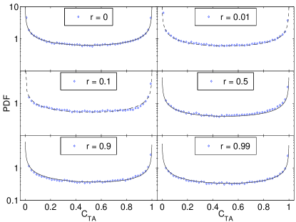
Figure 11: PDF of $C_{TA}(T^{\prime},t^{\prime})$ for different $r=t^{\prime}/T^{\prime}$ and $\alpha=0.5$. Diamonds are numerical simulations. Curves are analytical results without fitting: for $r=0$ Eq. (32) is used (full line), for $r=0.01$ and 0.1 Eq. (35) is used (dashed) and for $r=0.5$, 0.9 and 0.99 Eq. (38) is used (full).

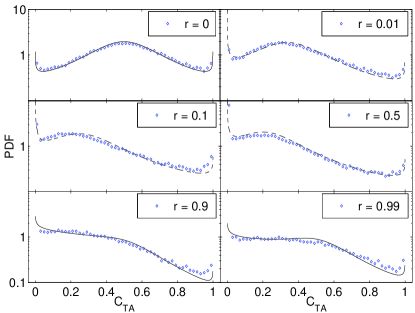
Figure 12: PDF of $C_{TA}(T^{\prime},t^{\prime})$ for different $r=t^{\prime}/T^{\prime}$ and $\alpha=0.8$. Diamonds are numerical simulations. Curves are analytical results without fitting: for $r=0$ Eq. (32) is used (full line), for $r=0.01$, 0.1 and 0.5 Eq. (35) is used (dashed) and for $r=0.9$ and 0.99 Eq. (38) is used (full). If compared with the cases $\alpha=0.3$ and 0.5, the distribution function exhibits a weaker non-ergodic behavior, namely for $r=0$ the distribution function peaks on the ensemble average value of $1/2$.

We first consider the non-ergodic properties of the correlation function for the case $t^{\prime}=0$. It is useful to define

$$\mathcal{I}_{[a,b]}=\int_{a}^{b}I(t)\textrm{d}t/(b-a),$$ (33)

the time average intensity between time $a$ and time $b>a$, and

$$T=T^{\prime}-t^{\prime},$$

$$r=\frac{t^{\prime}}{T^{\prime}}.$$

Using Eq. (12) and for $t^{\prime}=0$ the time averaged correlation function is identical to the time average intensity

$$C_{TA}(T,0)=\mathcal{I}_{[0,T]}=\frac{T^{+}}{T},$$ (34)

and its PDF is given by Eq. (32). Figs. 10, 11 and 12 for the case $r=0$, show these distributions for $\alpha=0.3$, 0.5 and 0.8, respectively, together with the numerical results.

An analytical approach to estimate the distributions $P_{C_{TA}(T^{\prime},t^{\prime})}(z)$ of $C_{TA}(T^{\prime},t^{\prime})=z$ for nonzero $t^{\prime}$ was developed in Margolin and Barkai (2005a); Margolin and Barkai (2005b). To treat the problem a non-ergodic mean field approximation was used, in which various time averages were replaced by the time average intensity $\mathcal{I}_{[0,T]}$, specific for a given realization. For short $t^{\prime}\ll T^{\prime}$ the result is

$$C_{TA}(T^{\prime},t^{\prime})\simeq\left\{\begin{array}[]{l l}{\mathcal{I}}_{[0,T]}\left\{1-\left(1-{\mathcal{I}}_{[0,T]}\right)\left[\left({r\over{(1-r)\mathcal{I}}_{[0,T]}}\right)^{1-\alpha}\left({\sin\pi\alpha\over\pi\alpha}+1\right)-{\sin\pi\alpha\over\pi\alpha}{r\over{(1-r)\mathcal{I}}_{[0,T]}}\right]\right\}&\ t^{\prime}<T^{+}\\ {\mathcal{I}}_{[0,T]}^{2}&\ t^{\prime}>T^{+}.\end{array}\right.$$ (35)

Eq. (35) yields the correlation function, however unlike standard ergodic theories the correlation function here is a random function since it depends on $\mathcal{I}_{[0,T]}$. The distribution of $C_{TA}(T^{\prime},t^{\prime})$ is now easy to find using the chain rule, and Eqs. (32,34, 35). In Figs. 10, 11 and 12 we plot the PDF of $C_{TA}(T^{\prime},t^{\prime})$ (dashed curves) together with numerical simulations (diamonds) and find excellent agreement between theory and simulation, for the cases where our approximations are expected to hold $r<1/2$. We observe that unlike the $r=0$ case the PDF of the correlation function exhibit a non-symmetrical shape. To understand this note that trajectories with short but finite total time in state on ($T^{+}\ll T$) will have finite correlation functions when $t^{\prime}=0$. However when $t^{\prime}$ is increased the corresponding correlation functions will typically decay very fast to zero. On the other hand, correlation functions of trajectories with $T^{+}\sim T$ don’t change much when $t^{\prime}$ is increased (as long as $t^{\prime}\ll T^{+}$). This leads to the gradual nonuniform shift to the left, and “absorption” into $C_{TA}(T^{\prime},t^{\prime})=0$, of the Lamperti distribution shape, and hence to non-symmetrical shape of the PDFs of the correlation function whenever $r\neq 0$.

We now turn to the case $T\ll t^{\prime}$. Then

$$C_{TA}(T^{\prime},t^{\prime})\simeq\mathcal{I}_{[0,T]}\mathcal{I}_{[t^{\prime},T^{\prime}]}.$$ (36)

In the limit $t^{\prime}/T^{\prime}\rightarrow 1$ this yields

$$P_{C_{TA}(T^{\prime},t^{\prime})}(z)\sim[\ell_{\alpha}(z)+\delta(z)]/2,$$ (37)

which is easily understood if one realizes that in this limit $\mathcal{I}_{[t^{\prime},T^{\prime}]}$ in Eq. (36) is either 0 or 1 with probabilities 1/2, and that the PDF of $\mathcal{I}_{[0,T]}$ is Lamperti’s PDF Eq. (32). More generally, using the Lamperti distribution for $\mathcal{I}_{[0,T]}$, and probabilistic arguments Margolin and Barkai (2005a), the PDF of $C_{TA}(T^{\prime},t^{\prime})$ is approximated by

$$\begin{array}[]{l l}P_{C_{TA}(T^{\prime},t^{\prime})}\left(z\right)\simeq\left[1-P_{0}\left(T,T^{\prime}\right)\right]\left\{\left[1-P_{0}\left(t^{\prime},T^{\prime}\right)\right]\int_{z}^{1}{l_{\alpha}\left(x\right)\over x}{\textrm{d}}x+{P_{0}\left(t^{\prime},T^{\prime}\right)\over 2}\left[l_{\alpha}\left(z\right)+\delta\left(z\right)\right]\right\}+P_{0}\left(T,T^{\prime}\right)\left[zl_{\alpha}\left(z\right)+{\delta\left(z\right)\over 2}\right],\end{array}$$ (38)

where $P_{0}(a,b)$ is the persistence probability Eq. (28). Note that to derive Eq. (38) we used the fact that $\mathcal{I}_{[0,T]}$ and $\mathcal{I}_{[t^{\prime},T^{\prime}]}$ are correlated. In Figs. 10, 11 and 12 we plot these PDFs of $C_{TA}(T^{\prime},t^{\prime})$ (solid curves) together with numerical simulations (diamonds) and find good agreement between theory and simulation, for the cases where these approximations are expected to hold, $r>1/2$. In the limit $t^{\prime}/T^{\prime}\rightarrow 1$ Eq. (38) simplifies to Eq. (37).

VI Experimental evidence

In this section we analyze experimental data and make comparisons with theory. Data was obtained for 100 CdSe-ZnS nanocrystals at room temperature . We first performed data analysis (similar to standard approach) based on distribution of on and off times and found that $\alpha_{+}=0.735\pm 0.167$ and $\alpha_{-}=0.770\pm 0.106$ , for the total duration time $T^{\prime}=T=3600$s (bin size 10ms, threshold was taken as $0.16\max I(t)$ for each trajectory). Within error of measurement, $\alpha_{+}\approx\alpha_{-}\approx 0.75$. The value of $\alpha\approx 0.75$ implies that simple diffusion model with $\alpha=0.5$ is not valid in this case. An important issue is whether the exponents vary from one NC to another. In Fig.

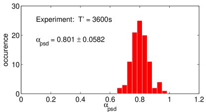
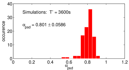
Figure 13: Histograms of experimental (top) and simulated (bottom) fitted values of $\alpha$ for 100 trajectories. Fits are made to the power spectral densities of individual trajectories.

13 (top) we show distribution of $\alpha$ obtained from data analysis of power spectra. The power spectrum method Margolin and Barkai (2005a) yields a single exponent $\alpha_{\textrm{psd}}$ for each stochastic trajectory (which is in our case $\alpha_{+}\approx\alpha_{-}\approx\alpha_{\textrm{psd}}$). Fig. 13 illustrates that the spread of $\alpha$ in the interval $0<\alpha<1$ is not large. Numerical simulation of 100 trajectories switching between 1 and 0, with $\psi_{+}(\tau)=\psi_{-}(\tau)$ and $\alpha=0.8$, and with the same number of bins as the experimental trajectories, was performed and distribution of $\alpha$ values estimated from power spectra is also shown in Fig. 13 (bottom). We observe some spread of measured values of $\alpha$, which is similar to experimental behavior. This indicates that experimental data is compatible with the assumption that all dots are statistically identical (in our sample), in agreement with Brokmann et al. (2003); Issac et al. (2005).

We also tested our nonergodic theory and calculated distribution of relative on times $T^{+}/T$, i.e., of the ratios of the total time in the state on to the total measurement time. These relative on times are equivalent to the experimental time averaged intensities after their “renormalization” in a way making average intensity in state on/off to be 1/0, respectively, in analogy to our model stochastic process. Experimental and simulated distributions shown in Fig.

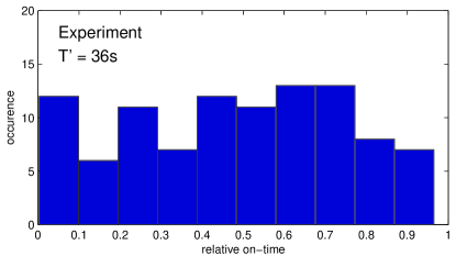
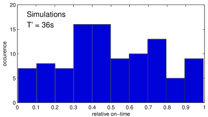
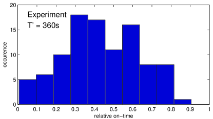
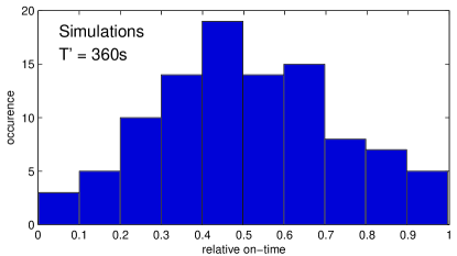
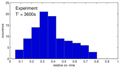
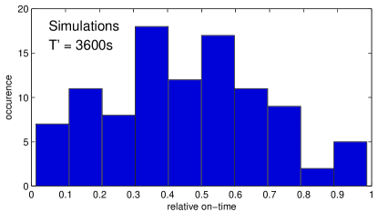
Figure 14: Histograms of relative on times $T^{+}/T$ for 100 experimental (left) and 100 simulated (right) intensity trajectories, for different $T^{\prime}$.

14 are, overall, in good agreement. Two important conclusions are derived from these distributions of relative on times. First the data clearly exhibits ergodicity breaking: distribution of relative on times is not delta peaked, instead it is wide in the interval between 0 and 1, for different $T^{\prime}$. The second important conclusion is that for a reasonably chosen threshold (cf. Fig. 1), the experimental data is compatible with the assumption

$$\psi_{+}(\tau)\approx\psi_{-}(\tau),$$

at least for a wide time window relevant to the experiments. In other words, not only $\alpha_{+}\approx\alpha_{-}$ (ignoring the cutoffs) but also $A_{+}\approx A_{-}$. This observation cannot be obtained directly from the on and off time histograms like Fig. 2 because if only power law tails are seen, as in Fig. 2, these histograms cannot be normalized. To see that $A_{+}\approx A_{-}$ note that the distributions of relative on times are roughly symmetric with respect to the median value of $1/2$ (cf. Fig. 14), and the ensemble average of relative on times is also close to $1/2$, while in general the ensemble average in our model process is given by $A_{+}/(A_{+}+A_{-})$. In addition, the variance of the experimental distributions for different $T^{\prime}$ is close to the variance of the Lamperti distribution $(1-\alpha)/4$ Margolin and Barkai (2005a) for $\alpha\approx 0.8$. There are a few comments to make. First, 100 trajectories are insufficient to produce accurate histograms, as can be seen from the right side of Fig. 14: ideally, these histograms should be identical for different $T^{\prime}$, and given by the Lamperti distribution Eq. (32). Second, there is an effect due to the signal discretization, leading to a flatter and wider histogram at $T^{\prime}=36$s. Third, there is a certain slow narrowing of the experimental histogram as $T^{\prime}$ increases, and the average relative on time slowly decreases. Both of these trends are probably due to cutoffs in the power law distributions, especially for on times, as can be seen in Fig. 2. These trends slightly depend on the choice of the threshold separating on and off states.

As mentioned previously, the groups of Dahan and Bawendi Brokmann et al. (2003); Shimizu et al. (2001) measure values of $\alpha_{+}\approx\alpha_{-}\approx 0.5$ for hundreds of quantum dots (see Table 1), while we report on a higher value of $\alpha$. An important difference between our samples and Dahan/Bawendi groups is that in those works the dots are embedded in PMMA, while in our case they are not [49] (see also Issac et al. (2005)).

VII Summary and Conclusions

Our main points are the following:

1. Simple three-dimensional diffusion model can be used to explain the exponent $\alpha=1/2$ observed in many experiments. In some cases deviations from $\alpha=1/2$ are observed, and modifications of Onsager theory are needed. We cannot exclude other models.

2. Simple model of diffusion may lead to ergodicity breaking. Thus ergodicity breaking in single molecule spectroscopy should not be considered exotic or strange.

3. The time average correlation function is random. Ensemble average correlation function exhibits aging. Hence data analysis should be made with care.

4. Our data analysis shows $A_{+}\approx A_{-}$, $\alpha_{+}\approx\alpha_{-}$ (before the possible cutoffs) and that the distribution of $\alpha$ is narrow. It is important to check the validity of this result in other samples of nanocrystals, since so far the main focus of experimentalist was on values of $\alpha$ and not on the ratio of amplitudes $A_{+}/A_{-}$.

How general are our results? From a stochastic point of view ergodicity breaking, Lévy statistics, anomalous diffusion, aging, and fractional calculus, are all related. In particular ergodicity breaking is found in other models with power law distributions, related to the underlying stochastic model (the Lévy walk). For example the CTRW model also exhibits ergodicity breaking Bel and Barkai (2005), and hence a natural conflict with standard Boltzmann statistics emerges. Since power law distributions are very common in natural behavior, we expect that single particle ergodicity breaking will be a common theme. Further, since we showed that a simple diffusion model can generate ergodicity breaking, for the nano-crystals, we expect that ergodicity breaking be found in other single molecule systems. One simple conclusion is that predictions cannot be made, based on ensemble averages. In fact the time averages of physical observables remain random even in the limit of long measurement time. The fact that the time averaged correlation function is a random function, means that some of the experimental published results, on time average correlation functions, are not reproducible.