Sequence of multipolar transitions: Scenarios for URu₂Si₂

Abstract

$d$- and $f$-shells support a large number of local degrees of freedom: dipoles, quadrupoles, octupoles, hexadecapoles, etc. Usually, the ordering of any multipole component leaves the system sufficiently symmetrical to allow a second symmetry breaking transition. Assuming that a second continuous phase transition occurs, we classify the possibilities. We construct the symmetry group of the first ordered phase, and then re-classify the order parameters in the new symmetry. While this is straightforward for dipole or quadrupole order, it is less familiar for octupole order.

We give a group theoretical analysis, and some illustrative mean field calculations, for the hypothetical case when a second ordering transition modifies the primary ${\cal T}_{xyz}$ octupolar ordering in a tetragonal system like URu₂Si₂. If quadrupoles appear in the second phase transition, they must be accompanied by a time-reversal-odd multipole as an induced order parameter. For ${\cal O}_{xy}$, ${\cal O}_{zx}$, or ${\cal O}_{yz}$ quadrupoles, this would be one of the components of J, which should be easy either to check or to rule out. However, a pre-existing octupolar symmetry can also be broken by a transition to a new octupole–hexadecapole order, or by a combination of ${\cal O}_{2}^{2}$ quadrupole and triakontadipole order.

It is interesting to notice that if recent NQR results[1] on URu₂Si₂ are interpreted as a hint that the onset of octupolar hidden order at $T_{0}=17{\rm K}$ is followed by quadrupolar ordering at $T^{*}\approx 13.5{\rm K}$, this sequence of events may fit several of the scenarios found in our general classification scheme. However, we have to await further evidence showing that the NQR anomalies at $T^{*}\approx 13.5{\rm K}$ are associated with an equilibrium phase transition.

1 Introduction

There is increasing interest in orbital ordering phenomena, and their relationship to magnetism[3, 4, 5]. Many of these phenomena can be at least partially understood in terms of localized electron models. This is clearly justified for Mott-localized $d$-electrons. Some $f$-electron systems are semiconductors (like NpO₂), but more often, we wish to describe multipole ordering in metals like rare-earth-filled skutterudites or URu₂Si₂. In the standard model[6] of the majority of rare earth elements the $f$-shell is localized, and we may invoke a similar feature for the systems of interest to us. It can be argued that itineracy and multipolar ordering are complementary features, and that they may be manifest in different phases of the same $f$-electron system. In this case, the localized description is acceptable for the ordered phases, even though we know that it could not be extended to the whole phase diagram.

The common starting point is the existence of an $N$-dimensional local Hilbert space $|n\rangle$, which allows the definition of $N^{2}$ local operators $|n\rangle\langle m|$ (of these, $N^{2}-1$ are non-trivial, and are also called local order parameters). $N(N+1)/2$ operators have symmetrical, and $N(N-1)/2$ operators have antisymmetrical character. They can be chosen as

$$X_{mn}^{s}=\frac{1}{2}(|m\rangle\langle n|+|n\rangle\langle m|)$$ (1)

for symmetrical and

$$X_{mn}^{a}=\frac{1}{2i}(|m\rangle\langle n|-|n\rangle\langle m|)$$ (2)

for antisymmetrical operators where $i$ was inserted to ensure hermiticity.

There are two canonical cases: the basis may consist of

1. N/2 time-reversed pairs (the N-fold degeneracy arises as 2${\times}$(N/2),
   (Kramers degeneracy)${\times}$(non-Kramers degeneracy)

2. real basis states each of which is time reversal invariant (the N-fold degeneracy is purely non-Kramers degeneracy)

Case I. The local Hilbert space consists of $(N/2)$ time-reversed pairs. There are $N(N-1)/2$ time-reversal-even order parameters (this includes the trivial ${\hat{1}}$), and $N(N+1)/2$ time-reversal-odd order parameters.

$N=4$ is realized by the $\Gamma_{8}$ representation of the cubic double group, the irrep of the ground state level for either the $4f^{1}$ compound CeB₆ (Refs. [7, 8]), or the $5f^{3}$ compound NpO₂ (Ref. [9]). Six operators: ${\hat{1}}$ and the five quadrupoles are time-reversal-even, while ten order parameters: the three dipoles and seven magnetic octupoles, change sign under time reversal. A general form of intersite interaction is a sum over the quadratic invariants, for a cubic system with six independent coupling constants (one dipolar, two quadrupolar, three octupolar). It was, however, soon realized[7] that the consideration of the SU(4) symmetrical model (with all couplings set equal) should be enlightening. Later research showed that CeB₆ can be regarded as a ”nearly SU(4)-symmetrical” system[10, 11].

Case II. If all basis states can be chosen real, the $X_{m,n}^{s}$ are real operators and the $X_{m,n}^{a}$ are imaginary operators. Choosing one of the real operators as the projection onto the entire local Hilbert space ${\hat{\boldmath 1}}=\sum_{m}|m\rangle\langle m|$, and orthogonalizing the remaining $N-1$ diagonal operators, we are left with $N(N+1)/2-1$ time-reversal invariant local order parameters. $N(N-1)/2$ local order parameters (the imaginary operators $X_{m,n}^{a}$) change sign under time reversal.

This case is realized for non-Kramers ions which have an even number of electrons. We are interested in the $5f^{2}$ (U⁴⁺), and $4f^{2}$ (Pr³⁺) configurations as they appear in URu₂Si₂ and PrFe₄P₁₂, resp. It is always debatable which $N$ to choose. Crystal field doublets ($N=2$) have been suggested for both systems but it is unlikely for PrFe₄P₁₂, and at least not widely accepted for URu₂Si₂. In fact, for both systems we settle for a local Hilbert space which is composed of the bases of several irreps. For PrFe₄P₁₂ the quasi-quartet[12] $\Gamma_{1}+\Gamma_{4}$ seems to work. Under tetrahedral symmetry, the nine time-reversal-even order parameters are a singlet, five quadrupoles, and three hexadecapoles, while the six time-reversal-odd order parameters are three dipoles and three octupoles[13].

1.1 The nature of the higher multipoles

While dipoles and quadrupoles are well-known from decades of research experience, it is only recently that octupoles were seriously considered, and higher multipoles are virtually never discussed. It is worth forming a picturial idea of octopule-, hexadecapole-, and triakontadipole-carrying shells.

The $J=4$ Hund’s rule two-electron states of U${}^{4+}=5f^{2}$ ionic cores are rather complicated objects, superposed of a number of $l_{j}s_{j}$ components by the Clebsch-Gordan coefficients. However, there is strong similarity between the multipoles composed of two $f$-orbitals and two spins via a number of projections, and simplified multipoles built of $l=4$ orbitals (atomic $g$-states). We derive the charge cloud shapes and current distribution patterns from acting with the analogous purely orbital (e.g., ${\overline{J_{z}(J_{x}^{2}-J_{y}^{2})}}\rightarrow{\overline{l_{z}(l_{x}^{2}-l_{y}^{2})}}$) operators on fictitious atomic states (for our purposes, fourth-order spherical harmonics $Y^{4}_{m}(\vartheta,\phi)$ for $g$-states). In this Section, we do not discuss crystal field effects.

We diagonalize multipole operators in the 9-dimensional $l=4$ space, and base our pictures on the state with the (in absolute value) largest eigenvalue. This can be interpreted as finding the ground state of an effective field which orders the multipole. We mention that free-ion multipole eigenstates are not necessarily the same that we find within the restricted Hilbert spaces of crystal field problems. This will be illustrated by comparing Fig. 2 and Fig. 5. Furthermore, smaller Hilbert spaces may not give a representation of certain multipoles at all.

For odd-rank (magnetic) multipoles, the eigenstates appear in time-reversed pairs, similar to the $l_{z}=\pm m$ dipole eigenstates, and the multipole spectrum is symmetrical about 0. For even-rank (electric) multipoles, each eigenstate can be chosen time-reversal invariant.

1.1.1 Octupoles

First, let us consider the octupole

$${\cal T}_{xyz}\rightarrow\frac{1}{6}{\overline{l_{x}l_{y}l_{z}}}=\frac{-i}{4}\left(l_{+}l_{z}l_{-}-l_{-}l_{z}l_{-}\right)$$ (3)

The simplest octupolar states are realized in the $l=2$ subspace of $e_{g}$ functions

$$\Phi_{\pm}(l=2)=\frac{1}{\sqrt{2}}\left(|3z^{2}-r^{2}\rangle\pm i|x^{2}-y^{2}\rangle\right)$$ (4)

$\Phi_{\pm}(l=2)$ form a time-reversed pair.

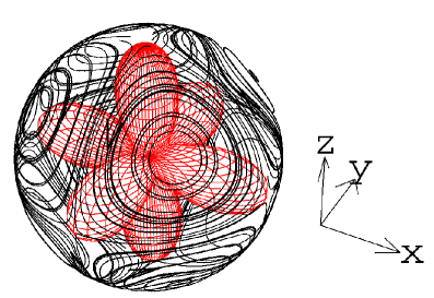
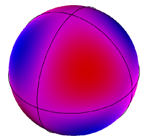
Figure 1: Left: Charge distribution (lobes) and current pattern (flow lines) in the ${\cal T}_{xyz}$ octupole eigenstate $\Phi_{+}$ in the $l=2$ Hilbert space. Right: the normal component of the magnetic field is pointing inwards (outwards) in the light grey (dark grey) areas.

The charge and the current distribution of $\Phi_{+}(l=2)$ is shown in Fig. 1. The object got its name from the eight magnetic poles: of the eight current eddies we see in the figure, four belong to magnetic field lines entering, and four to those leaving the surface. Note that the magnetic field pattern measured[14] by $\mu$SR in NpO₂ bears an overall similarity to what we expect in the neighborhood of an octupole-moment bearing shell. For the time-reversed partner $\Phi_{-}(l=2)$ we would find the same charge cloud with reversed currents.

The concept of octupolar ordering was pioneered by Korovin and Kudinov[15] who envisaged an antiferro-octupole pattern of the $e_{g}$ states (4) resulting from spin-orbital exchange in Mott insulators. A similar possibility arises in the $E$ doublets of trigonal compounds[16] where, however, the octupole moment is mixed with the orbital moment $l_{z}$. In any case, antiferro-orbital order is likely to be combined with spin ferromagnetism[17, 18, 19]. Metallic phases, including the itinerant octupolar phase, were investigated for the $e_{g}$ band Hubbard model by Takahashi and Shiba[17].

Currently known realizations of octupolar order appear in $f$-electron systems. Field-induced octupoles play a role in understanding the phase diagram of CeB₆ (Ref. [8]). Kusunose and Kuramoto[20] called attention to the fact that octupole moments are ideally suited for the role of ”hidden” primary order parameters. A detailed study by Kubo and Kuramoto[21] makes a convincing case that the ”Phase IV” of Ce_1-xLa_xB₆ is an antiferro-octupolar phase. At about the same, it became accepted that the long-standing mystery of the nature of the 25K transition of NpO₂ is solved by identifying it with the triple-q ordering of $\Gamma_{5u}$ octupoles[22, 23, 24]. A symmetry analysis was successful in identifying the unique octupolar signature in NMR spectra on NpO₂, and Ce_1-xLa_xB₆ (Ref. [25]. The phenomenology of the two systems shows certain similarities, as it is to be expected since, e.g., the relationship between the anomalies of the linear, and the third-order, susceptibilities follow from general thermodynamic reasoning[23, 26]. The same should be true of URu₂Si₂ whos hidden order, we argued[2], is also of octupolar nature.

Fig. 1 illustrates the symmetry of the (uniform) octupolar ground state with $\langle{\cal T}_{xyz}\rangle$ as the order parameter. We leave to Sec. 3.2 the construction of an octupolar symmetry group, which will be carried out for a combination of tetragonal crystal field and octupolar effective field, the case relevant for URu₂Si₂. Here we use Fig. 1 to visualize the hybrid nature of some of the symmetry elements. The charge distribution is highly symmetrical (octahedral). However, the true symmetry is that of the magnetic field pattern, so in purely geometrical terms it is tetrahedral. It is obvious, however, that ${\cal C}_{4}$ rotations are allowed if they are combined with time reversal ${\cal T}$ (which reverses the currents and the field). Including elements like ${\cal C}_{4}{\cal T}$, a higher non-unitary symmetry group could be derived.

Figure. 1 shows why octupolar order can be so well ”hidden”. The charge distribution (which influences directional bonding, i.e., the structure of the crystal) is cubic, hiding the fact that if current directions are considered, the pure ${\cal C}_{4}$ axes are not symmetry elements. Similar considerations arose when it was asked whether the pseudocubic phase of Sr-doped LaMnO₃ is not, in fact, octupolar ordered[17].

One might have thought that the character of the octupoles is the same whatever Hilbert space we represent them on, but there are interesting nuances here.

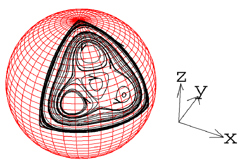
Figure 2: Current distribution in the ${\cal T}_{xyz}$ octupole ground state (5) in the $l=4$ Hilbert space. Only one octant is shown.

Within the $l=4$ shell (which mimicks URu₂Si₂’s $5f^{2}\rightarrow J=4$ multiplet), ${\cal T}_{xyz}$ has the minimal eigenvalue $-6\sqrt{3}$, corresponding to the eigenstate (expressed in the $|l_{z}\rangle$ basis)

$$\Phi^{\rm oct}_{0}=\sqrt{\frac{7}{50}}(|+4\rangle+|-4\rangle)-2i\sqrt{\frac{3}{50}}(|+2\rangle+|-2\rangle)-\sqrt{\frac{1}{5}}|0\rangle$$ (5)

(the maximal eigenvalue $6\sqrt{3}$ corresponds to the time-reversed of $\Phi^{\rm oct}_{0}$). The current distribution for $\Phi^{\rm oct}_{0}$ is shown in Fig. 2. The overall pattern of eight alternating vortices is the same as in Fig. 1. However, within each of the major eddies four new sub-eddies appear: three (arranged like the petals of a flower) rotating in the sense of the eddy as a whole, and a little central eddy counter-rotating. The symmetry of the current distribution in Fig. 2 is the same as that in Fig. 1, but there are differences in the magnetic field pattern. While in Fig. 1 the magnetic field is maximum in the center of an octant, and has the same sign everywhere within the octant, in the $l=4$ solution (Fig. 2) the field changes sign in a small central region of the octant and appears smaller than in the ”petals”. On the whole, the magnetic field of the octupolar currents is weaker for $l=4$ states ($f^{2}$ configurations) than for the simplest $l=2$ solution. This may account for the weakness of the internal fields in URu₂Si₂. It should be noted, though, that the current distribution shown in Fig. 2 was obtained for a free ion subject to the octupolar effective field only. The situation changes if crystal field effects are included (Sec. 3.2).

It would be of obvious interest to calculate internal field distributions for octupoles, and maybe also for triakontadipoles, for these predictions could be checked against $\mu$SR and NMR observations. We note that Kubo and Kuramoto[21] discussed the situation for the two well-established octupolar systems NpO₂ and Ce_1-xLa_xB₆. for which 500G and 40G, respectively, are measured; both are in excess of the theoretical estimate. The measured internal field in URu₂Si₂ is much weaker: ²⁹Si-NMR linewidth gives $\leq 12$G (Ref.[27]), while at the muon stopping sites, the internal field is at most 1–2G (Ref.[28]).

1.1.2 Hexadecapoles

The hexadecapole ${\overline{l_{x}l_{y}(l_{x}^{2}-l_{y}^{2})}}$ has the largest eigenvalue for the eigenstate

$$\Phi_{\rm hex}=\frac{1}{\sqrt{2}}(|2\rangle-i|-2\rangle)\,.$$ (6)

In spite of the appearance of $i$, $\Phi_{\rm hex}$ is time reversal invariant. It can be chosen real and its positive and negative lobes can be identified (Fig. 3). There is a general similarity to quadrupolar eigenstates (which also have positive and negative lobes), only the number of lobes is higher. We do not construct the symmetry group of the hexadecapole effective field but we notice that, like the octupolar symmetry group, it would have composite symmetry elements: purely geometrical transformations combined with ”lobe sign reversal”.

Hexadecapoles as order parameters were discussed within the tetrahedral symmetry classification[13], valid for Pr-filled skutterudites. We are not aware of the existence of primary hexadecapole order in any system.

1.1.3 Triakontadipoles

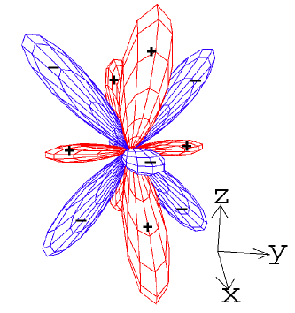
Figure 3: Charge distribution in the electric hexadecapole eigenstate (6). The sign of the lobes of the wave function is also shown.

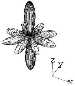
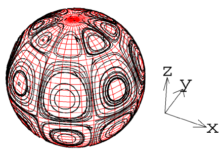
Figure 4: The charge (left) and the current (right) distribution in the magnetic triakontadipole eigenstate (7).

There are 11 triakontadipoles but we consider only ${\overline{l_{x}l_{y}l_{z}(l_{x}^{2}-l_{y}^{2})}}$ which appears as the lowest-rank $A_{1u}$ multipole in the tetragonal classification (Table 1). Its ground state is

$$\Phi_{\rm tria}=\frac{1}{2}\left(|4\rangle+|-4\rangle+i\sqrt{2}|0\rangle\right)\,.$$ (7)

with eigenvalue $6\sqrt{35}$. As shown in Fig. 4, there are 32 cells of alternatingly flowing current, so the associated magnetic field is more short-ranged than in the case of an octupole (Fig. 1). As in the case of octupoles, the symmetry of the charge distribution is higher than that of the current distribution: the charge cloud has a ${\cal C}_{8}$ axis which is reduced to ${\cal C}_{4}$ for the currents. However, the combination of the $\pi/4$ rotation with time reversal ${\cal C}_{8}{\cal T}$ is a symmetry operation. It would be interesting to meet triakontadipolar order in nature.

2 Recent experimental developments on URu₂Si₂

The magnetic behavior and phase diagram of the intermetallic compound URu₂Si₂ have been the focus of attention for over two decades[29]. Specific heat measurements [30] show that electronic entropy of $O(\ln{2}){\cdot}k_{\rm B}$ is released by the time the temperature reaches 30K, and a sizeable fraction of it is associated with the $\lambda$-anomaly at $T_{0}\approx 17{\rm K}$. Thus it is not unjustified to think of the phase transition as the full-scale ordering of a localized degree of freedom, but the nature of the order parameter remains hidden. It is obviously not the tiny ($\sim 0.03{\mu}_{\rm B}$) antiferromagnetic moment which is observed by neutron scattering [31].

Small (either static or slowly fluctuating) moments have long been held to be an attribute of heavy fermion systems on the borderline between localized and itinerant $f$-electron phases. The specific heat value would allow to classify URu₂Si₂ as a ”light heavy fermion system”, raising the question whether its mysterious properties may be related to an exotic itinerant phase of strongly correlated $f$-electrons. Orbital magnetism due to plaquette currents[32], unconventional density waves[33, 34], and Pomeranchuk instability leading to a nematic state[35] are in this category.

The RKKY interaction mediates a variety of multipole-multipole interactions between the $f$-shells[36]. However, the ordering may be foiled by the collective Kondo effect: the formation of a heavy Fermi sea with a large (Luttinger) Fermi surface[37] may swallow up the localized moments. The Kondo-to-RKKY transition has been extensively studied for the case when the relevant local degrees of freedom are spin dipoles[38] but work on the general multipolar problem has only just started[39]. It is an intriguing possibility that the 17K phase transition in URu₂Si₂ coincides with the itinerant-to-localized transition of the $f$-electrons[40]. This would lend credence to describing the $T<T_{0}$ order in terms of a localized $f$-electron model even if a more satisfactory description will have to encompass itinerant aspects[41].

It has long been known[43, 42] that the symmetry classification of local order parameters in tetragonal crystal fields follows Table 1. For each of the irreps, only the lowest-rank multipole is listed. The result can be viewed as arising from the tetragonal splitting of the operator irreps of the cubic classification scheme[8].

Table 1: Symmetry classification of the local order parameters for ${\bf B}=0$ (${\cal D}_{4h}$ notations [44], overline means symmetrization). $g$ ($u$) belongs to even (odd) parity under time reversal.

sym ($g$)	operator	sym ($u$)	operator
$A_{1g}$	${\cal E}$	$A_{1u}$	${\overline{J_{x}J_{y}J_{z}(J_{x}^{2}-J_{y}^{2})}}$
$A_{2g}$	${\cal H}_{1}={\overline{J_{x}J_{y}(J_{x}^{2}-J_{y}^{2})}}$	$A_{2u}$	$J_{z}$
$B_{1g}$	${\cal O}_{2}^{2}$	$B_{1u}$	${\cal T}_{xyz}={\overline{J_{x}J_{y}J_{z}}}$
$B_{2g}$	${\cal O}_{xy}={\overline{J_{x}J_{y}}}$	$B_{2u}$	${\cal T}^{\beta}_{z}={\overline{J_{z}(J_{x}^{2}-J_{y}^{2})}}$
$E_{g}$	$\{{\cal O}_{xz},{\cal O}_{yz}\}$	$E_{u}$	$\{J_{x},J_{y}\}$

Progress with uncovering the true nature of the hidden order of URu₂Si₂ has been particularly slow because of a seemingly extrinsic property of almost all of the samples: they show a kind of micro-antiferromagnetism with moments $m\sim 0.02-0.04{\mu_{\rm B}}\parallel{\hat{z}}$ with the simple alternating order ${\bf Q}=(0,0,1)$[43]. However, evidence from microscopic measurements[45, 46, 47, 28] shows that the nominally small moment should be understood as a relatively large moment at a minority of the sites.

The relationship between the hidden order parameter $\psi$ and the antiferromagnetic moment $m$ has been, and still remains[50], a matter of debate. There are two basic possibilities[48]: A) hidden order and antiferromagnetism share the same symmetry[49], or B) they are of different symmetries. In Case A), the relative amplitude of $m$ and $\psi$ can be tuned continuously (e.g., by pressure), and there is no sharp distinction between the two orders. In Case B), the two orders are incompatible, and there must be a first order transition from the $\psi\neq 0$, $m=0$ phase to the $\psi=0$, $m\neq 0$ phase. In the present discussion (as in Ref.[2]) we take the conclusion drawn from recent $\mu$SR experiments[28] as our starting point: there is a first-order transition, the symmetry of $\psi$ is different from that of $m$, and therefore the hidden order parameter must be sought from among other entries in Table 1.

As far as gross features like linear and non-linear[51] susceptibility, specific heat, etc. are concerned, with a little adjustment of the crystal field level scheme, $B_{1g}$ and $B_{2g}$ quadrupolar [52], and $B_{1u}$ and $B_{2u}$ octupolar [2] models do about equally well. Evidence beyond this simple range of experiments has to be invoked to choose between the quadrupolar and octupolar scenarios.

We cite two crucial (but as yet unpublished) experiments to argue that the hidden order is not quadrupolar. First, there is a remarkable mechanical–magnetic cross–effect (at $T<17$K): in the presence of uniaxial stress applied perpendicularly to the tetragonal main axis, large-moment antiferromagnetism with the simple pattern described above becomes visible for neutron magnetic Bragg scattering [53]. This is unambiguous proof that the background order breaks time reversal invariance, and is thus certainly not quadrupolar; the simplest remaining choice is octupolar order.

The second evidence is coming from recent NQR measurements by Saitoh et al [1]. The temperature dependence of the electric field gradients was followed carefully from relatively high temperatures (70K) to well below $T_{0}=17$K. $V_{zz}$ changes all the time, reflecting the $T$-dependence of the tetragonal crystal field component ${\cal O}_{2}^{0}$. Saitoh et al’s findings can be formulated in two statements: (a) Neither of the field gradients shows anomalies at $T_{0}=17$K, the onset temperature of hidden order, so the hidden order cannot be quadrupolar. (b) There is an anomaly in the NQR signal at $T^{*}\approx 13.5$K, so something happens to the quadrupoles there. A possibility is that $T^{*}$ is the ordering transition of quadrupoles; then it has to be a second HO transition following the first one at $T_{0}$. We emphasize that a lot more experimental evidence (especially specific heat, susceptibility, etc) is needed before the existence of a phase transition at $T^{*}$ may become accepted. It is not our aim to describe the two transitions in any detail. We merely emphasize that, given the symmetry of URu₂Si₂, octupolar ordering can be followed by quadrupolar ordering; but then further induced magnetic multipoles should be observable.

While circumstantial evidence for octupolar ordering looks encouraging, attempts for its direct verification have as yet yielded negative results. An early, very specific neutron scattering investigation ruled out either $B_{1u}$ or $B_{2u}$ octupoles at the selected wavevectors, including the (0,0,1) periodicity of the weak-moment antiferromagnetism[43]. It has been argued that resonant X-ray scattering would not see the octupoles[54]. Last, but not least, though the octupolar scenario is as yet the only one to account for the observed fact that transverse uniaxial stress induces $\parallel{\hat{z}}$ antiferromagnetism, in a simple mean field version[2] it forces a choice between $\sigma\parallel(100)$ and $\sigma\parallel(110)$ directions of stress, while experiments seem to tell us that these directions are equivalent[53]. An essential insight is missing here.

A microscopic theory will have to address the questions raised above. Our present investigation is of a limited scope: we use general arguments to classify the symmetry-allowed ordering transitions of URu₂Si₂. We are particularly interested in the possibility of a sequence of such continuous phase transitions. We have no statement to make if the lower-temperature transition is of first order.

We address the simplest questions for which no knowledge of microscopic details is required: Once we had an octupolar ordering transition, is there any compelling reason to expect a second symmetry-breaking transition? What may be the order parameters? Should we expect still more, as yet undiscovered, phase transitions?

In an abstract sense, our question is the following: assuming the symmetry of the high-temperature (”para”) symmetry group ${\cal G}_{\rm para}$ has been broken by a spontaneous ordering transition, introducing order $\langle{\cal O}_{1}\rangle\neq 0$ lowers the symmetry to ${\cal G}({\cal O}_{1})\in{\cal G}_{\rm para}$. What is the structure of ${\cal G}({\cal O}_{1})$? What is the new classification of the order parameters? Assuming that such order parameters are found, does this imply that further continuous phase transitions necessarily happen?

In Ref.[2], we discussed in some detail two questions of this nature: the symmetry classification of the order parameters in the presence of an 1) external magnetic field ${\cal B}\parallel{\hat{z}}$, and 2) a uniaxial stress. Formally the same question arises if instead of externally applied fields, we assume the presence of an effective field associated with either a dipole ordering transition (1) or quadrupolar order (2).

In Sec. 3.1, we rephrase our earlier results on the effect of an external magnetic field, and add some remarks about the field direction dependence. In Sec. 3.2, we analyze the symmetry in the presence of a ${\cal T}_{xyz}$ octupolar (effective) field, and the possibility of a sequence of phase transitions. Sec. 4 illustrates the general arguments with a simple mean field calculation.

3 Symmetry lowering in external, or effective, fields

3.1 Magnetic field

In the presence of an external magnetic field $H_{z}\parallel(0,0,1)$ or equivalently $\langle J_{z}\rangle>0$, the remaining purely geometrical symmetry elements are ${\cal E}$, $2{\cal C}_{4}$, and ${\cal C}_{2}^{2}$ (and, naturally, the inversion ${\cal I}$). The geometrical symmetry (described by unitary operations) is lowered to ${\cal C}_{4h}$, but the full symmetry group ${\cal G}_{\rm tetr}(J_{z})$ contains also non-unitary elements, namely $2{\cal C}_{2}^{\prime}{\cal T}$, and $2{\cal C}_{2}^{\prime\prime}{\cal T}$, where ${\cal T}$ is time reversal. ${\cal G}_{\rm tetr}(J_{z})$ contains eight elements, its character table (and multiplication table) is the same as that of the tetragonal point group ${\cal D}_{4}$. The character table is given in Table 2.

Reducing the symmetry from ${\cal G}_{\rm tetr}$ to ${\cal G}_{\rm tetr}(J_{z})$, some of the originally inequivalent irreps of ${\cal G}_{\rm tetr}$ become equivalent. This parentage of the irreps is shown in Table 2. It also follows that the corresponding order parameters get mixed. This was discussed in Ref. [2].

Table 2: Character table of the non-unitary symmetry group ${\cal G}_{\rm tetr}(J_{z})$ of a tetragonal system placed in a magnetic field ${\bf B}=(0,0,B_{z})$. Space inversion is omitted.

${\rm irrep}$	${\cal E}$	$2{\cal C}_{4}$	${\cal C}_{4}^{2}$	$2{\cal C}_{2}^{\prime}{\cal T}$	$2{\cal C}_{2}^{\prime\prime}{\cal T}$	parentage	operators
$A_{1}$	1	1	1	1	1	$A_{1g}$, $A_{2u}$	1, $J_{z}$
$A_{2}$	1	1	1	-1	-1	$A_{1u}$, $A_{2g}$	${\overline{J_{x}J_{y}(J_{x}^{2}-J_{y}^{2})}}$, ${\overline{J_{x}J_{y}J_{z}(J_{x}^{2}-J_{y}^{2})}}$
$B_{1}$	1	-1	1	1	-1	$B_{1g}$, $B_{2u}$	${\cal O}_{2}^{2}$, ${\cal T}^{\beta}_{z}={\overline{J_{z}(J_{x}^{2}-J_{y}^{2})}}$
$B_{2}$	1	-1	1	-1	1	$B_{2g}$, $B_{1u}$	${\cal O}_{xy}$, ${\cal T}_{xyz}$
$E$	2	0	-2	0	0	$E_{g}$, $E_{u}$	{ $J_{x}$, $J_{y}$ } , { ${\cal O}_{xz}$, ${\cal O}_{yz}$ }

${\hat{x}}$ is a lower-symmetry direction than ${\hat{z}}$ and correspondingly a system subjected to a magnetic field ${\bf B}=(B_{x},0,0)$ has a smaller symmetry group ${\cal G}_{\rm tetr}(J_{x})$ (Table 3). In contrast to the case ${\bf B}\parallel{\hat{z}}$ where irreps taken from the zero field case kept their dimensionality only pairwise merged, now the two-dimensional irreps split. The parentage of the ${\bf B}\parallel{\hat{x}}$ irreps is as follows $A_{1g},B_{1g}\longrightarrow\Gamma_{1}$, $A_{2g},B_{2g}\longrightarrow\Gamma_{2}$, $A_{1u},B_{1u}\longrightarrow\Gamma_{3}$, $A_{2u},B_{2u}\longrightarrow\Gamma_{4}$, $E_{g}\longrightarrow\Gamma_{3}+\Gamma_{4}$, $E_{u}\longrightarrow\Gamma_{1}+\Gamma_{2}$.

Table 3: Character table of the non-unitary symmetry group ${\cal G}_{\rm tetr}(J_{x})$

${\rm irrep}$	${\cal E}$	${\cal C}_{4}^{2}{\cal T}$	${\cal C}_{2x}^{\prime}$	${\cal C}_{2y}^{\prime}{\cal T}$
$\Gamma_{1}$	1	1	1	1
$\Gamma_{2}$	1	1	-1	-1
$\Gamma_{3}$	1	-1	1	-1
$\Gamma_{4}$	1	-1	-1	1

The presence of non-identity irreps in Tables 2 and 3 shows that for fields ${\bf B}\parallel{\hat{z}}$, and even for ${\bf B}\parallel{\hat{x}}$, a variety of symmetry breaking transitions are possible. Since the field has broken time reversal invariance, and induced a polarization in its direction, all these transitions have the character of orbital ordering (lifting some residual non-Kramers degeneracy), and also lead to the appearance of time-reversal-odd transverse polarization components. We enumerate the possibilities (${\bf B}\parallel{\hat{z}}$)

• A field ${\bf B}\parallel{\hat{z}}$ allows the ordering of $E$ type quadrupoles and this is accompanied by the appearance of dipole polarization in the $xy$ plane. This was suggested[2] for the disjoint high-field phase observed in experiments[55] on URu₂Si₂. Analogous phenomena are observed[56] in high field experiments on the tetrahedral skutterudite PrOs₄Sb₁₂.

• The ordering is of $B_{1}$ type. In our suggestion[2] for the low-field order of URu₂Si₂, the primary order was ${\cal T}_{z}^{\beta}$ octupolar (this survives when the field is switched off), and ${\cal O}_{2}^{2}$ quadrupoles were field-induced. Santini’s scenario[52] was the opposite: primary quadrupolar order, and field-induced octupoles.

• $B_{2}$ order parameters: primary ${\cal T}_{xyz}$ octupolar order and field-induced ${\cal O}_{xy}$ quadrupoles. In the present paper, we assume this is the hidden order with onset temperature $T_{0}=17$K. Lacking a microscopic model, it is impossible to decide between this scenario and the previous $B_{1}$ scheme.

• The exotic possibility of $A_{2}$ order: ${\cal H}_{1}$ hexadecapoles and ${\overline{J_{x}J_{y}J_{z}(J_{x}^{2}-J_{y}^{2})}}$ triakontadipoles, has not been considered yet.

The discussion of the cases ${\bf B}\parallel{\hat{y}}$ and ${\bf B}\parallel({\hat{x}}\pm{\hat{y}})$ would be analogous to ${\bf B}\parallel{\hat{x}}$: the remaining symmetry group has order 4 (or 8, if we include inversion). The symmetry group for fields lying in the $x$–$y$ plane in non-special directions is generated by ${\cal C}_{4}^{2}{\cal T}$ and ${\cal I}$. For fields in general out-of-plane directions, the only remaining symmetry is inversion.

We conclude that a spontaneous symmetry breaking transition in external fields remains possible if the field is either parallel or perpendicular to ${\hat{z}}$. In particular, the octupolar transition can remain second order for a range of field strengths. However, ${\cal T}_{xyz}$ octupoles get mixed with ${\cal O}_{xy}$ ($B_{2}$) quadrupoles for ${\bf B}\parallel{\hat{z}}$, and with $E$-derived quadrupoles (a suitable combination of ${\cal O}_{yz}$ and ${\cal O}_{xz}$) for ${\bf B}\perp{\hat{z}}$. For general field directions, a smearing of the octupolar transition should be observed. This effect may be helpful in deciding whether the hidden order is of octupolar nature.

The above reasoning can also be extended to discuss further symmetry breakings after a phase transition to a dipole-ordered phase has taken place. The effective field of the ordered moments acts the same way as an external field. E.g., we may conclude that following a transition to a $\langle J_{z}\rangle\neq 0$ phase at the higher critical temperature $T_{c}^{>}$, tranverse dipoles (from the $E$ doublet $\{J_{x},J_{y}\}$) may also order at a lower critical temperature $T_{c}^{<}$, and that $\langle J_{x}\rangle\neq 0$ induces $\langle{\cal O}_{xz}\rangle\neq 0$. Though symmetry allows this (or some other scenario identifiable from Table 2) to happen, whether this potentiality is realized depends on the nature of the microscopic model.

3.2 The symmetry group of the octupolar phase

We may ask whether following the onset of, say, ${\cal T}_{xyz}$ type octupolar order a further symmetry lowering transition is possible. This is the same question as to whether spontaneous symmetry breaking in an external octupolar field of $B_{1u}$ symmetry is possible. The question is partly academical, but it is also motivated by the NQR findings on URu₂Si₂ by Saitoh et al[1]. In particular, they claimed that either ${\cal O}_{xy}$ or ${\cal O}_{2}^{2}$ quadrupoles appear at $T^{*}\approx 13.5{\rm K}$, well below $T_{0}\approx 17{\rm K}$ which we associate with the onset of octupolar order. However, as we emphasized before, the connection of our arguments with experiments remains tenuous.

We have to identify which operations leave the ${\cal T}_{xyz}$ octupoles unchanged, i.e., we are looking for the octupolar symmetry group ${\cal G}_{\rm tetr}({\cal T}_{xyz})$ as a subgroup of ${\cal G}_{\rm tetr}$. Schematically, ${\cal T}_{xyz}$ is represented in Fig. 5 where the current distribution in the ground state of ${\cal T}_{xyz}$ is shown for two- and three-dimensional subspaces selected from the 9-dimensional Hilbert space of the tetragonal crystal field eigenstates[2, 52]. It is obvious that the selection of the basis functions (which is ”done” by the crystal field potential) has a strong influence on the details of the current pattern. However, though the pattern is much more decorated for the $\{|t_{1}\rangle,|t_{3}\rangle\}$ doublet than for the triplet $\{|t_{1}\rangle,|t_{2}\rangle,|t_{4}\rangle\}$ (the crystal field model used in Ref.[2]), the symmetries are the same. In either case, there is a current distribution with eight major eddies: four positive, and four negative (whether within these, there are sub-eddies, has no influence on the symmetry). Though there are local magnetic fields, the total magnetic moment is zero. A ${\cal C}_{4}$ rotation takes positive eddies into negative ones, and vice versa; however, reversing also the direction of currents, the original state is restored. From the ${\cal C}_{2}^{\prime}$ and ${\cal C}_{2}^{\prime\prime}$ elements of ${\cal G}_{\rm tetr}$, the latter two have to be combined with ${\cal T}$. The character table of the symmetry group ${\cal G}_{\rm tetr}({\cal T}_{xyz})$ is shown in Table 4 (as before, it is understood that the space inversion ${\cal I}$ would generate the other half of the complete symmetry group). We have also given the resulting symmetry classification of some of the order parameters in the last column of Table 4.

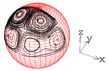
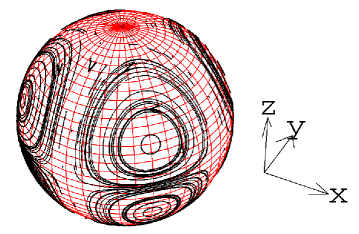
Figure 5: Crystal field effects on the current distribution in the ${\cal T}_{xyz}$ octupole ground state. Left: the doublet $\{|t_{1}\rangle,|t_{3}\rangle\}$ ($|t_{3}\rangle=(1/\sqrt{2})(|2\rangle+|-2\rangle)$). Right: the triplet $\{|t_{1}\rangle,|t_{2}\rangle,|t_{4}\rangle\}$ (10)–(12). The two current distributions have the same symmetry given in Table 4.

Table 4: Character table of the non-unitary symmetry group ${\cal G}_{\rm tetr}({\cal T}_{xyz})$ of a tetragonal system placed in an effective octupolar field. Space inversion is omitted.

${\rm irrep}$	${\cal E}$	$2{\cal C}_{4}{\cal T}$	${\cal C}_{4}^{2}$	$2{\cal C}_{2}^{\prime}$	$2{\cal C}_{2}^{\prime\prime}{\cal T}$	parentage	operators
$A_{1}$	1	1	1	1	1	$A_{1g}$, $B_{1u}$	1, ${\cal T}_{xyz}$
$A_{2}$	1	1	1	-1	-1	$A_{2g}$, $B_{2u}$	${\overline{J_{x}J_{y}(J_{x}^{2}-J_{y}^{2})}}$, ${\cal T}^{\beta}_{z}={\overline{J_{z}(J_{x}^{2}-J_{y}^{2})}}$
$B_{1}$	1	-1	1	1	-1	$B_{1g}$, $A_{1u}$	${\cal O}_{2}^{2}$, ${\overline{J_{x}J_{y}J_{z}(J_{x}^{2}-J_{y}^{2})}}$
$B_{2}$	1	-1	1	-1	1	$B_{2g}$, $A_{2u}$	${\cal O}_{xy}$, $J_{z}$
$E$	2	0	-2	0	0	$E_{g}$, $E_{u}$	{ $J_{x}$, $J_{y}$ } , { ${\cal O}_{xz}$, ${\cal O}_{yz}$ }

It is interesting to note the similarities and dissimilarities to the symmetry group of $J_{z}$ (Table 2). The character table is the same only in ${\cal G}_{\rm tetr}({\cal T}_{xyz})$, $2{\cal C}_{4}$ and $2{\cal C}_{2}^{\prime}$, while in ${\cal G}_{\rm tetr}(J_{z})$, $2{\cal C}_{2}^{\prime}$ and $2{\cal C}_{2}^{\prime\prime}$ have to be combined with ${\cal T}$.

Analogous results would have been obtained if we had assumed a ${\cal T}^{\beta}_{z}$ octupolar field instead of ${\cal T}_{xyz}$. That was our starting assumption in Ref. [2].

${\cal G}_{\rm tetr}({\cal T}_{xyz})$ has two generators. There are several choices:

• ${\cal C}_{4}{\cal T}$ and ${\cal C}_{2x}^{\prime}$ or ${\cal C}_{2y}^{\prime}$

• ${\cal C}_{4}{\cal T}$ and ${\cal C}_{2,x+y}^{\prime\prime}{\cal T}$ or ${\cal C}_{2,x-y}^{\prime\prime}{\cal T}$

• either of ${\cal C}_{2}^{\prime}$ and either of ${\cal C}_{2}^{\prime\prime}$

At $T^{*}<T_{0}$, one of the order parameters appearing in Table 4 acquires non-zero expectation value, and the symmetry of the system is lowered to one of the subgroups of ${\cal G}_{\rm tetr}({\cal T}_{xyz})$. The list of the subgroups is

$${\cal G}_{1} = \{{\cal E},{\cal C}_{4}{\cal T},{\cal C}_{4}^{2},{\cal C}_{4}^{3}{\cal T}\}$$

$${\cal G}_{2} = \{{\cal E},{\cal C}_{2,x}^{\prime}\}$$

$${\cal G}_{3} = \{{\cal E},{\cal C}_{2,y}^{\prime}\}$$

$${\cal G}_{4} = \{{\cal E},{\cal C}_{2,x+y}^{\prime\prime}{\cal T}\}$$

$${\cal G}_{5} = \{{\cal E},{\cal C}_{2,x-y}^{\prime\prime}{\cal T}\}$$

$${\cal G}_{6} = \{{\cal E},{\cal C}_{2,x}^{\prime},{\cal C}_{2,y}^{\prime},{\cal C}_{4}^{2}\}$$

$${\cal G}_{7} = \{{\cal E},{\cal C}_{2,x+y}^{\prime\prime}{\cal T},{\cal C}_{2,x-y}^{\prime\prime}{\cal T},{\cal C}_{4}^{2}\}$$

$${\cal G}_{8} = \{{\cal E},{\cal C}_{4}^{2}\}$$

Each of the order parameters appearing in Table 4 breaks one, or several, of the symmetries in ${\cal G}_{\rm tetr}({\cal T}_{xyz})$, and thus reduces the symmetry to one of the subgroups. All the possibilities are listed below

$${\cal T}^{\beta}_{z}{\mbox{\ \ and\ \ }}{\overline{J_{x}J_{y}(J_{x}^{2}-J_{y}^{2})}} \longrightarrow{\cal G}_{1}$$

$${\cal O}_{yz}{\mbox{\ \ and\ \ }}J_{x} \longrightarrow{\cal G}_{2}$$

$${\cal O}_{xz}{\mbox{\ \ and\ \ }}J_{y} \longrightarrow{\cal G}_{3}$$ (8)

$${\cal O}^{2}_{2}{\mbox{\ \ and\ \ }}{\overline{J_{x}J_{y}J_{z}(J_{x}^{2}-J_{y}^{2})}} \longrightarrow{\cal G}_{6}$$

$${\cal O}_{xy}{\mbox{\ \ and\ \ }}J_{z} \longrightarrow{\cal G}_{7}$$ (9)

Time-reversal-even and time-reversal-odd order parameters appear in pairs. Since the octupolar background already breaks time reversal invariance, it cannot be ”unbroken” by the next transition, so the new phase has a new pattern of non-zero current densities. All the quadrupoles allowed by tetragonal symmetry can appear in a symmetry-breaking transition but they bring either dipoles or higher magnetic multipoles with them. We list the possibilities:

• Most straightforward is the case of ${\cal O}_{xy}$ quadrupolar ordering accompanied by magnetic moments in the $z$ direction. The coupling of these three multipoles: ${\cal T}_{xyz}$, ${\cal O}_{xy}$, and $J_{z}$ has been discussed from several points of view. In Ref. [2], we argued that on the background of ${\cal T}_{xyz}$ octupole ordering, applying uniaxial stress $\sigma\parallel(1,1,0)$ creates ${\cal O}_{xy}$ quadrupoles, and therefore magnetic moments $J_{z}$, offering an interpretation of the experimental results by Yokoyama et al[53]. The existence of a third-order invariant ${\cal T}_{xyz}{\cal O}_{xy}J_{z}$ implies that if in an ordered phase ${\cal T}_{xyz}\neq 0$ then also the correlator $\langle{\cal O}_{xy}J_{z}\rangle\neq 0$. The non-vanishing correlator does not automatically give non-zero values to $\langle{\cal O}_{xy}\rangle$, and $\langle J_{z}\rangle$, but at least it gives a hint that ${\cal O}_{xy}$, and $J_{z}$ are likely actors in a cooperative phenomenon. Here we discuss them as coupled order parameters of a low-temperature phase transition following a high-temperature octupolar transition.

• ${\cal O}_{xz}$ (${\cal O}_{yz}$) quadrupoles would be accompanied by the transverse magnetization component $J_{x}$ ($J_{y}$), so the experimental verification (or refusal) of this scenario should be straightforward.

• More exotic is the possibility of ${\cal O}_{2}^{2}$ quadrupolar ordering (one of the likely candidates according to Ref. [1]) which should be accompanied by ${\overline{J_{x}J_{y}J_{z}(J_{x}^{2}-J_{y}^{2})}}$ triakontadipole ordering.

• Finally, the symmetry of the ${\cal T}_{xyz}$ octupolar field can be spontaneously broken by ordering the ${\cal T}^{\beta}_{z}$ octupoles; this should be accompanied by hexadecapole order of the ${\cal H}_{1}={\overline{J_{x}J_{y}(J_{x}^{2}-J_{y}^{2})}}$ type. We note that ${\cal H}_{1}$ hexadecapoles at the U sites can combine to an effective quadrupole at the Ru sites, so this scenario is not necessarily in conflict with the findings by Saitoh et al.[1]. It is an added attraction that the simultaneous presence of $\langle{\cal T}_{xyz}\rangle\neq 0$ and $\langle{\cal T}^{\beta}_{z}\rangle\neq 0$ would allow that uniaxial press applied either in the $\sigma\parallel(100)$ or the $\sigma\parallel(110)$ direction induce $J_{z}\neq 0$, as observed[53]. We note that the measurements of Yokoyama et al.[53] were carried out at 1.4K, well below either $T_{0}$ or $T^{*}$, so both octupolar amplitudes would be near their saturation values. We have to admit, though, that in our scenario it would be difficult to get them equal.

3.3 Octupolar phase in external magnetic field

It is of some interest to combine the previous two cases to discuss the remaining possibilities of symmetry breaking if the established ${\cal T}_{xyz}$ octupolar order is subject to an external magnetic field.

A field ${\bf B}\parallel{\hat{z}}$ reduces the symmetry to the four-element subgroup ${\cal G}_{7}$. There are four irreps: $A_{1}^{\prime}$, $A_{2}^{\prime}$,$A_{3}^{\prime}$, and $A_{4}^{\prime}$. In terms of the irreps shown in Table 4, their parentage is:

$$A_{1},B_{2}\longrightarrow A_{1}^{\prime},$$

$$A_{2},B_{1}\longrightarrow A_{2}^{\prime},$$

$$E\longrightarrow A_{3}^{\prime}+A_{4}^{\prime}$$

Thus now ${\cal T}_{xyz}$, $J_{z}$, and ${\cal O}_{xy}$ are all present in the identity representation.

A spontaneous symmetry breaking transition is possible to a phase with $\langle{\cal O}_{2}^{2}\rangle\neq 0$; but then ${\cal T}^{\beta}_{z}$, ${\cal H}_{1}$, and ${\overline{J_{x}J_{y}J_{z}(J_{x}^{2}-J_{y}^{2})}}$ are induced order parameters.

There are two more possibilities of ordering, both involving a transverse dipole and a quadrupole (e.g., $J_{x}-J_{y}$ and ${\cal O}_{xz}-{\cal O}_{yz}$).

A field ${\bf B}\parallel{\hat{x}}$ reduces the symmetry to the two-element subgroup ${\cal G}_{2}$. Still, there remains one symmetry element to break: it can be done by $J_{z}$, and a number of associated multipoles.

To conclude this subsection: if the $T<T_{0}$ hidden order is octupolar, the possibilities of remaining symmetry breaking at $T^{*}$ depend very much on the direction of the applied field. It seems that the only direction offering non-trivial possibilities is ${\bf B}\parallel{\hat{z}}$, where the ${\cal O}_{2}^{2}$ quadrupolar symmetry breaking is accompanied by induced octupolar, hexadecapole, and triakontadipole moments.

4 Mean field calculations

From the fact that the symmetry group of a model contains non-trivial elements, it does not necessarily follow that symmetry breaking phase transitions occur until the only remaining symmetry element is the unit operator. It is possible that the local Hilbert space is not large enough, or it does not have the right structure, to support a sequence of ordering transitions. An ordering transition is an inevitability only if in its absence, the ground state is degenerate. In models of octupolar ordering, this is usually not the case. Santini’s[52] and our[2] crystal field model is built with three singlets, so the single ion ground state is in any case non-degenerate. Still, symmetry breaking transitions can occur by the induced moment mechanism if the level splittings are not too large to begin with. After the first ordering transition - which we assume is ${\cal T}_{xyz}$ octupolar ordering - has taken place at $T_{0}$, the symmetry is reduced to ${\cal G}_{\rm tetr}({\cal T}_{xyz})$. The ionic level scheme is formed by the combined action of the crystal field potential and the octupolar effective field, and the ground state is again non-degenerate. Nevertheless, the induced moment mechanism can be effective again and we may ask whether another second order transition may take place at $T^{*}<T_{0}$, corresponding to one of the options listed in (8). A mean field calculation shows that this is indeed possible for a wide range of parameters. Naturally, one has to assume non-zero couplings for the multipoles which appear in the definition of the new order (for instance, ${\cal O}^{2}_{2}$ and ${\overline{J_{x}J_{y}J_{z}(J_{x}^{2}-J_{y}^{2})}}$, or ${\cal O}_{xy}$ and $J_{z}$), but this is in any case more plausible than setting the said couplings to zero. The starting values of the crystal field splittings do not play any particular role, except that they have to be small enough to allow ordering.

Let us observe that ${\cal G}_{\rm tetr}({\cal T}_{xyz})$ has a two-dimensional ($E$) representation. It shows that if the crystal field scheme includes a low-lying doublet, then this feature may be preserved also in the octupole-ordered phase. The two-fold degeneracy may then be lifted at the second ordering transition. In this sense, crystal field schemes with either a doublet ground state, or a low-lying doublet, offer a more direct route to a second symmetry breaking transition. We note that the crystal field level scheme is not undisputed: while models with low-lying singlets have been most widely discussed, doublet ground state was also considered [57]. However, a sequence of two continuous transitions is possible either with, or without, a low-lying doublet.

4.1 Three singlets

Since $f^{2}$ is a non-Kramers configuration, it is possible to choose time reversal invariant basis functions. For the singlets $A_{1}$, $A_{2}$, and $B_{2}$, these are

$$|t_{1}\rangle = b\left(|4\rangle+|-4\rangle\right)+\sqrt{1-2b^{2}}|0\rangle$$ (10)

$$|t_{2}\rangle = \frac{i}{\sqrt{2}}\left(|4\rangle-|-4\rangle\right)$$ (11)

$$|t_{4}\rangle = \frac{i}{\sqrt{2}}\left(|2\rangle-|-2\rangle\right)$$ (12)

In this basis, electric (magnetic) multipoles are real (imaginary) operators (see Appendix).

Choosing the subspace of the singlets (10-12) is the common starting point for a mean field calculation in Santini’s[52] and our[2] work. The presence of these three states is useful for getting good overall agreement with measured macroscopic quantities. Depending on the assumptions about the sequence and the splitting of the levels, and about the matrix elements connecting them, the three-singlet scheme may support $J_{z}$ dipolar, ${\cal O}_{2}^{2}$ or ${\cal O}_{xy}$ quadrupolar, ${\cal T}^{\beta}_{z}$ or ${\cal T}_{xyz}$ octupolar, or ${\cal H}_{1}$ hexadecapole order in the first ordered phase, and a combination of two more orders from the same list below a second critical temperature. Up to now, mainly scenarios with a single transition were considered. Santini[52] chose quadrupolar order while we preferred octupolar order. There is no effective way to choose between ${\cal T}^{\beta}_{z}$ and ${\cal T}_{xyz}$. Our earlier discussion[2] was based on postulating ${\cal T}^{\beta}_{z}$ ordering. Here we phrase our arguments on the alternative assumption that ${\cal T}_{xyz}$ order appears first.

The energy (free energy) density can be expressed as a sum of invariants. A number of third order invariants contain ${\cal T}_{xyz}$. The corresponding third-order contribution to the free energy is

$$\Delta F_{3} = c_{1}({\bf Q}_{1},{\bf Q}_{2},{\bf Q}_{3}){\cal T}_{xyz}({\bf Q}_{1}){\cal T}_{\beta}^{z}({\bf Q}_{2}){\cal H}_{1}({\bf Q}_{3})$$ (13)

$$+c_{2}({\bf Q}_{1},{\bf Q}_{2},{\bf Q}_{3}){\cal T}_{xyz}({\bf Q}_{1}){\cal O}_{xy}({\bf Q}_{2})J_{z}({\bf Q}_{3})$$

$$+c_{3}({\bf Q}_{1},{\bf Q}_{2},{\bf Q}_{3}){\cal T}_{xyz}({\bf Q}_{1})\left[J_{x}({\bf Q}_{2}){\cal O}_{zx}({\bf Q}_{3})+J_{y}({\bf Q}_{2}){\cal O}_{yz}({\bf Q}_{3})\right]$$

$$+c_{4}({\bf Q}_{1},{\bf Q}_{2},{\bf Q}_{3}){\cal T}_{xyz}({\bf Q}_{1}){\cal O}_{2}^{2}({\bf Q}_{2}){\cal K}({\bf Q}_{3})$$

where ${\bf Q}_{1}+{\bf Q}_{2}+{\bf Q}_{3}={\bf 0}$, and ${\cal K}={\overline{J_{x}J_{y}J_{z}(J_{x}^{2}-J_{y}^{2})}}$.

If ${\cal T}_{xyz}({\bf Q}_{1})$ is the hidden order, i.e., $\langle{\cal T}_{xyz}({\bf Q}_{1})\rangle\neq 0$ at $T<T_{0}$, then in the same temperature range the double correlators read off from above become non-zero, e.g., $\langle{\cal O}_{xy}({\bf Q}_{2})J_{z}({\bf Q}_{3})\rangle\neq 0$. This is helpful, but in itself not sufficient, for the ordering of ${\cal O}_{xy}$ and $J_{z}$ separately. For that, dipole-dipole and quadrupole-quadrupole interactions have to be non-zero, and sufficiently strong to overcome the level splittings arising from the combined effect of the crystal field and the octupolar effective field. Playing with parameters introduces a lot of arbitrariness into a crystal field model, and at present it would be pointless to try to fit them to experiments, especially as there is no agreement about the relevant Q vectors. We merely wish to demonstrate the possibility of a second ordering transition at $T^{*}<T_{0}$.

         

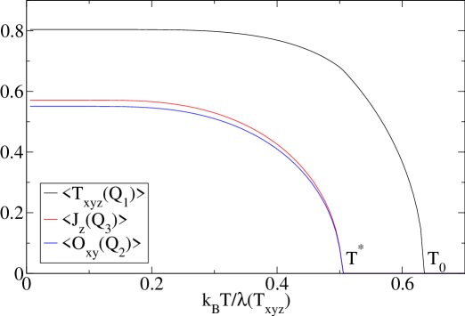
Figure 6: Mean field solution for two consecutive phase transitions. Following the onset of staggered ${\cal T}_{xyz}$ octupolar order, the coupled quadrupolar ${\cal O}_{xy}({\bf Q}_{2})$ and dipolar $J_{z}({\bf Q}_{3})$ order parameters appear at a lower critical temperature (the parameters are given in the text. Note the break in the slope of $\langle{\cal T}_{xyz}({\bf Q}_{1})\rangle$ at $T=T^{*}$. This anomaly will be clearly seen in Fig. 7 (right).

For the order parameters appearing at $T^{*}$, any of the pairs in (9) could be chosen. For the moment, we arbitrarily pick ${\cal O}_{xy}$ and $J_{z}$.

Ordering is possible by the induced moment mechanism in spite of crystal field splittings, but its nature is basically the same as it would be for three degenerate singlets. We introduced three mean field couplings: $\lambda({\cal T}_{xyz})$, $\lambda({\cal O}_{xy})$, and $\lambda(J_{z})$, and solved the self-consistency equations for the three order parameters.

  

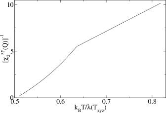
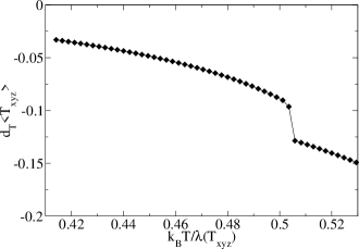
Figure 7: Left: The temperature dependence of the inverse staggered quadrupolar susceptibility. Right: the discontinuity in the temperature derivative of the octupolar moment at $T^{*}$.

Typical results are shown in Fig. 6. The onset of ${\cal T}_{xyz}$ octupolar order at $T_{0}=0.645$ is followed by the ordering of ${\cal O}_{xy}$ and $J_{z}$ at $T^{*}\approx 0.495$. To bring out the contrast between the complementary parameters ${\cal O}_{xy}$ and $J_{z}$, we used the parameter set $\Delta_{21}=1$ as the energy unit, $\Delta_{41}/\Delta_{21}=2$, $\lambda({\cal O}_{xy})=\lambda(J_{z})$, $\lambda(J_{z})/\Delta_{21}=10$, and $\lambda({\cal T}_{xyz})/\Delta_{21}=17$.

The second step of ordering is assisted by the pre-existing octupolar order. This can be seen in the susceptibility plot Fig. 7 (left). We have chosen the quadrupolar susceptibility which belongs to the ordering degree of freedom ${\cal O}_{xy}({\bf Q}_{2})$. The high-temperature susceptibility extrapolates to a lower quadrupolar ordering temperature than the behavior calculated within the octupolar phase. An alternative argument is based on the Landau expansion (we drop the Qs)

$${\cal F} = a_{\rm oct}(T-T_{0}){\cal T}^{2}+b_{\rm oct}{\cal T}^{4}+a_{\rm quad}(T-T_{1})({\cal O}^{2}+J^{2})$$ (14)

$$+b_{\rm quad}({\cal O}^{4}+J^{4})+e{\cal T}^{2}({\cal O}^{2}+J^{2})+f{\cal T}{\cal O}J$$

The last term corresponds to (13). Whatever the sign of $f$, the sign of ${\cal O}J$ can be chosen so that the term lowers the free energy, and enhances the lower critical temperature from $T_{1}$ to $T^{*}$, as observed.

The octupolar order responds to the onset of quadrupolar-dipolar order by a change of the slope of the temperature dependence (Fig. 7, right).

We emphasize that we did not make any attempt to fine-tune our mean field parameters. If we plotted the specific heat, it would show two lambda-anomalies, in conflict with the experiments known to us. We think that until further experiments are done, it would be pointless to refine our calculation.

5 Conclusion

We studied possible sequences of symmetry breaking transitions in tetragonal $f^{2}$ systems. Assuming that octupolar order sets in first, the next transition may lead to mixed dipole–quadrupole, quadrupole–triakontadipole, or octupole–hexadecapole order. There is an interesting similarity to the recent NQR results by Saitoh et al[1] but we feel that any detailed comparison would be premature.

Appendix A

The off-diagonal multipoles in basis (10-12) are

$$J_{z}=4\sqrt{2}b\left(\begin{array}[]{ccc}0&-i&0\\ i&0&0\\ 0&0&0\end{array}\right)\\ {\mbox{\ \ \ \ \ \ }}{\cal O}_{2}^{2}=2\sqrt{7}\left(\begin{array}[]{ccc}0&0&0\\ 0&0&1\\ 0&1&0\end{array}\right)\\$$ (15)

$${\cal O}_{xy}=(-2\sqrt{14}b+6\sqrt{5-10b^{2}})\left(\begin{array}[]{ccc}0&0&1\\ 0&0&0\\ 1&0&0\end{array}\right)\\$$ (16)

$${\cal T}_{z}^{\beta}=3\sqrt{3}(\sqrt{70}b+5\sqrt{1-2b^{2}})\left(\begin{array}[]{ccc}0&0&-i\\ 0&0&0\\ i&0&0\end{array}\right)\\$$ (17)

$${\cal T}_{xyz}=3\sqrt{105}\left(\begin{array}[]{ccc}0&0&0\\ 0&0&-i\\ 0&i&0\end{array}\right)\\ {\mbox{\ \ \ \ \ \ }}{\cal H}_{1}=3\sqrt{35-70b^{2}}\left(\begin{array}[]{ccc}0&1&0\\ 1&0&0\\ 0&0&0\end{array}\right)$$ (18)

All the matrix elements of the triakontadipole operator ${\overline{J_{x}J_{y}J_{z}(J_{x}^{2}-J_{y}^{2})}}$ vanish in this subspace.

References

- [1] S. Saitoh, S. Takagi, M. Yokoyama, and H. Amitsuka, J. Phys. Soc. Jpn. 74 (2005), 2209.
- [2] A. Kiss and P. Fazekas, Phys. Rev. B 71 (2005), 054415.
- [3] ORBITAL2001: Proc. Int. Conf. on Strongly Correlated Electrons with Orbital Degrees of Freedom , J. Phys. Soc. Jpn. 71, Suppl. (2002).
- [4] ASR2002: Advances in the physics of -electron systems, Special Issue of J. Phys.: Condens. Matter 15(28), (2003).
- [5] P. Santini, R. Lémanski, and P. Erdős, Advan. Phys. 48 (1999), 537.
- [6] J. Jensen and A.R. Mackintosh: Rare Earth Magnetism, Clarendon Press, Oxford, 1991.
- [7] F.J. Ohkawa, J. Phys. Soc. Jpn. 52 (1983), 3897 ; 54 (1985), 3909.
- [8] R. Shiina, H. Shiba, and P. Thalmeier: J. Phys. Soc. Jpn. 66 (1997), 1741.
- [9] J.M. Fournier et al., Phys. Rev. B 43 (1991), 1142.
- [10] H. Kusunose and Y. Kuramoto, J. Phys. Soc. Jpn. 70 (2001), 3076.
- [11] H. Shiina, J. Phys. Soc. Jpn. 71, Supplement, p. 56 (2002).
- [12] A. Kiss and P. Fazekas, J. Phys.: Condens. Matter,15 (2003), S2109.
- [13] R. Shiina, J. Phys. Soc. Jpn. 73 (2004), 2257.
- [14] P. Santini and G. Amoretti, Phys. Rev. Lett. 85 (2000), 2188.
- [15] L.I. Korovin and E.K. Kudinov, Fiz. Tverd. Tela 15 (1973), 1228; 16 (1974), 2654.
- [16] F. Vernay, K. Penc, P. Fazekas, and F. Mila, Phys. Rev. B 70 (2004), 014428.
- [17] A. Takahashi and H. Shiba, J. Phys. Soc. Jpn. 69 (2000), 3328.
- [18] J. van den Brink and D. Khomskii, Phys. Rev. B 63 (2001), 140416.
- [19] R. Maezono and N. Nagaosa: Phys. Rev. B 62 (2000), 011576.
- [20] H. Kusunose and Y. Kuramoto, J. Phys. Soc. Jpn. 70 (2001), 1751.
- [21] K. Kubo and Y. Kuramoto, J. Phys. Soc. Jpn. 72 (2003), 1859; 73 (2004), 216.
- [22] J.A. Paixao et al, Phys. Rev. Lett. 89 (2002), 187292; R. Caciuffo et al., J. of Phys.: Condens. Matter 15 (2003) S2287.
- [23] A. Kiss and P. Fazekas, Phys. Rev. B 68 (2003), 174425.
- [24] K. Kubo and T. Hotta, Phys. Rev. B 71 (2005), 140404(R).
- [25] O. Sakai, R. Shiina, and H. Shiba, J. Phys. Soc. Japan 74 (2005), 457.
- [26] T. Sakakibara et al, J. Phys. Soc. Japan 69, Suppl. A (2000), 25.
- [27] O.O. Bernal et al, Phys. Rev. Lett. 87 (2001), 196402.
- [28] A. Amato et al, J. of Phys.: Condens. Matter 16 (2004), S4403.
- [29] K. Hiebl, C. Horvath, P. Rogl, and M.J. Sienko, J. Magn. Magn. Mater. 37 (1983), 287.
- [30] W. Schlabitz et al, Z. Phys. B 62 (1986), 171.
- [31] C. Broholm et al., Phys. Rev. Lett. 38 (1987), 1467.
- [32] P. Chandra, P. Coleman, J.A. Mydosh and V. Tripathi, Nature (London) 417 (2002), 831.
- [33] A. Virosztek, K. Maki, and B. Dóra, Int. J. Modern Phys. B 16 (2002), 1667.
- [34] V.P. Mineev and M.E. Zhitomirsky, Phys. Rev. B 72 (2005), 014432.
- [35] C.M. Varma and L. Zhu, cond-mat/0502344.
- [36] B. Coqblin and J.R. Schrieffer, Phys. Rev. 185 (1969), 847.
- [37] H. Shiba and P. Fazekas, Progr. Theor. Phys. Suppl. 101 (1990), 403 .
- [38] S. Doniach, Physica B 91 (1977), 231; P. Coleman and N. Andrei, J. Phys.: Condens. Matter 1 (1989), 4057; S. Doniach and P. Fazekas, Phil. Mag. B 65 (1992), 1171; P. Coleman, cond-mat/0206003.
- [39] J. Otsuki, H. Kusunose, and Y. Kuramoto, J. Phys. Soc. Japan 74 (2005), 200 .
- [40] S. Watanabe and Y. Kuramoto, Z. Phys. B 104 (1997), 535; S. Watanabe, Y. Kuramoto, T. Nishino, and N. Shibata, J. Phys. Soc. Japan 68 (1999), 159.
- [41] As for the system PrFe4P12 which shows Kondo behavior in its high-temperature phase, but at low temperatures, a localized electron model of the antiferro-quadrupolar order is satisfactory (Ref. [12], A. Kiss and Y. Kuramoto, cond-mat/0504014).
- [42] D.F. Agterberg and M.B. Walker, Phys. Rev. B 50 (1994), 563.
- [43] M.B. Walker et al, Phys. Rev. Lett. 71 (1993), 2630.
- [44] T. Inui, Y. Tanabe, and Y. Onodera, Group Theory and Its Applications in Physics, Springer Series in Solid-State Sciences 78 (Springer-Verlag, Berlin, 1990).
- [45] K. Matsuda et al, Phys. Rev. Lett. 87 (2001), 087203.
- [46] H. Amitsuka and M. Yokoyama, Physica B 329-333 (2003), 452.
- [47] H. Amitsuka et al., Physica B 326 (2003), 418.
- [48] N. Shah, P. Chandra, P. Coleman, and J.A. Mydosh, Phys. Rev. B 61 (2000), 564.
- [49] We may observe that A) is difficult to satisfy since in Table 1., is the only operator with symmetry. Naturally, Table 1. is not exhaustive, and more complicated operators like plaquette dipoles, may have the same symmetry as .
- [50] Recent high-field experiments are interpreted as evidence that hidden order breaks time reversal invariance but has the same symmetry as antiferromagnetism. See F. Bourdarot et al., Physica B 359-361 (2005), 986.
- [51] A.P. Ramirez et al, Phys. Rev. Lett. 68 (1992), 2680.
- [52] P. Santini, Phys. Rev. B 57 (1998), 5191.
- [53] M. Yokoyama et al., cond-mat/0311199 (2003).
- [54] T. Nagao and J. Igarashi, J. Phys. Soc. Jpn. 74 (2005), 765.
- [55] M. Jaime et al, Phys. Rev. Lett. 89 (2002), 287201; K.H. Kim et al, Phys. Rev. Lett. 91 (2003), 256401; A. Suslov et al., Phys. Rev. B 68 (2003), 020406.
- [56] M. Kohgi et al., J. Phys. Soc. Japan 72 (2003), 1002.
- [57] F.J. Ohkawa and H. Shimizu, J. of Phys.: Condens. Matter 11 (1991), L519.