Monte Carlo study of half–magnetization plateau and magnetic phase diagram in pyrochlore antiferromagnetic Heisenberg model

Abstract

The antiferromagnetic Heisenberg model on a pyrochlore lattice under external magnetic field is studied by classical Monte Carlo simulation. The model includes bilinear and biquadratic interactions; the latter effectively describes the coupling to lattice distortions. The magnetization process shows a half–magnetization plateau at low temperatures, accompanied with strong suppression of the magnetic susceptibility. Temperature dependence of the plateau behavior is clarified. Finite–temperature phase diagram under the magnetic field is determined. The results are compared with recent experimental results in chromium spinel oxides.

url]http://www.riken.jp/lab-www/cond-mat-theory/
motome/index-e.html

1 Introduction

Geometrically frustrated magnetism is one of the long–standing issues in condensed–matter physics. Geometrical frustration leads to nearly–degenerate ground–state manifolds of a large number of different spin configurations. The degeneracy may yield nontrivial phenomena, such as spin liquid states and glassy states [1, 2]. Because of the small energy scale of the nearly–degenerate manifolds, a tiny perturbation can be relevant to lift the degeneracy in these systems. For example, quantum or thermal fluctuations can give rise to non–trivial phase transitions in applied magnetic field, leading to a plateau or jump in the magnetization.

Pyrochlore lattice is a typical example of the geometrically–frustrated structures; it consists of a three–dimensional network of corner–sharing tetrahedra as shown in Fig. 1. Pyrochlore lattice is highly frustrated: Classical antiferromagnetic Heisenberg models with only nearest–neighbor interactions do not show any long–range ordering down to the lowest temperature $T=0$ [3, 4]. The situation is similar in the $S=1/2$ quantum spin model as well [5, 6]. Effects of several perturbations on the highly–degenerate states have been discussed, such as quantum fluctuations [6, 7], further–neighbor interactions [3, 8], spin–lattice coupling [9, 10] and Dzyaloshinsky–Moriya interaction [11].

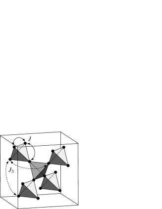
Figure 1: Cubic unit cell of the pyrochlore lattice. Nearest–neighbor exchanges $J$ and third–neighbor exchanges $J_{3}$ are shown, which are incorporated in our model for the MC calculations. See Sec. 2 for the details.

Pyrochlore magents are found in many real compounds. Most typically, so–called $B$ spinel oxides $AB_{2}$O₄ have the pyrochlore structure of the magnetic $B$ cations. Among the $B$ spinels, chromium spinel oxides $A$Cr₂O₄ with nonmagnetic $A$ cations have attracted much interests recently [12]. In these compounds, each Cr³⁺ cation has three $d$ electrons in three–fold $t_{2g}$ levels, which constitute the $S=3/2$ localized spin by the Hund’s–rule coupling. Hence, $t_{2g}$ levels are half–filled and there is no orbital degree of freedom in contrast to the compounds with $B$=V [13, 14] or Ti [15]. Therefore, the Cr spinels provide simple $S=3/2$ spin systems where detailed comparisons between experimental and theoretical studies can be made rather straightforwardly.

Recently, the chromium spinel oxides have been studied by applying external magnetic field [16]. Surprisingly, it was revealed that some of them exhibit a half–magnetization plateau in a very wide range of the magnetic field. For instance, the magnetization process of HgCr₂O₄ shows a plateau from 10 Tesla to 27 Tesla.

The spin–lattice coupling as a possible mechanism of the plateau formation in the Cr spinels has been proposed and studied theoretically [17]. The spin–lattice coupling leads to effective biquadratic interaction between spins. The $T=0$ study of the classical Heisenberg model on the pyrochlore lattice has revealed that for finite biquadratic interactions, the model exhibits a collinear state at intermediate magnetic–field regime, in which each tetrahedron has 3–up and 1–down spin configuration. This collinear state gives rise to a stable half–magnetization plateau. The magnetization process is favorably compared with the experimental results.

Main purpose of the present study is to investigate the plateau problem in the pyrochlore Heisenberg model at finite temperatures in order to make further comparisons with the experimental results. We will employ Monte Carlo (MC) calculations to clarify effects of thermal fluctuations, which are neglected in the previous $T=0$ study and may play a crucial role in the frustrated systems. We will show the temperature dependences of the magnetization curve and the magnetic susceptibility under the external magnetic field, and summarize the finite–temperature phase diagram. We will compare the results with the experimental data.

This paper is organized as follows. In Sec. 2, we introduce the bilinear–biquadratic Heisenberg model. MC method is also described. In Sec. 3, we show numerical results in comparison with the previous $T=0$ results and the experimental data. Section 4 is devoted to summary and concluding remarks.

2 Model and Method

Our starting point is a classical Heisenberg model with the spin–lattice coupling of spin–Peierls type on the pyrochlore lattice under the external magnetic field [17]. The Hamiltonian is given in the form

$$H = \sum_{ij}\Big{[}J_{ij}(1-\alpha\rho_{ij})\mbox{\boldmath$S$}_{i}\cdot\mbox{\boldmath$S$}_{j}+\frac{K_{ij}}{2}\rho_{ij}^{2}\Big{]}$$ (1)

$$- \sum_{i}\mbox{\boldmath$h$}\cdot\mbox{\boldmath$S$}_{i},$$

where $J_{ij}$ is the exchange constant for the spins at the sites $i$ and $j$, $S$ is a classical vector with the modulus $|\mbox{\boldmath$S$}|=1$, $\alpha$ is the spin–lattice coupling constant, $\rho_{ij}$ is the change of the bond length between $i$th and $j$th sites, $K_{ij}$ is the elastic constant for the $ij$ bond, and $h$ is the external magnetic field. This model has been studied at zero magnetic field to describe the low–temperature properties of Cr spinel compounds [10].

In Eq. (1), the lattice distortions $\rho_{ij}$ are quadratic, leading to Gaussian integrals in the partition function, and therefore they can be integrated out. In general case, the integration results in a complicated effective spin–Hamiltonian with long–range interactions between spin–bonds. However, assuming four–sublattice long–range ordering, and nearest–neighbor exchange $J$ and elastic coupling $K$ only [17], the effective Hamiltonian for the ordered moments appearing in the resultant partition function is equivalent to

$$H=\sum_{\langle ij\rangle}J\big{\{}\mbox{\boldmath$S$}_{i}\cdot\mbox{\boldmath$S$}_{j}-b(\mbox{\boldmath$S$}_{i}\cdot\mbox{\boldmath$S$}_{j})^{2}\big{\}}-\sum_{i}\mbox{\boldmath$h$}\cdot\mbox{\boldmath$S$}_{i},$$ (2)

where the summation is taken over the nearest-neighbor sites. The second term in Eq. (2) is the biquadratic interaction, with the coupling constant $b=J\alpha^{2}/K.$ Hence, this biquadratic interaction mimics the spin–lattice coupling. It favors a collinear spin configuration as the spin–lattice coupling does since $Jb$ is always positive.

In the present study, for simplicity and as a first step, we neglect all the complications which arise from the lattice distortions apart from the effective bilinear–biquadratic part, and consider the model (2) extended with the third–neighbor exchange $J_{3}$ (as shown in Fig. 1). In particular, we focus on the ferromagnetic $J_{3}<0$ in the following calculations since it stabilizes the simple four–sublattice long–range ordering with the wave vector $\mbox{\boldmath$q$}=0$ [3]. Hereafter, we will set $J=1$ as an energy unit and use the convention of the Boltzmann constant $k_{\rm B}=1$.

We will investigate thermodynamic properties of the model (2) by Monte Carlo (MC) calculations [18]. We employ the Metropolis algorithm with local spin updates to sample spin configurations. We typically perform $10^{5}$ MC samplings for measurements after $2\times 10^{4}$ steps for thermalization. The measurements are performed in every $N_{\rm int}$–times MC update, and we typically take $N_{\rm int}=2$. Results are divided into five bins to estimate statistical errors by variance of average values in the bins. We have checked the convergence and ergodicity of the results by comparing those for different initial spin configurations. The system sizes in the present work are up to $L=8$, where $L$ is the linear dimension of the system measured in the cubic units shown in Fig. 1, i.e., the total number of spins $N$ is given by $L^{3}\times 16$.

3 Results and Discussion

First, we show the magnetic properties of the model. Figure 2 shows the magnetic–field dependences of the magnetization and the uniform magnetic susceptibility at different temperatures for $J_{3}=-0.05$ and $b=0.1$. The magnetization is defined as

$$m=\langle M_{\rm tot}\rangle=\Big{\langle}\big{|}\sum_{i}\mbox{\boldmath$S$}_{i}\big{|}/N\Big{\rangle},$$ (3)

and the susceptibility is measured by

$$\chi=N\big{(}\langle M_{\rm tot}^{2}\rangle-\langle M_{\rm tot}\rangle^{2}\big{)}/T,$$ (4)

where the brackets denote the thermal average. We show the data for $L=8$ since there is no significant system size dependence in the range of parameters investigated.

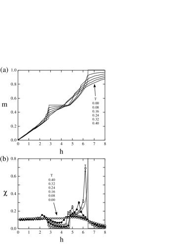
Figure 2: Monte Carlo data at finite temperatures of the magnetic–field dependences of (a) the magnetization and (b) the uniform susceptibility for $J_{3}=-0.05$ and $b=0.1$. The lines are guides for the eyes. The bold gray curves show the results at $T=0$ [17].

As shown in Fig. 2, at low temperatures, the magnetization shows a clear plateau feature at around the half magnetization $m=1/2$. At the same time, the susceptibility exhibits a sharp dip in the corresponding range of the magnetic field. The results indicate that the plateau is stable and survives up to $T\sim 0.3J$ for the present parameters.

Next, we examine the phase diagram under the magnetic field. Following Ref. [17], we measured the order parameters in the form

$$\lambda_{\nu}=\sum_{\rm tetra}\sum_{\alpha}\Lambda_{\nu,\alpha}^{2}/N_{\rm tetra},$$ (5)

where the first summation is taken over all the $N_{\rm tetra}=N/4$ independent tetrahedra (up–pointing ones in the [111] direction). The index $\nu$ denotes the irreducible representations (irreps) of the tetrahedral symmetry group $T_{d}$, i.e., $\nu=\{A_{1},E,T_{2}\}$, and the summation on $\alpha$ is taken over members of a given irreps. The irreps $\Lambda_{\nu,\alpha}$ are given by $\rho_{\nu,\alpha}$ in Eq. (4) in Ref. [17] with replacing $\rho_{i,j}$ by $\mbox{\boldmath$S$}_{i}\cdot\mbox{\boldmath$S$}_{j}$ on r.h.s of the equation.

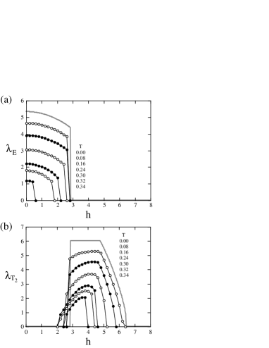
Figure 3: Monte Carlo data of the order parameters with (a) $E$ symmetry and (b) $T_{2}$ symmetry for $J_{3}=-0.05$ and $b=0.1$. The lines are guides for the eyes. The bold gray curves show the results at $T=0$ [17].

Figure 3 shows the MC results for the order parameters with the symmetry $E$ and $T_{2}$. At low temperatures, $\lambda_{E}$ becomes finite in the low–field regime $h\sim 0$. This corresponds to a coplanar long–range ordering with tetragonal symmetry. On the other hand, $\lambda_{T_{2}}$ becomes finite in a middle range of the magnetic field $h\sim 4$, indicating a 3–up 1–down type long–range ordering with trigonal symmetry. Typical spin configurations are shown in Fig. 4.

The $\lambda_{T_{2}}$ order parameter alone, however, does not differentiate between the collinear phase which exhibits the magnetization plateau in Fig. 2 and the non–collinear but coplanar spin–canting phase as shown in the phase diagram at $T=0$ [17]. To identify these phases, we have examined the collinearity and the coplanarity of the spins by calculating the so–called nematic order parameters, and successfully determined the phase boundary between the two phases at finite temperatures [19]. We note that the obtained collinear–coplanar phase boundary corresponds to the shoulder–like feature in the susceptibility at $h\sim 4-5$ in Fig. 2 (b).

Figure 4 summarizes the MC phase diagram for $J_{3}=-0.05$ and $b=0.1$, determined from the data for the system sizes $L=4,6$ and $8$. All the phase transitions are of first order, and the phase boundaries smoothly extrapolate the zero–temperature theoretical values. In addition to the already discussed three ordered phases — the $E$ phase, the collinear $T_{2}$ phase, the spin–canted $T_{2}$ phase — at high temperatures there is the disordered paramagnetic phase. In the figure we also show the typical four–sublattice spin configurations on the tetrahedron for the three ordered phases. The plateau phase is robust against finite–temperature fluctuations, and survives up to even slightly higher temperature than the critical temperature at zero magnetic field.

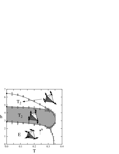
Figure 4: Monte Carlo phase diagram for $J_{3}=-0.05$ and $b=0.1$ Symmetry and typical spin configuration in the tetrahedron are shown for each phase. The shaded area denotes the half–magnetization plateau phase. Filled symbols are the $T=0$ results [17]. The curves for the phase boundaries are guides for the eyes.

The present MC results can be compared favorably with the recent experimental results in Cr spinel compounds such as CdCr₂O₄ and HgCr₂O₄. In particular, the magnetization process in the HgCr₂O₄ has been measured up to the saturation field and the entire phase diagram has been determined [16]. Our MC results in Figs. 2 and 4 give a qualitative description of the experimental results. More quantitative comparison including a fine tuning of the model parameters will be reported elsewhere [19].

4 Summary and Concluding Remarks

To summarize, we have investigated the magnetic properties at finite temperatures of the antiferromagnetic Heisenberg model on the pyrochlore lattice by Monte Carlo calculations. In addition to the ordinary bilinear exchange interaction, our model includes the biquadratic interaction as an effective term describing the coupling of the spins to lattice distortions. By applying magnetic field, we have shown that the model exhibits a stable half–magnetization plateau in a considerable range of temperatures. The results show good agreement with recent experimental results in Cr spinel oxides.

Our study indicates that the spin–lattice coupling plays a dominant role in stabilizing the half–magnetization plateau in Cr spinel oxides. However, we note that other additional elements are indispensable to understand the properties of real compounds in more detail. For instance, at zero magnetic field, recent neutron experiments have found that the spin ordering in the low–temperature phase is complicated, compound–dependent, and incommensurate [20]. To account for such effects, further studies of more realistic Hamiltonians are needed, which would include, e.g., longer–range exchange interactions.

Our further calculations for the model (2) suggest an interesting phenomenon when we weaken the strength of the biquadratic interaction $b$. For small values of $b$, the width (along the $h$ axis) of the plateau phase grows with the temperature. This clearly implies that thermal fluctuations also stabilize the plateau phase. This tendency becomes conspicuous as $b$ decreases, opening a route toward the so–called order–from–disorder phenomenon [21]. This interesting issue will be discussed elsewhere [22].

Finally, our model is defined for classical spins although the real compounds have $S=3/2$ quantum spins. We have also studied the quantum spin problem by spin–wave analysis, and found that, as expected, the plateau state has a finite spin gap. The details of the spin excitation spectrum will also be discussed elsewhere [23].

References

- [1] For instance, see Magnetic System with Competing Interaction, ed. by H.T. Diep (World Scientific Publishing Co., 1994).
- [2] R. Liebmann, Statistical mechanics of periodic frustrated Ising systems (Springer–Verlag, Berlin, Tokyo, 1986).
- [3] J.N. Reimers, A.J. Berlinsky, and A.–C. Shi, Phys. Rev. B 43, 865 (1991); J.N. Reimers, ibid. 45, 7287 (1992).
- [4] R. Moessner and J.T. Chalker, Phys. Rev. Lett. 80, 2929 (1998); Phys. Rev. B 58, 12049 (1998).
- [5] B. Canals and C. Lacroix, Phys. Rev. B 61, 1149 (2000).
- [6] A.B. Harris, A.J. Berlinsky, and C. Bruder, J. Appl. Phys. 69, 5200 (1991).
- [7] H. Tsunetsugu, Phys. Rev. B 65, 024415 (2001).
- [8] J.N. Reimers, J.E. Greedan, and M. Björgvinsson, Phys. Rev. B 45, 7295 (1992).
- [9] Y. Yamashita and K. Ueda, Phys. Rev. Lett. 85, 4960 (2000).
- [10] O. Tchernyshyov, R. Moessner, and S.L. Sondhi, Phys. Rev. Lett. 88, 067203 (2002); Phys. Rev. B 66, 064403 (2002).
- [11] M. Elhajal, B. Canals, R. Sunyer, and C. Lacroix, Phys. Rev. B 71, 094420 (2005).
- [12] S.–H. Lee, C. Broholm, T.H. Kim, W. Ratcliff II, and S.–W. Cheong, Phys. Rev. Lett. 84, 3718 (2000); S.–H. Lee, C. Broholm, W. Ratcliff, G. Gasparovic, Q. Huang, T.H. Kim and S.–W. Cheong, Nature 418, 856 (2002).
- [13] H. Tsunetsugu and Y. Motome, Phys. Rev. B 68, 060405(R) (2003); Y. Motome and H. Tsunetsugu, ibid. 70, 184427 (2004).
- [14] O. Tchernyshyov, Phys. Rev. Lett. 93, 157206 (2004).
- [15] S. Di Matteo, G. Jackeli, C. Lacroix, and N.B. Perkins, Phys. Rev. Lett. 93, 077208 (2004)
- [16] H. Ueda, H.A. Katori, H. Mitamura, T. Goto, and T. Takagi, Phys. Rev. Lett. 94, 047202 (2005); H. Ueda, H. Mitamura, T. Goto, and Y. Ueda, unpublished.
- [17] K. Penc, N. Shannon, and H. Shiba, Phys. Rev. Lett. 93, 197203 (2004).
- [18] Y. Motome, H. Tsunetsugu, T. Hikihara, N. Shannon, and K. Penc, unpublished.
- [19] K. Penc, N. Shannon, and Y. Motome unpublished.
- [20] J.–H. Chung et al., unpublished.
- [21] J. Villain, J. Phys. C: Solid State Phys. 10, 1717 (1977); Z Phys. B 33, 31 (1979).
- [22] Y. Motome, K. Penc, and N. Shannon, unpublished.
- [23] N. Shannon, Y. Motome, and, K. Penc, unpublished.