A Single Atom Mirror for 1D Atomic Lattice Gases

Abstract

We propose a scheme utilizing quantum interference to control the transport of atoms in a 1D optical lattice by a single impurity atom. The two internal state of the impurity represent a spin-1/2 (qubit), which in one spin state is perfectly transparent to the lattice gas, and in the other spin state acts as a single atom mirror, confining the lattice gas. This allows to “amplify” the state of the qubit, and provides a single-shot quantum non-demolition measurement of the state of the qubit. We derive exact analytical expression for the scattering of a single atom by the impurity, and give approximate expressions for the dynamics a gas of many interacting bosonic of fermionic atoms.

I Introduction

One of the fundamental models in quantum optics is the interaction of a spin-$1/2$ system with a bosonic mode Cohen . The most prominent example is cavity quantum electrodynamics (CQED), where a two level atom interacts with a single mode of the radiation field in a high-Q cavity. CQED has been the topic of a series of seminal experiments both in the microwave and optical regime, demonstrating quantum control on the level of single atoms and photons in an open quantum system Kimble ; Haroche ; Rempe ; Walther .

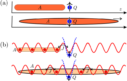
Figure 1: (a) A spin 1/2 impurity $Q$ used as a switch: in one spin state it is transparent to the probe atoms $A$, but in the other it acts as a single atom mirror. (b) Implementation of the SAT: The impurity atom $Q$ and the probe atoms $A$ are trapped separately in state-dependent 1D optical lattices. The probe atoms $A$ initially are in a Mott insulating state.

In the present paper we will consider a system with the same basic ingredients, however in the context of cold atoms and quantum degenerate gases. The key feature of these systems is there controllability and weak decoherence. In particular we employ two aspects of control, the confinement of atoms in optical lattices JakschZollerReview ; Greiner ; Mandel ; Stoeferle and (magnetic or optical) Feshbach resonances as a way to manipulate atomic interactions Bolda ; Julienne ; Holland ; Theis . According to the setup described in Fig. 1(a) we will study the dynamics of an atomic quantum gas in 1D (with a single internal atomic state), representing bosonic or fermionic “modes”, controlled by an atomic spin-1/2 impurity. The quantum gas is confined by tight trapping potentials (e.g. an optical or magnetic trap), so that only the motional degrees along the $z$-axis in Fig. 1(a) are relevant. In the $z$-direction the motion is confined to the left by a trapping potential (e.g. a blue sheet of light), while the atomic impurity restricts the motion of the gas to the right due to collisional interactions of the quantum gas with the impurity. The atom representing the impurity can, for example, be a different atomic species in a tight trapping potential, a configuration discussed in Refs. Recati ; Raizen as an atomic quantum dot ($0$D system). Thus the impurity atom plays the role of “single atom mirror” confining the quantum gas in an “atomic cavity”.

In our model system the impurity atom is an internal two level system, which we write as an effective spin-1/2. In the following we will also interpret this two-level system as a qubit with two logical states $|0\rangle=|\downarrow\rangle$ and $|1\rangle=|\uparrow\rangle$. Cold atom collision physics allows for a situation where the collisional properties (scattering length) of the impurity atom and atoms in the quantum gas are spin-dependent. As illustrated in Fig. 1(a), we assume that in one spin state, say $|\downarrow\rangle$, the single impurity atom is completely transparent for the quantum gas, i.e. the gas will leak out through the “mirror”. In contrast, in the other spin state the mirror atom is “highly reflective” confining the gas. For an impurity atom (qubit) initially prepared in a spin superposition

$$|\psi_{Q}(t=0)\rangle=\alpha_{\uparrow}|\uparrow\rangle+\alpha_{\downarrow}|\downarrow\rangle$$

the combined system at a time $t$ will be in a macroscopic superposition state

$$|\Psi(t)\rangle=\alpha_{\uparrow}|\uparrow\rangle|\phi_{\uparrow}(t)\rangle+\alpha_{\downarrow}|\downarrow\rangle|\phi_{\downarrow}(t)\rangle.$$ (1)

with $|\phi_{\sigma}(t)\rangle$ many body wave functions of the gas atoms. Thus $|\Psi(t)\rangle$ represents a Schrödinger cat state of two entangled quantum phases of gas atoms, the first one corresponding to gas confined by the mirror (Fig. 1(a) upper figure) and the second one to the expanding gas (Fig. 1(a) lower figure). The entanglement of the spin with a macroscopic number of atoms can be interpreted as a macroscopic quantum gate, as explained in Fig. 2), implementing a quantum nondemolition interaction (QND) qnd . In this sense the setup represents a “amplifier” of the state of the qubit. This situation is reminiscent of a Single Electron Transistor (SET) in mesoscopic physics set , and has stimulated the name Single Atom Transistor (SAT) for the setup Fig. 1(a) in Ref. Micheli , with the essential difference that the dynamics underlying (1) is completely coherent. We finally remark that this setup also allows for a single shot QND measurement of the impurity atom (qubit) by observing in a single experiment the distinct properties of the $|\phi_{\downarrow}(t)\rangle$ or $|\phi_{\uparrow}(t)\rangle$ quantum phases.

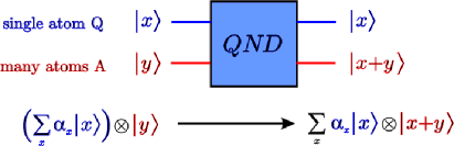
Figure 2: The single atom mirror as a macroscopic quantum gate. The qubit $Q$ entangles two distinguishable macroscopic phase of the probe atoms $A$ and provides for a quantum nondemolition interaction.

As a variant of the configuration of Fig. 1(a) we will consider below in particular the case where the quantum gas is loaded in an optical lattice, as illustrated in Fig. 1(b). In this case the gas could be loaded initially, for example, in a Mott insulating state, i.e. where large repulsion of the gas atom leads to a filling of the lattice sites with exactly one atom per lattice site Jaksch ; Greiner ; Stoeferle . The cat state (1) will thus correspond to a superposition of the Mott phase and the melted Mott phase, i.e. a (quasi-) condensate of atoms obtained by expansion of the atomic gas:

$$|\Psi(t)\rangle=\alpha_{\downarrow}|\downarrow\rangle|\textrm{BEC}\rangle+\alpha_{\uparrow}|\uparrow\rangle|\textrm{Mott}\rangle.$$ (2)

In this case the distinguishing features of the two entangled quantum phases are the observation / non-observation of interference fringes as signatures of the Mott and BEC phase, when the atomic gas in released in a single experiment.

Transport through an impurity is a well studied problem in mesoscopic condensed matter physics Datta ; Mahan ; Levitov ; Cazalilla , which typically focuses on conductance properties of a system attached to leads. In contrast, in the context of cold gases we have a full time-dependent coherent dynamics in an otherwise closed system.

A short summary of the present work including results from numerical studies was presented in Ref. Micheli . In this paper we will present details of our analytical calculations, while we refer to Ref. Daley on a complementary numerical treatment of these problems using time dependent DMRG techniques.

The paper is organized as follows: In Sec. II we introduce the model used for describing the implementation of the Single Atom Mirror using cold atoms in optical lattice. In Sec. III we consider the detailed scattered processes involved in the transport of a single particle through the mirror. We solve exactly the scattering problem in the lattice by integrating the Lippmann-Schwinger Equation (LSE) and discuss the obtained scattering amplitudes and spectrum of the bound states. Finally, in Sec. IV we generalize the discussion to the case of interacting many-systems including the cases of a 1D degenerate Fermi-gas, a 1D quasi-condensate and Tonks gas.

II Model

In this section we introduce the our model system by specifying the Hamiltonian for a 1D lattice gas coupled to an impurity, and we explain the key idea behind our setup. We will start with a discussion of spin-dependent collisions between the gas and the impurity, and then present the central idea of quantum interference as a way to switch atomic transport.

II.1 Effective Spin-Dependent Hamiltonian

We consider the dynamics of a spin-1/2 atomic impurity $Q$ coupled to a 1D quantum gas of either bosonic or fermionic probe atoms $A$. The Hamiltonian for system is split into three parts as

$$H = H_{A}+H_{Q}+H_{AQ}.$$ (3)

Here $H_{Q}$ ($H_{A}$) describes the uncoupled dynamics of the impurity atom $Q$ (the degenerate quantum gas of probe atoms $A$), while $H_{AQ}$ accounts for the interaction between the two atomic species, $Q$ and $A$.

A degenerate quantum gas of bosonic or fermionic atoms $A$ trapped in the lowest band of a 1D optical lattice is well described by a Hubbard model JakschZollerReview

$$H_{A} = \sum_{j}E_{A,j}a_{j}^{\dagger}a_{j}-J\sum_{\langle ij\rangle}a_{i}^{\dagger}a_{j}+\frac{U}{2}\sum_{j}a_{j}^{\dagger}a_{j}^{\dagger}a_{j}a_{j},$$ (4)

where $a_{j}^{\dagger}$ ($a_{j}$) are the creation (annihilation) operators for an atom $A$ on the site $j$, which obey standard commutation (anticommutation) relations for the case of bosonic (fermionic) atoms $A$. Moreover, $E_{A,j}$ account for the shift of the bare energy of an atom localized on the site $j$ in the presence of an external (e.g. magnetic) shallow trap, $J$ is the tunneling matrix element for neighboring sites $\langle ij\rangle$ and $U$ gives the collisional interaction, i.e. the onsite-shift for two atoms $A$ localized within the same well (which would be zero for the case of fermions in the same internal state). Denoting the scattering-length of the atoms $A$ by $a_{s}$, and their mass by $m$, we have $U=4\pi\hbar^{2}a_{s}\int d^{3}r|w_{j}({\bf r})|^{4}/m$, where $w_{j}({\bf r})$ is the Wannier function for a particle localize on the site $j$.

In the present setup we regard the impurity atom $Q$ to be trapped within a tight one-dimensional lattice, as depicted in Fig. 1(b). Therefore, we may restrict ourselves to the lowest trap-state of the $j=0$ well for the internal states $\sigma=\downarrow,\uparrow$, respectively. The uncoupled dynamics of the impurity corresponds to spin-1/2 system, i.e.

$$H_{Q} = \sum_{\sigma}E_{Q,\sigma}|Q_{\sigma}\rangle\langle Q_{\sigma}|,$$ (5)

where $|Q_{\sigma}\rangle$ ($E_{Q,\sigma}$) denotes the state (energy) of the atom $Q$ with spin $\sigma=\downarrow,\uparrow$.

Given the tight trapping of the impurity atom, the interaction of probe and impurity atom is restricted to the site of the impurity, an in general has the form of an effective spin-dependent collisional interaction

$$H_{AQ} = W_{{\rm eff},\uparrow}|\uparrow\rangle\langle\uparrow|a_{0}^{\dagger}a_{0}+W_{{\rm eff},\downarrow}|\downarrow\rangle\langle\downarrow|a_{0}^{\dagger}a_{0},$$ (6)

where $a_{0}^{\dagger}$ ($a_{0}$) is the creation (annihilation) operator for a probe atom on the site of the impurity, $j=0$. Here, $W_{{\rm eff},\sigma}=4\pi\hbar^{2}a_{\sigma}/\mu\int d^{3}r|w_{0}({\bf r})|^{2}|\psi_{Q,\sigma}({\bf r})|$ denotes the effective interaction for a probe atom $A$ and the impurity atom $Q$ in state $\sigma$ in terms of their effective scattering length $a_{\sigma}$ and $\mu$ is the reduced mass for $A$ and $Q$. The effective tunneling rate of a probe atom with energy $E$ through the impurity is then given by $J_{{\rm eff},\sigma}=J^{2}/(E-W_{{\rm eff},\sigma})+{\cal O}(J^{4})$ for the qubit in state $\sigma$. An obvious way to provide for a spin-dependent single atom mirror is to have the effective interaction for one spin state as large as possible ($|W_{{\rm eff},\uparrow}|\gg J$), thus blocking the transport of the probe atoms through the impurity site, while for the other it is effectively not present, ($|W_{{\rm eff},\downarrow}|\ll J$). This can be achieved, for example, by tuning the internal state dependent scattering length $a_{\sigma}$ or by engineering the spin-dependent trapping JakschZollerReview . The quality of the qubit dependent switch then depends on the difference of the moduli of the effective interactions, $|W_{{\rm eff},\uparrow}|-|W_{{\rm eff},\downarrow}|$. Thus the goal an efficient scheme is to make $|W_{{\rm eff},\uparrow}|-|W_{{\rm eff},\downarrow}|$ as large as possible and obtain $|W_{{\rm eff},\uparrow}|\gg J\gg|W_{{\rm eff},\downarrow}|$.

II.2 Controlling the transport by interference

In this section we will show now that with the help of quantum interference we can engineer an effectively infinite (zero) atomic repulsion, $W_{{\rm eff},\uparrow}\rightarrow\infty$ ($W_{{\rm eff},\downarrow}\rightarrow 0$), for the qubit in state $\sigma=\downarrow$ ($\sigma=\uparrow$). This is equivalent to tuning the Feshbach resonance to the point of infinite (zero) scattering length.

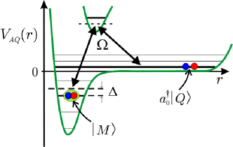
Figure 3: The optical Feshbach setup couples the atomic state $a^{\dagger}_{0}|Q\rangle$ (in a particular motional state quantized by the trap) to a molecular bound state $|M\rangle$ of the Born-Oppenheimer potential $V_{AQ}(r)$ with effective Rabi frequency $\Omega$ and detuning $\Delta$.

The quantum interference mechanism required to engineer the described spin-dependence of $W_{{\rm eff},\sigma}$ is obtained by exploiting the properties of either an optical or a magnetic Feshbach resonance. In the case of an optical Feshbach resonance a Raman laser drives the transitions from the joint state of the two atoms on the impurity site, $a_{0}^{\dagger}|Q_{\sigma}\rangle\equiv|Q_{\sigma}\rangle\otimes a_{0}^{\dagger}|{\rm vac}\rangle$, via an off-resonant excited molecular state back to a bound hetero-nuclear molecular state $|M_{\sigma}\rangle$ in the lowest electronic manifold (see Fig. 3). The Raman processes is described by the effective two-photon Rabi frequency $\Omega_{\sigma}$ and detuning $\Delta_{\sigma}$ for each spin-component $\sigma$. For the case of a magnetic Feshbach resonance, the effective Hamiltonian has the same form, but with $\Omega_{\sigma}$ being the coupling strength between the open and closed channels and $\Delta_{\sigma}$ the detuning of the magnetic field. The Hamiltonian describing the interaction between the probe atoms and the impurity is Holland

$$H_{AQ}=\sum_{\sigma}\Big{[}E_{M,\sigma}|M_{\sigma}\rangle\langle M_{\sigma}|+\Omega_{\sigma}\left(|M_{\sigma}\rangle\langle Q_{\sigma}|a_{0}+{\rm h.c.}\right)$$

$$+W_{Q,\sigma}|Q_{\sigma}\rangle\langle Q_{\sigma}|a_{0}^{\dagger}a_{0}+W_{M,\sigma}|M_{\sigma}\rangle\langle M_{\sigma}|a_{0}^{\dagger}a_{0}\Big{]},$$ (7)

where the bare energy of the molecular bound state is $E_{M,\sigma}=E_{A,0}+E_{Q,\sigma}+\Delta_{\sigma}$. Here the first two terms describe the resonant coupling induced by the Feshbach mechanism, while the last two describe the off-resonant collisions between an atom $A$ and an atom $Q$ (a molecule $M$) in state $\sigma$ by means of their on-site shift $W_{Q,\sigma}$ ($W_{M,\sigma}$) for the impurity site. The Hamiltonian (3) conserves the spin-component of the impurity, $S_{\sigma}\equiv|Q_{\sigma}\rangle\langle Q_{\sigma}|+|M_{\sigma}\rangle\langle M_{\sigma}|$, i.e. $[H,S_{\sigma}]=0$. Therefore, we can consider the dynamics for the two spin components of $Q$ separately, and in the following we will drop the spin index $\sigma$ and choose the reference energy as $E_{A,0}=E_{Q,\sigma}=0$.

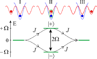
Figure 4: A single atom passes the impurity (I$\rightarrow$III) via the two dressed states (II), $|+\rangle=a^{\dagger}_{0}|Q\rangle+|M\rangle$ and $|-\rangle=a^{\dagger}_{0}|Q\rangle-|M\rangle$ and quantum interference gives rise to an effective tunneling rate $J_{\rm eff}$.

For off-resonant laser driving ($|\Delta|\gg\Omega$), the Feshbach resonance enhances the interaction between $A$ and $Q$ atoms, giving the familiar result $W_{\rm eff}=W_{Q}+\Omega^{2}/\Delta$. However, for resonant driving ($\Delta=0$) the physical mechanism changes, and the effective tunneling $J_{\rm eff}$ of an atom $A$ past the impurity (Fig. 4, $\rm I\rightarrow III$) is blocked by quantum interference. On the impurity site, laser driving mixes the states $a_{0}^{\dagger}|Q\rangle$ and $|M\rangle$, forming two dressed states with energies $E_{\pm}=W_{Q}/2\pm(W_{Q}^{2}/4+\Omega^{2})^{1/2}$ (Fig. 4, II). The two resulting paths for a particle of energy $E$ destructively interfere so that for large $\Omega\gg J$ and $W_{Q}=0$,

$$J_{\rm eff} = -\frac{J^{2}}{E+\Omega}-\frac{J^{2}}{E-\Omega}\rightarrow 0.$$

This is analogous to the interference effect underlying Electromagnetically Induced Transparency (EIT) eit , and is equivalent to having an effective interaction $W_{\rm eff}\rightarrow\infty$. In addition, if we choose $\Delta=\Omega^{2}/W_{Q}$, the paths interfere constructively, screening the background interactions $W_{Q}$ to produce perfect transmission ($W_{\rm eff}\rightarrow 0$). The insensitivity of the interference scheme to losses from the dressed states due to their large detuning has been argued in Ref. Micheli .

III Single particle scattering from an impurity

In this section we will analyze the scattering of a single probe atom $A$ from an impurity atom $Q$. We will formulate the scattering problem, then solve the time-independent and time-dependent Schrödinger Equation, to finally obtain the dynamics of wave-packets in the lattice.

We consider a probe atom $A$ approaching the impurity from the left, as a plain Bloch-wave with quasi-momentum $k$. Hence the state of the system is given by

$$|k\rangle=\left(\frac{a}{2\pi}\right)^{1/2}\sum_{j}e^{ikx_{j}}|j\rangle,$$ (8)

where $|j\rangle=|Q\rangle\otimes a_{j}^{\dagger}|{\rm vac}\rangle$ is the joint state of the atoms $A$ and $Q$, with $A$ ($Q$) localized in the lowest vibrational state of the well $j$ (the impurity well $j=0$) and $a$ is the lattice spacing.

The free evolution of the system is given by the hopping of the atoms $A$ between neighboring sites at the tunneling rate $J$, whereas the composite molecule $M$ is detuned by $\Delta$ from the threshold for the joint state of $A$ and $Q$. Thus, with $E_{k}=-2J\cos ka$ being the energy of a Bloch-wave in the first Bloch-band with quasi-momentum $k$, we have

$$H_{0} = -J\sum_{j}\left(|j+1\rangle\langle j|+\mathrm{h.c.}\right)+\Delta|M\rangle\langle M|$$ (9)

$$= \int_{-\pi/a}^{\pi/a}dkE_{k}|k\rangle\langle k|+\Delta|M\rangle\langle M|,$$

where $|M\rangle$ denotes the molecular bound state localized on the impurity site. From Eq. (9) we obtain the propagation of the incoming plane wave $|k\rangle$ at group-velocity $v_{k}=\partial E_{k}/\partial k=2Ja\sin ka$ in the first Bloch band.

Due to the strong confinement of the particles $A$ and $Q$ in the lattices, their interaction is restricted to the impurity site. There, their bare interaction induces an on-site-shift $W$ for the joint atomic state of $A$ and $Q$ on the impurity ($|0\rangle$). Moreover, the photo-association lasers effectively couple the latter state to the trapped molecular state ($|M\rangle$) at Rabi-frequency $\Omega$, yielding

$$V = W|0\rangle\langle 0|+\Omega\left(|M\rangle\langle 0|+\mathrm{h.c.}\right).$$ (10)

III.1 Scattering solution

The scattering of a particle $A$ with energy $E=E_{k}$ in the first Bloch band by the impurity $Q$ is described by a solution of the Lippmann-Schwinger Equation (LSE). The scattering wave function $|\phi_{+}\rangle$ obeys

$$|\phi_{+}\rangle=|k\rangle+G_{0}(E+i0^{+})V|\phi_{+}\rangle,$$ (11)

with incident plane wave $|k\rangle$ with quasimomentum $k$ ($0<k<\pi/a$), and $G_{0}(z)=1/(z-H_{0})$ the free propagator. Expanding the scattering wave function

$$|\phi_{+}\rangle=\left(\frac{a}{2\pi}\right)^{1/2}\left[\sum_{j}\alpha_{j}|j\rangle+\beta|M\rangle\right]$$ (12)

the amplitudes $\alpha_{j}$ and $\beta$ satisfy

$$\alpha_{j} = e^{ikx_{j}}+\mathcal{G}_{j}(E_{k})\left(W\alpha_{0}+\Omega\beta\right),$$ (13a)

$$\beta = \mathcal{G}_{M}(E_{k})\Omega\alpha_{0}$$ (13b)

with atomic and molecular propagators

$$\mathcal{G}_{j}(E) = \langle j|G_{0}(E+i0^{+})|0\rangle$$

$$\equiv \frac{a}{2\pi}\int_{-\pi/a}^{+\pi/a}dk\frac{e^{ikx_{j}}}{E-E_{k}+i0^{+}}=\frac{e^{ik|x_{j}|}}{iv_{k}/a},$$

$$\mathcal{G}_{M}(E) = \langle M|G_{0}(E+i0^{+})|M\rangle\equiv\frac{1}{E-\Delta+i0^{+}}.$$

Solving Eqs.(13) we find

$$\alpha_{j} = e^{ikx_{j}}+\frac{W_{k}}{iv_{k}/a-W_{k}}e^{ik|x_{j}|},$$ (15a)

$$\beta = \frac{-i\Omega v_{k}/a}{\Omega^{2}+\left(E_{k}-\Delta+i0^{+}\right)\left(W-iv_{k}/a\right)}$$ (15b)

with effective energy dependent interaction

$$W_{k}=W+\frac{\Omega^{2}}{E_{k}-\Delta+i0^{+}},$$ (16)

where we read off the transmission and reflection amplitudes

$$t_{k} = \frac{1}{1+iaW_{k}/v_{k}}$$ (17a)

$$r_{k} = \frac{-1}{1-iv_{k}/aW_{k}},$$ (17b)

respectively.

Note that the presence of the molecular state introduces an effective energy-dependent interaction $W_{k}$. This can be interpreted in terms of an effective atomic scattering length with background scattering length proportional to $W$ and a resonant term, corresponding to an optical Feshbach resonance at energy given by the detuning from the molecular state $\Delta$, and width determined by the Rabi frequency $\Omega$.

The scattering matrix

$$S(E_{k})\mathbb{=}\left(\begin{array}[]{cc}r_{k}&t_{k}\\ t_{k}&r_{k}\end{array}\right)$$ (18)

is unitary, as follows readily from the above expressions (17). This implies $T_{k}+R_{k}\equiv|t_{k}|^{2}+|r_{k}|^{2}=1$. We can assign phase shifts $t_{k}\pm r_{k}=\exp(i\delta_{k}^{\pm})$ for the symmetric and antisymmetric states $|k\rangle\pm|-k\rangle$, $\delta_{k}^{+}=-2\arctan(aW_{k}/v_{k})$ and $\delta_{k}^{-}=0$, respectively, so that $R_{k}=\sin^{2}(\delta_{k}^{+}/2)$.

III.2 Discussion of the Scattering Amplitudes

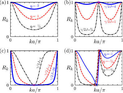
Figure 5: Reflection coefficient $R_{k}$, showing in (a) partial reflection for bare background collisions $W\neq 0$ but $\Omega=0$, i.e. $q_{f}=-1/2,-1,-2$ (dotted, dashed, full line) and $\gamma=E_{R}=0$, (b) complete reflection at $k_{0}=\pi/2a$ for $\gamma/2J=1/4,1,4$ (dotted, dashed, full line) and $E_{R}=q_{f}=0$, cf. $R\approx 1$ for $\gamma/2J=4$ (full line), (c) perfect transmission at $k_{0}=\pi/2a$ for $\gamma/2J=1,4,16$ (dotted, dashed, full line), $q_{f}=-2$ and $E_{R}=\gamma/4$, cf. $R\approx 0$ for $\gamma/2J=16$ (full line), (d) the asymmetry of the Fano-profiles for $q_{f}=-1/4,-1,-4$ (dotted, dashed, full line), $\gamma/2J=1/2$ and $E_{R}=0$.

In the absence of molecular couplings ($\Omega=0$) the on-site interaction $W$ between the B atom and the impurity Q always gives rise to partial reflection and transmission, see Fig. 5a,

$$R_{k}=1-T_{k}=\frac{W^{2}}{W^{2}+4J^{2}\sin^{2}\left(ka\right)}<1.$$ (19)

The significant new feature introduced by the optical Feshbach resonance is that we can achieve essentially complete blocking ($R_{k}=1$) and complete transmission ($T_{k}=1$). We obtain this in the limits $\Omega\gg J$ and $\Delta=0$, and $\Omega\gg J$ and $\Delta=-\Omega^{2}/W$, respectively. Physically, the first case corresponds to tuning to the point of “infinite” scattering length, while the second case corresponds to tuning to the point of “zero” scattering length, respectively.

In the general case the energy dependence of transmission and reflection has the form of a Fano-like profile (see Fig. 5). In the region $|E_{k}|\ll 2J$ we may neglect the dispersion effects, i.e. $v_{k}\approx 2Ja$, and obtain Fano-line-shapes for transmission and reflection as

$$T(\varepsilon) = \frac{1}{1+q_{f}^{2}}\frac{\left(\varepsilon+q_{f}\right)^{2}}{\varepsilon^{2}+1},$$ (20a)

$$R(\varepsilon) = \frac{1}{1+1/q_{f}^{2}}\frac{\left(\varepsilon-1/q_{f}\right)^{2}}{\varepsilon^{2}+1},$$ (20b)

where $\varepsilon\equiv(E-E_{R})/(\gamma/2)$ is the dimensionless energy in units of the resonance width $\gamma$, $E_{R}$ is the resonance energy and $q_{f}$ is the Fano-$q$-parameter. These parameters of the Fano-profile are related to $J,W,\Delta,\Omega$ by

$$\gamma =\frac{4J\Omega^{2}}{W^{2}+4J^{2}},\quad \Omega^{2} =J\gamma\left(q_{f}^{2}+1\right),$$ (21a)

$$E_{R} =\Delta-\frac{W\Omega^{2}}{W^{2}+4J^{2}},\quad \Delta =E_{R}-\frac{q_{f}\gamma}{2},$$ (21b)

$$q_{f} =\frac{-W}{2J},\quad W =-2Jq_{f}.$$ (21c)

For $W=0$ the asymmetry parameter $q_{f}$ vanishes, the reflection profile is symmetric, and for $\Omega>0$ resembles a Breit-Wigner-profile, see Fig 5(b). The maximum $R_{k}=1$ is attained at $\varepsilon=-q_{f}$ ($E_{k}=\Delta$, $|\Delta|<2J$) and has a width $\gamma=\Omega^{2}/J$.

For finite background collisions $q_{f}\neq 0$ ($W\neq 0$) the transmission profile is asymmetric, and shows an additional minimum $R_{k}=0$ at $\varepsilon=-1/q_{f}$ ($E_{k}=\Delta-\Omega^{2}/W=\Delta_{\star}$, $|\Delta_{\star}|<2J$), see Fig 5(c).

Near the edges of the Bloch band, $k_{\pm}=(\pi\mp\pi)/2a$ ($E_{k}=\pm 2J$), transmission and reflection deviate from the Fano line-shape Eq. (20). There the group-velocity $v_{k}\rightarrow 0$ and thus also the transmission $T_{k}$ vanishes, unless the dressed resonance $\Delta_{\star}$ is tuned to respective edge of the Bloch band. The transmission coefficient are given by

$$T_{k{\approx}k_{\pm}}\approx\frac{4J^{2}a^{2}\left(k-k_{\pm}\right)^{2}}{\left[W-\Omega^{2}/\left(\Delta\mp 2J\right)\right]^{2}} \Delta_{\star}\neq\pm 2J,$$ for

$$T_{k{\approx}k_{\pm}}\approx 1-\frac{W^{4}a^{2}\left(k-k_{\pm}\right)^{2}}{2\Omega^{4}} \Delta_{\star}=\pm 2J.$$ for

The reflection coefficient $R_{k}$ as a function of energy $-2J<E_{k}<+2J$ is shown in Fig. 5.

In the absence of molecular coupling, $\gamma=0$ ($\Omega=0$), the reflection is unity at the band-edges, $k=0,\pi/a$, and decreases within the Bloch-band due to the increase of the group-velocity (see Fig.5(a)). The profile is symmetric about the middle of the Bloch band, $k=\pi/2a$, where it attains its minimum,

$$R_{k}=\frac{1}{1+q_{f}^{-2}}=\frac{1}{1+\left(2J/W\right)^{2}}.$$

In the presence of molecular couplings, $\gamma\neq 0$ ($\Omega>0$), and for $E_{R}=q_{f}=0$ the reflection profile is still symmetric about $k=\pi/2a$ (see Fig.5(b)). However, now it approaches its maximum, $R_{k}=1$, at $k=\pi/2a$, and has now two minima at $k\approx\pi/4a$ and $k\approx 3\pi/4a$, given by

$$R_{k}=\frac{1}{1+\left(2J/\gamma\right)^{2}}=\frac{1}{1+\left(\sqrt{2}J/\Omega\right)^{4}}.$$

For $\gamma,q_{f}\neq 0$ we obtain an asymmetric Fano-profile (see Fig.5(d)), which for $|E_{R}+q_{f}\gamma/2|=|\Delta|<2J$ shows complete reflection, $R_{k}=1$, at $\varepsilon=-q_{f}$, while for $|E_{R}-\gamma/2q_{f}|<2J$ one has perfect transmission, $R_{k}=0$, at $\varepsilon=+1/q_{f}$.

The reflective and transmissive resonance are present regardless of the magnitude of $q_{f}$, and their width is $\propto\gamma$. However, for $\gamma\leq 8J|q_{f}+1/q_{f}|$ they may both occur within the physical energy range of the Bloch-band (see Fig.5(d)), while for $\gamma>8J|q_{f}+1/q_{f}|$ only one resonance appears (see Fig.5(b,c)). Thus in the limit $\gamma\gg 8J|q_{f}+1/q_{f}|$ we achieve complete blocking , $R_{k}=1$ for all $k$, by tuning $E_{R}\approx-q_{f}\gamma/2$ (see full-line in Fig.5(b)). Within the same limit we can also efficiently screen any background-interaction $W$ and achieve complete transparency, $T_{k}=1$ for all $k$, by tuning $E_{R}\approx\gamma/2q_{f}$ (see full-line in Fig. 5(c)).

III.3 Interference mechanism

Physically, the features of complete blocking ($R_{k}=0$) and complete transmission ($T_{k}=0$) are induced by an interference mechanism, as the probe atom may tunnel via two interfering paths of dressed atomic + molecular states, as depicted in Fig. 4.

For simplicity we start by elucidating the underlying interference mechanism (present for $\Omega\neq 0$) in the regime of strong coupling, $\Omega^{2}\gg(2J)^{2}+|W\Delta|$. In this regime we can consider the local dynamics within the individual sites, and treat the tunneling $J$ by means of perturbation theory.

To zeroth order in $J$ the Hamiltonian $H$ decouples the dynamics of the individual sites $j$ as

$$H^{(0)}= W|0\rangle\langle 0| +\Omega|0\rangle\langle{M}|+$$

$$+ \Omega|M\rangle\langle 0| +\Delta|M\rangle\langle{M}|.$$ (23)

Outside the impurity ($j\neq 0$) its eigenstates are the joint states of the atoms $A$ and $Q$, $|j\rangle$, with energy $E_{0}=0$, whereas on the impurity ($j=0$) the strong coupling $\Omega$ between the atomic state $|0\rangle$ and the molecular state $|M\rangle$ induces the two states to split into two dressed state $|E_{\pm}\rangle$ of atoms + molecules with energy $E_{\pm}$, see Fig. 4. By diagonalizing the $2\times 2$-matrix in Eq. (23) we obtain the amplitudes and energy of the dressed states as

$$|E_{\pm}\rangle = \left[\frac{1\pm\xi}{2}\right]^{1/2}|0\rangle\pm\left[\frac{1\mp\xi}{2}\right]^{1/2}|M\rangle,$$ (24a)

$$E_{\pm} = \frac{W+\Delta}{2}\pm\left[\Omega^{2}+\left(\frac{W-\Delta}{2}\right)^{2}\right]^{1/2},$$ (24b)

$$\xi = \frac{W-\Delta}{\left[\left(W-\Delta\right)^{2}+4\Omega^{2}\right]^{1/2}},$$ (24c)

where $\xi$ characterizes the asymmetry of the amplitudes, i.e. for $\xi=0$ ($W=\Delta$) the dressing is completely symmetric while for $|\xi|=1$ ($\Omega=0$) the atomic and molecular state decouple. From Eq. (24b) we see that for $\Omega\gg|W\Delta|$ the dressed states are far off-resonant from $E=0$, and hence will be only virtually populated.

The effects of the hopping of the atom $A$ on the $E\approx 0$ modes $|j\neq 0\rangle$ can be accounted by means of an effective Hamiltonian $H_{\rm eff}$. Following Ref. Cohen we obtain the dynamics as a perturbative series in the hopping amplitude $J$, $H_{\rm eff}=H^{(0)}+H^{(1)}+H^{(2)}+\ldots$. To first order in $J$ one obtains

$$H^{(1)} = -J\sum_{j<0}|j\rangle\langle{j-1}|-J\sum_{j>0}|j\rangle\langle{j+1}|+{\rm h.c.}$$ (25)

$$= \sum_{\alpha=L,R}\int dkE_{k}|k_{\alpha}\rangle\langle k_{\alpha}|,$$

where $|k_{L}\rangle$ ($|k_{R}\rangle$) are the Bloch-waves with quasi-momentum $k$ on the left (right) side of the impurity site,

$$|{k_{L,R}}\rangle = \left(\frac{a}{2\pi}\right)^{1/2}\sum_{\pm j>0}e^{+ikx_{j}}|j\rangle.$$

This the flat dispersion relation $E^{(0)}=0$ on the left and right side of the impurity is bent to $\varepsilon(k)=-2J\cos(ka)$, i.e. we recover the Bloch-band(s).

To second order in $J$ we obtain

$$H^{(2)}=-J_{\rm eff}\sum_{i,j=\pm 1}|i\rangle\langle j|,$$ (26)

$$J_{\rm eff}=\frac{J^{2}}{2}\left[\frac{1+\xi}{E_{0}-E_{+}}+\frac{1-\xi}{E_{0}-E_{-}}\right]=\frac{J^{2}\Delta}{\Omega^{2}-W\Delta}.$$ (27)

We see that tuning on resonance $\Delta=0$ the two contributions in Eq. (27) cancel each other as

$$J_{\rm eff}=\frac{J^{2}}{\sqrt{W^{2}+\Omega^{2}}}-\frac{J^{2}}{\sqrt{W^{2}+\Omega^{2}}}=0,$$

which gives perfect blocking by the impurity. Furthermore, from Eq. (24b) we obtain that for $\Delta_{\star}=\Delta-\Omega^{2}/W=0$ one of the dressed states $|E_{B}\rangle$ becomes a resonance for an incoming particle ($E_{B}=E_{0}=0$) and for $\Omega\neq 0$ provides for complete transmission by means of photo-assisted tunneling. The described interference mechanism induced by the optical Feshbach resonance is in marked contrast to the situation where one has background collisions. There the particle $A$ can tunnel only via one path through the impurity ($|\xi|=1$), and therefore the effective hopping rate is always finite, i.e. $J_{\rm eff}=-J^{2}/W\neq 0$.

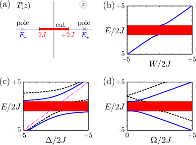
Figure 6: (a) The analytic properties of the $T$-matrix in the complex plane. The cut on the real axis is due to the propagation of (dressed) Bloch-waves. The two poles on the real axis correspond to two bound states and give rise to interference. (b-d) The spectrum $E_{n}$ of the Hamiltonian $H=H_{0}+V$ as a function of (a) the on-site-shift $W$ on the impurity for $\Omega=0$, (b) the detuning $\Delta$ for $\Omega/J=2$ and $W=0$ (solid lines), for $\Omega/J=4$ and $W=0$ (dashed lines), for $\Omega/J=2$ and $W/J=4$ (dash-dotted lines), (c) the Rabi-frequency $\Omega$ for $\Delta=W=0$ (solid lines), for $\Delta/J=4$ and $W=0$ (dashed lines), for $\Delta/J=W/J=4$ (dash-dotted lines). The continuous (scattering) spectrum, i.e. the Bloch-band $E_{k}$, is indicated as a shaded region $-2J<E_{k}<2J$, whereas the bound-state(s) $E_{B}$ are shown as (solid, dashed, dash-dotted) lines.

III.4 Discussion of Bound-states

For completeness we here derive the exact bound-state spectrum of $H$. For the exact scattering solution, detailed in Sec. III, the bound-states take the role of dressed states $|E_{\pm}\rangle$, which are responsible for the interference mechanism. We will show that for arbitrary $\Omega$ there are always two bound-states, provided $|\Delta-\Omega^{2}/W|>2J$. For $|\Delta-\Omega^{2}/W|\leq 2J$ one of the bound-states turns into a resonance, which makes the impurity completely transparent for the atom $A$, $T_{k}=1$. Furthermore, we will show that the bound-states for extends over several lattice sites for $\Omega,W,\Delta\sim J$. This is in marked contrast to the perturbative result, where the dressed states were localized on the impurity site, cf. Eq. (24a).

We obtain the bound states wavefunctions $|\phi_{B}\rangle$ from the homogeneous Lippmann-Schwinger equation

$$|\phi_{B}\rangle = G_{0}(E)V|\phi_{B}\rangle,$$ (29)

where $\phi_{B}$ denotes the bound-state with energy $E\equiv E_{B}$ ($|E_{B}|>2J$). Using the ansatz

$$|\phi_{B}\rangle = \sum_{j}\alpha_{j}|j\rangle+\beta|M\rangle$$ (30)

we find that the atomic and molecular amplitudes, $\alpha_{j}$ and $\beta$, satisfy

$$a_{j} = {\cal G}_{j}(E_{B})\left[W\alpha_{0}+\Omega\beta\right],$$ (31a)

$$\beta = {\cal G}_{M}(E_{B})\Omega\alpha_{0}.$$ (31b)

The atomic and molecular propagators are given by

$${\cal G}_{j}(E_{B}) = \langle j|G_{0}(E_{B})|0\rangle=\frac{e^{-|x_{j}|/r_{B}}\left[{\rm sign}\left(-E_{B}\right)\right]^{j}}{-2J\sinh\left(\kappa_{B}a\right)},$$

$${\cal G}_{M}(E_{B}) = \langle M|G_{0}(E_{B})|0\rangle=\frac{1}{E_{B}-\Delta},$$

and $r_{B}=a/{\rm acosh}(|E_{B}|/2J)>0$ denotes the size of the bound-state.

For convenience we first consider the case $\Omega=0$. There the molecular state decouples from the atomic ones, and we have one bound-state $|\phi_{1}\rangle=|M\rangle$ with energy $E_{1}=\Delta$. Moreover, for $W\neq 0$ we have another bound-state $|\phi_{2}\rangle$ with energy $E_{2}={\rm sign}(W)\sqrt{W^{2}+(2J)^{2}}$. Its amplitudes are given by $\beta=0$ and

$$\alpha_{j}=\left[{\rm tanh}\left(\frac{a}{r_{B}}\right)\right]^{1/2}e^{-|x_{j}|/r_{B}}\left[{\rm sign}(-W)\right]^{j},$$

with the size $r_{B}=a/{\rm arccos}\sqrt{1+(W/2J)^{2}}$. The spectrum of the system is plotted in Fig. 6(b) as a function $W$. For attractive (repulsive) interaction $W<0$ ($W>0$) the energy of the bound-state $\phi_{2}$, lies below (above) the Bloch-band, i.e. $E_{2}<-2J$ ($E_{2}>2J$), respectively. For $|W|<2J$ bound state $\phi_{2}$ extends over several lattice sites, while for $|W|\gg 2J$ it is localized on the impurity.

In the case $\Omega\neq 0$ a nontrivial solution of Eq. (31) requires

$$-E_{B}\left[1-\left(\frac{2J}{E_{B}}\right)^{2}\right]^{1/2} = W+\frac{\Omega^{2}}{E_{B}-\Delta},$$ (33)

which determines the bound-state spectrum $E_{B}(W,\Delta,\Omega)$. From Eq. (31) we obtain the atomic and molecular amplitudes as

$$\alpha_{j} = \beta\frac{E_{B}-\Delta}{\Omega}e^{-|x_{j}|/r_{B}}\left[{\rm sign}\left(-E_{B}\right)\right]^{j},$$ (34a)

$$\beta = \left[1+\frac{\left(E_{B}-\Delta\right)^{2}}{\Omega^{2}\sqrt{1-\frac{4J^{2}}{E_{B}^{2}}}}\right]^{-1/2}.$$ (34b)

We solve Eq. (33) by expressing one of the parameters, either $W$, $\Omega$ or $\Delta$, in terms of the bound-state energy $E_{B}$,

$$\Delta\left(E_{B}\right) = E_{B}+\frac{\Omega^{2}}{E_{B}\sqrt{1-4J^{2}/E_{B}^{2}}+W},$$ (35a)

$$\Omega\left(E_{B}\right) = \left[\left(\Delta-E_{B}\right)\left(E_{B}\sqrt{1-\frac{4J^{2}}{E_{B}^{2}}}+W\right)\right]^{1/2},$$ (35b)

$$W\left(E_{B}\right) = E_{B}\sqrt{1+\frac{4J^{2}}{E_{B}^{2}}}+\frac{\Omega^{2}}{E_{B}-\Delta}.$$ (35c)

Inverting the functions Eq. (35) for $E_{B}$ yields $E_{B}$ as a function of $\Delta$, $\Omega$ and $W$, respectively. For fixed $\Delta$, $\Omega$, $W$ we carry out the inversion by plotting in Fig. 6 the r.h.s. of Eq. (35)(a,b,c) as a function of $E_{B}$. In particular in Fig. 6(b) we plot detuning $\Delta$ as a function of $E_{B}$ for constant $\Omega$ and $W$, in Fig. 6(c) we plot Rabi-frequency $Omega$ as a function of $E_{B}$ for constant $\Delta$ and $W$, and in Fig. 6(d) we plot on-site shift $W$ as a function of $E_{B}$ for constant $\Delta$ and $\Omega$. In the following we will give a detailed discussion of Fig. 6.

For no background collisions, $W=0$, and arbitrary detuning $\Delta$, one always has two bound-states $\phi_{1,2}$ with energy $E_{1}<-2J$ and $E_{2}>2J$, respectively, see solid line in Fig. 6(c) corresponding to $\Omega=4J$. For $|\Delta|\gg\Omega$ the energy one bound-state approaches $\Delta$ and is wavefunction becomes localized on the impurity, while the energy the other approaches the Bloch-band and its wavefunction extends over several lattice-sites. For $\Delta=0$ the two bound-states are split symmetrically, and their energies are given by (see solid line in Fig. 6(d))

$$E_{1,2}=\pm\sqrt{2J^{2}+\sqrt{4J^{2}+\Omega^{2}}}.$$ (36)

The symmetric splitting allows for complete reflection at $E_{k}=0$. In the limit $\Omega\gg 2J$ we recover the perturbative result Eq. (24b), as the energies of the bound states approach $E_{\pm}=\pm\Omega$, with their wavefunctions given by the dressed states $|E_{\pm}\rangle$, cf. Eq. (24a).

For finite onsite shift, $W\neq 0$, we also have two bound-states provided $|\Delta_{\star}|\equiv|\Delta-\Omega^{2}/W|>2J$, see dashed lines in Fig. 6(c,d). With increasing detuning $\Delta$ the energy of the bound-state $\phi_{1}$ approaches the Bloch-band from below until crossing it for $-2J+\Omega^{2}/W<\Delta<+2J+\Omega^{2}/W$. In this parameter regime there is merely one bound state, while the other develops a resonance. This allows for perfect transparency at $E_{k}=\Delta-\Omega^{2}/W$.

Finally we remark that the size $r_{B}$ of the bound-states is inversely proportional to the separation of their energy $E_{B}$ from their Bloch-band. Thus for $|E_{B}|\ll 2J$ the wave-function of the bound-states extends over several lattice sites. For $|E_{B}|\gg 2J$ the bound-states are localized on the impurity and we recover the results of the previous section.

III.5 Wave-packet dynamics

As an illustration of the time-dependence of the interference mechanism we simulate the evolution of a gaussian wave-packet $\psi(t)$ with mean quasi-momentum $k=\pi/2a$ incident from the left of the impurity.

These wave-packets are obtained as superposition of the scattering solutions $\phi_{+}$ of Sec. III, i.e. their atomic and molecular amplitudes, $\alpha_{j}(t)=\langle j|\psi(t)\rangle$ and $\beta(t)=\langle M|\psi(t)\rangle$, are obtained as

$$\alpha_{j}(t) = \sum_{j^{\prime}}U_{j,j^{\prime}}(t)\alpha_{j^{\prime}}(0),$$ (37a)

$$\beta(t) = \sum_{j^{\prime}}U_{M,j^{\prime}}(t)\alpha_{j^{\prime}}(0),$$ (37b)

with the full propagator for the system given by

$$U_{j^{\prime},j}(t)=\sum_{B}\frac{e^{-(|x_{j^{\prime}}|+|x_{j}|)/r_{B}-iE_{B}t}{\rm sign}(-E_{B})^{j^{\prime}+j}}{\frac{|E_{B}|}{\sqrt{E_{B}^{2}+4J^{2}}}+\left[\frac{\Omega}{E_{B}-\Delta}\right]^{2}}+$$

$$+\frac{a}{2\pi}\int dke^{-iE_{k}t}\left[e^{+ik|x_{j^{\prime}}-x_{j}|}+r_{k}e^{+ik(|x_{j^{\prime}}|+|x_{j}|)}\right],$$

$$U_{M,j}(t)=\sum_{B}\frac{e^{-|x_{j}|/r_{B}-iE_{B}t}{\rm sign}(-E_{B})^{j}}{\sqrt{1+\frac{|E_{B}|(E_{B}-\Delta)^{2}}{\Omega^{2}\sqrt{E_{B}^{2}-4J^{2}}}}}+$$

$$+\frac{a}{2\pi}\int dke^{-iE_{k}t}\left[\frac{\Omega t_{k}}{E_{k}-\Delta+i0^{+}}e^{+ik(|x_{j}|)}\right].$$ (38)

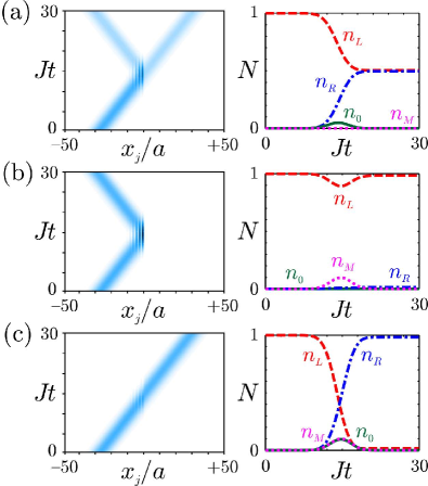
Figure 7: Evolution of a Gaussian wavepacket with mean quasi-momentum $k=\pi/2a$ for $W=2J$ and (a) $\Omega=0$, (b) $\Omega=2J$, $\Delta=0$, and (c) $\Omega=\Delta=2J$. On the left side the atomic density, $n(x_{j},t)$, of atoms $A$ is plotted (darker region correspond to higher density). The right side shows the corresponding population of atoms $A$ of the sites to the left, $n_{L}(t)$ (dashed-line), to the right, $n_{R}(t)$ (dashed-dotted line), and on the impurity site $n_{0}(t)$ (solid line), as well as the population of the molecular state, $n_{M}(t)$ (dotted line).

On the left side of Fig. 7 we plot the atomic populations of the individual sites, $n(x_{j},t)=|\alpha_{j}(t)|^{2}$. The right side shows the corresponding atomic populations of the atom $A$ on the left, $n_{L}=\sum_{j<0}n(x_{j},t)$ (dashed line), and on the right side of the impurity, $n_{R}=\sum_{j>0}n(x_{j},t)$ (dashed-dotted line). We also plot the population on the impurity, i.e. the atomic population, $n_{0}=n(x_{0},t)$ (solid line), and the molecular population, $n_{M}(t)=|\langle M|\psi(t)\rangle|^{2}$ (dotted line). The three different sets in Fig. 7 correspond to different coupling strengths, $\Omega$, and detunings, $\Delta$. For all cases we choose $W=2J$. In Fig. 7(a) we have $\Omega=0$: the atom is partially reflected from the impurity with $R_{k}=1$. In Fig. 7(b) we set $\Omega=2J$ and $\Delta=0$, which gives rise to complete reflection of the wavepacket, $R_{k}=1$. In Fig. 7(c) we have $\Omega=2J$, but now $\Delta=2J$. We have complete transmission of the atom through the impurity, $T_{k}=1$. All this is consistent with the results of Sec. III.

IV Many body scattering from an impurity

In this section we will analyze the evolution of a 1D lattice gas of many atoms $A$ interacting with an impurity atom $Q$. Since the statistics of the atoms $A$ plays a dominant role, we will consider the cases of fermionic and bosonic atoms, separately. In this context we will study analytically the limiting cases of an ideal Fermi-gas, an ideal Bose-gas and a Tonks-gas. An exact numerical treatment of the dynamics for the lattice-gas having arbitrary interaction $U$ is given in Ref. Daley .

IV.1 Ideal Fermi-gas

We first consider the case, where the probe atoms $A$ are spin-polarized fermions. The Hamiltonian for the system is given by

$$H = -J\sum_{j}\left(a_{j}^{{\dagger}}a_{j+1}+a_{j+1}^{{\dagger}}a_{j}\right)+\Delta|M\rangle\langle M|+$$ (39)

$$+\Omega\left(|M\rangle\langle Q|a_{0}+a_{0}^{\dagger}|Q\rangle\langle M|\right)+$$

$$+W_{Q}|Q\rangle\langle Q|a_{0}^{\dagger}a_{0}+W_{M}|M\rangle\langle{M}|a_{0}^{\dagger}a_{0},$$

where the operators $a_{j}^{\dagger}$ ($a_{j}$) create (annihilate) an atom $A$ on site $j$, and obey the canonical anti-commutation relations $\{a_{i},a_{j}^{\dagger}\}=\delta_{ij}$ and $\{a_{i},a_{j}\}=\{a_{i}^{\dagger},a_{j}^{\dagger}\}=0$. Moreover, $|Q\rangle$ ($|M\rangle$) denote the states with an atom $Q$ (a molecule in state $M$) on the impurity, and $W_{Q}$ ($W_{M}$) is the onsite-shift for an atom $A$ and an atom $Q$ (a molecule $M$) on the impurity.

For simplicity henceforth we will restrict ourselves to the case of equal on-site shifts $W_{M}=W_{Q}\equiv W$. In this case we may rewrite the Hamiltonian as

$$H = -J\sum_{j}\left(a_{j}^{{\dagger}}a_{j+1}+a_{j+1}^{{\dagger}}a_{j}\right)+Wa_{0}^{{\dagger}}a_{0}+$$ (40)

$$\Delta f^{\dagger}f+\Omega\left(f^{\dagger}a_{0}+a_{0}^{\dagger}f\right),$$

where the ladder operators $f^{\dagger}\equiv|M\rangle\langle Q|$ and $f\equiv|Q\rangle\langle M|$ obey standard fermionic anti-commutation relations and anti-commute with $a_{j}$ and $a_{j}^{\dagger}$. The corresponding equations of motions for $a_{j}$ and $f$ are linear, provided $W_{M}=W_{Q}$. Thus for a Fermi-gas of $N$ atoms $A$ the scattering off the impurity atom $Q$ will occur independently for each fermion $a_{k}$ with scattering amplitudes $t_{k}$ and $r_{k}$, according to their quasi-momentum $k$, cf. Eq. (17). The details of this calculation will be given below.

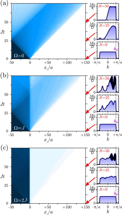
Figure 8: Evolution of a Fermi-gas with filling factor $\nu=1/2$ ($N=25$ particles on $M=50$ sites) after opening the switch at $t=0$. The effective Rabi-frequency is (a) $\Omega=0$, (b) $\Omega=J$ (c) $\Omega=2J$, and in all three cases we have $W=\Delta=0$. The left side shows the atomic density $n(x,t)$ (darker regions correspond to higher density), and the right side the momentum distribution $n(k,t)$ at time $t=0,M/2J,M/J$ (from bottom to top). The corresponding density distribution at this three times are indicated by arrow.

We will here detail the time-dependent scattering for a Fermi-gas of $N$ atoms $A$. For concreteness we assume the fermions to be initially trapped in a box of $M$ sites to the left the impurity atom $Q$. The corresponding wavefunction of the system is given by

$$|\Psi(t=0)\rangle=\prod_{n=1}^{N}\left[\sum_{j}\alpha_{j}(k_{n})a_{j}^{\dagger}\right]|Q\rangle,$$ (41)

$$\alpha_{j}(k_{n})=\sqrt{\frac{2}{M}}{\Big{\{}}\begin{array}[]{cc}\sin(k_{n}x_{j})&\mbox{for\enspace}-M{\leq}j\leq 1,\\ 0&\mbox{else},\end{array}$$ (44)

where the quasi-momenta $k_{n}=n\pi/(M+1)a$. This corresponds to a Fermi-sea filled up to $E_{F}=4J\sin^{2}(k_{F}a)$, where $k_{F}=\nu\pi/a$ is the Fermi-momentum and the initial filling-factor $\nu=N/(M+1)$.
At time $t=0$ we open the impurity (cf. Fig. 1(b)), and from Eq. (40) we obtain the evolution of the system as

$$|\Psi(t)\rangle=\prod_{n=1}^{N}\left[\sum_{j}\alpha_{j}(k_{n},t)a_{j}^{\dagger}+\beta(k_{n},t)f^{\dagger}\right]|Q\rangle,$$ (45a)

$$\alpha_{j}(k_{n},t)=\sum_{j^{\prime}}U_{j,j^{\prime}}(t)\alpha_{j^{\prime}}(k_{n}),$$ (45b)

$$\beta(k_{n},t)=\sum_{j^{\prime}}U_{M,j^{\prime}}(t)\alpha_{j^{\prime}}(k_{n}),$$ (45c)

where $U_{\alpha,j}(t)$ are the single-particle propagators, cf. Eq. (38). According to Eq. (45a) the scattering from the impurity occurs independently for each particle in the initial Fermi sea, with scattering amplitudes $t_{k}$ and $r_{k}$ given in Eq. (17) for $0<k\leq k_{F}$. The atomic and molecular densities are thus given by the sum of the probabilities for the single fermions in the Fermi-gas,

$$n(x_{j},t) = \langle a_{j}^{\dagger}a_{j}\rangle_{t}=\sum_{n=1}^{N}|\alpha_{j}(k_{n},t)|^{2},$$ (46a)

$$n_{M}(t) = 1-n_{Q}(t)=\sum_{n=1}^{N}|\beta(k_{n},t)|^{2}.$$ (46b)

Moreover, after opening the switch the atomic quasi-momentum distribution in the Fermi-gas for the semi-infinite system is given by

$$n(k,t) = \frac{a}{2\pi}\sum_{j,j^{\prime}}e^{-ik(x_{j^{\prime}}-x_{j})}\langle a_{j^{\prime}}^{\dagger}a_{j}^{\phantom{{\dagger}}}\rangle_{t}$$ (47)

$$= \frac{a}{2\pi}\sum_{n=1}^{N}\Big{|}\sum_{j}e^{-ikx_{j}}\alpha_{j}(k_{n},t)\Big{|}^{2}.$$

In Fig. 8(a,b,c) we show the evolution for a Fermi-sea with $\nu\approx 3/4$, i.e. $N=38$ particles initially on $M=50$ sites. For each simulation we have $W=\Delta=0$, but the driving varies as $\Omega/J=0,1,2$ in Fig. 8(a,b,c) respectively. On the left side we plot the atomic density $n(x_{j},t)$ (darker regions correspond to higher density). To the right we plot the respective momentum profiles $n(k,t)$ for the Fermi-gas at times $t=0,M/2J,M/J$ (from bottom to top). This times are indicated by arrows each figure.

In Fig. 8(a) we see the evolution of the noninteracting system, $\Omega=0$. The atomic cloud expands freely to the right after opening the switch at $t=0$. The corresponding momentum distribution is initially given by $n(k,t=0)\approx\theta(k_{F}-|k|)Ma/2\pi$ (see profile at the bottom). With progressing time $0<t<M/2J$ the gas develops a forward peak at $k=\pi/2a$ (see profile in the middle) until becoming asymmetric as $n(k,t=M/J)\approx(M/2\pi)\theta(k_{F}-k)2\theta(k)$ for $t\leq M/J$ (see profile at the top).

In Fig. 8(b) we show the behavior for for weak laser driving, $\Omega=J$. We notice that there is already substantial blocking by the impurity. The corresponding momentum profiles show that the blocking is mainly due to the complete reflection of fermions with quasi-momentum near $k=\pi/2a$ to $k^{\prime}=-\pi/2a$.

In Fig. 8(c) we plot the densities for resonant driving with $\Omega=2J$. The transport through the impurity is efficiently blocked by the impurity atom, as the initial densities $n(x_{j},t=0)$ and $n(k,t=0)$ are almost completely preserved.

In the following we will consider the number of particles on the right side of the impurity,

$$N_{R}(t) = \sum_{j>0}n(x_{j},t),$$ (48)

and the corresponding particle current through the impurity, $I_{R}$.

$$I_{R}(t) = \frac{dN_{R}}{dt}(t).$$ (49)

They characterize the behavior of the switch.

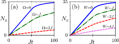
Figure 9: The number of atoms $A$ transmitted through the impurity as a function of time $t$, $N_{R}(t)$, for a Fermi-gas with $\nu=1$. (a) We gave $\Delta=W=0$ and the coupling is $\Omega=0$ (solid line), $\Omega=J$ (dashed-dotted line), $\Omega=2J$ (dashed line). In (b) there is no coupling, $\Omega=0$, but the background interaction are $W=0,J,2J,4J$ (solid, dash-dotted, dashed, dotted line). The system establishes a constant particle current up to $t\approx 50/J$ $\Delta=W=0$ and the coupling is $\Omega=0$ (solid line), $\Omega=M/J=50/J$, and saturates until all $N=50$ atoms $A$ passed the impurity.

In Fig. 9(a) we show the number of particles $N_{R}(t)$, for the same parameters as in Fig. 8, i.e. for each the initial filling factor $\nu\approx 3/4$ and $W=\Delta=0$. The solid line shows $N_{R}$ for the no coupling to the impurity, $\Omega=0$, and corresponds to the densities shown in Fig. 8(a). The dashed-dotted line shows the behavior for $\Omega=J$, cf. Fig.8(b), and the dashed line corresponds to $\Omega=2J$, i.e. Fig.8(c). Moreover, in Fig. 9(b) we show the number of particles $N_{R}(t)$, for initial filling factor $\nu\approx 3/4$ and $\Omega=\Delta=0$, but for an onsite shift $W=0,J,2J,4J$ (see solid, dash-dotted, dashed, dotted line), respectively. In general, after a short transient period, of the order of the inverse tunneling rate $1/J$, the number of particles on the right side of the impurity increases linearly with $t$. Thereby the system establishes a roughly constant flux of particles $I_{R}$ through the impurity. The flux persists up to $t\approx M/J$, which is indicated by a vertical dotted line in Fig. 9(a,b). Then the population on the left side of the impurity is substantially depleted and therefore $N_{R}(t)$ saturates until all particles tunneled through the impurity, yielding $N_{R}(t)=N$ and $I_{R}(t)=0$ for $t\rightarrow\infty$.

We are interested in the linear regime. From Eq. (46a) we obtain the constant average current as (cf. the Landauer-formula)

$$I_{R}=\frac{dN_{R}}{dt}=\frac{1}{2\pi}\int_{0}^{k_{F}}dkv_{k}T_{k},$$ (50)

where $v_{k}=-2Ja\sin(ka)$ is the group-velocity of the quasi-particles with quasimomentum $k$, $k_{F}=\nu\pi/a=N\pi/(M+1)a$ the Fermi-quasimomentum and $T_{k}$ the corresponding transmission coefficients, cf. Eq. (17). Thus the average current is obtained by integrating the Fano-profiles $T_{k}=1-R_{k}$, see e.g. Fig 5, up to the Fermi-momentum.

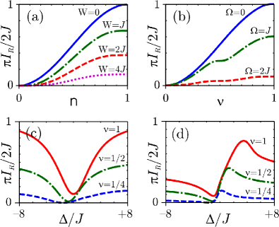
Figure 10: The quasi-steady state atomic current $I_{R}$ through the impurity. Its dependence on the filling factor $\nu$ is shown in (a) for $\Omega=0$ but $W=0,J,2J,4J$, and in (b) for $W=\Delta=0$ but $\Omega=0,J,2J$. The dependence of $I_{R}$ on the detuning $\Delta$ is shown in (c) for $\Omega=2J$, $W=0$ and in (d) for $\Omega=W=2J$.

For an uncoupled impurity, $W=\Omega=0$, we have $T_{k}=1$. Thus the current is given up to a constant by the Fermi-energy,

$$I_{R}^{(0)} = \frac{E_{F}}{2\pi}=\frac{2J}{\pi}\sin^{2}\left(\frac{\nu\pi}{2}\right).$$ (51)

In Fig. 8(b) we plot the dependence of $I_{R}^{(0)}$ as a function of the filling factor $\nu$ as a solid line.

For a finite on-site shift, $|W|>0$, but no laser-driving, $\Omega=0$, we have $T_{k}<1$, see Eq. (19) and Fig. 5(a). Thus the current through the switch decreases as

$$I_{R}^{(W)} = \frac{E_{F}}{2\pi}-\frac{W^{2}}{2\pi E_{0}}{\rm arccoth}\left(\frac{W^{2}+2JE_{F}}{E_{0}E_{F}}\right)$$ (52)

where $E_{0}=\sqrt{W^{2}+4J^{2}}$ is the modulus of the bound-state energy. The exponential decay of $I_{R}^{(W)}$ with increasing coupling strength $W$, i.e. the arccoth-term in Eq. (52), is characteristic for a system with one bound-state. The dependence of the current $I_{R}^{(W)}$ on the filling-factor $\nu$ is shown in Fig. 10(a). The solid line shows the non-interacting value, $W=0$, while the dash-dotted, dashed, dotted line correspond to $W=J,2J,4J$, respectively.

However, for resonant driving at $\Omega>0$ and couplings $W=\Delta=0$ we obtain a symmetric Fano-profile for $R_{k}$ with respect to $k=\pi/2a$, see Fig. 5(b). Therefore, by integrating the latter profiles we obtain the current as

$$I_{R}^{(\Omega)} = \frac{E_{F}}{2\pi}-\frac{E_{+}E_{-}^{2}}{2\pi\left(E_{+}^{2}-E_{-}^{2}\right)}{\rm arccoth}\left(\frac{E_{-}^{2}+2JE_{F}}{E_{+}E_{F}}\right)+$$ (53)

$$-\frac{E_{+}^{2}E_{-}}{2\pi\left(E_{+}^{2}-E_{-}^{2}\right)}{\rm arccot}\left(\frac{E_{+}^{2}+2JE_{F}}{E_{-}E_{F}}\right),$$

with $E_{\pm}=\sqrt{\sqrt{\Omega^{4}+4J^{4}}\pm 2J^{2}}$. The arccoth-term in Eq. (53) gives the mean effect of the reflection as that typical of a system with one bound-state, while the oscillating arccot-term is induced by the presence of two interfering poles in the scattering matrix. The current Eq. (53) is plotted in Fig. 10(b) as a function of the initial filling factor $\nu$ for the uncoupled impurity, $\Omega=0$ (solid line), for $\Omega=J$ (dashed-dotted line), and for $\Omega=2J$ (dashed line). For finite driving the current $I_{R}^{(\Omega)}$ shows a plateau at $\nu=1/2$, as all the Bloch-waves near $k=\pi/2a$ are completely reflected from the impurity (see Fig. 5(b)). From Eq. (53) we obtain that already for $\Omega\sim 4J$ the current of particles through the impurity is completely suppressed for arbitrary filling $\nu$, i.e. up to Fermi-energy $E_{F}=4J$.

In the following we discuss the dependence of the current for $\Omega>0$ on the detuning $\Delta$. In Fig. 10(c) we show the current $I_{R}$ for $\Omega=2J$ but still $W=0$ as a function of the detuning $\Delta$ for several initial densities $\nu$. The solid line corresponds to commensurate initial filling, $\nu=1$, the dash-dotted line to half-filling, $\nu=1/2$, and the dotted line to a dilute Fermi-gas with $\nu=1/4$. The current shows a symmetric profile with a minimum at $\Delta\approx-2J\cos^{3}(\nu\pi/2)$ and approaches its threshold value $I_{R}^{(0)}$ for $|\Delta|\gg\Omega$. Notice that the resonance for the many-body Fermi-gas with increasing density from the bottom of the Bloch-band, $\Delta\approx-2J$, toward the middle of the band, $\Delta=0$.

For finite $W=2J$ (see Fig. 10(d)) the dependence shows an asymmetric profile and reaches its threshold value $I_{R}^{(W)}$ (cf. Eq. (52)) for large detuning, $|\Delta|\gg\Omega^{2}/|W|$. We notice that although the single fermions in the Fermi-sea scatter independently, we obtain a finite current for $\Omega<J$, even on resonance. This is caused by the fact that the various fermionic modes $a_{k}$ see the resonance a different (energy-dependent) detuning $\Delta-E_{k}$, which leads to a shift of the minimum (and maximum) of the transmitted current proportional to the density of the Fermi-gas, see Fig. 10(c,d). However, in the limit of strong driving $\Omega\gg J$ we recover the features of perfect blocking for $\Delta\approx 0$ and of perfect transmission for $\Delta\approx\Omega^{2}/W$.

IV.2 Ideal Bose-gas

We now consider the case, where the probe atoms $A$ are spin-less non-interacting bosons. The Hamiltonian for the system is given by

$$H = -J\sum_{j}\left(a_{j}^{\dagger}a_{j+1}+{\rm h.c.}\right)+\Delta|M\rangle\langle M|+$$ (54)

$$+W_{Q}|Q\rangle\langle Q|a_{0}^{\dagger}a_{0}+W_{M}|M\rangle\langle M|a_{0}^{\dagger}a_{0}+$$

$$+\Omega\left(|M\rangle\langle Q|a_{0}+a_{0}^{\dagger}|Q\rangle\langle M|\right),$$

where the operators $a_{j}^{\dagger}$ ($a_{j}$) create (annihilate) an atom $A$ on site $j$, and obey the canonical commutation relations $[a_{i},a_{j}^{\dagger}]=\delta_{ij}$ and $[a_{i},a_{j}]=[a_{i}^{\dagger},a_{j}^{\dagger}]=0$. Moreover, $|Q\rangle$ ($|M\rangle$) denote the states with an atom $Q$ (a molecule in state $M$) on the impurity, and $W_{Q}$ ($W_{M}$) is the onsite-shift for an atom $A$ and an atom $Q$ (a molecule $M$) on the impurity. As in the previous section we will henceforth restrict ourselves to the case of equal on-site shifts $W_{M}=W_{Q}\equiv W$. In this case we may rewrite the Hamiltonian as

$$H = -J\sum_{j}\left(a_{j}^{\dagger}a_{j+1}+a_{j+1}^{\dagger}a_{j}\right)+Wa_{0}^{\dagger}a_{0}+$$ (55)

$$+\Delta\sigma^{+}\sigma^{-}+\Omega\left(\sigma^{+}a_{0}+a_{0}^{\dagger}\sigma^{-}\right),$$

where the pauli operators $\sigma^{+}\equiv|M\rangle\langle Q|$ and $\sigma^{-}\equiv|Q\rangle\langle M|$ obey canonical anti-commutation relations and commute with $a_{j}$ and $a_{j}^{\dagger}$. The Hamiltonian (55) corresponds a multi-mode Jaynes-Cummings model.

In the following we will consider the scattering of a gaussian wavepacket of $N$ bosons $A$, all initially occupying the same single particle state, $\alpha(x_{j},t=0)$, approaching the impurity atom $Q$ with mean quasi-momentum $\pi/a>k_{0}>0$ and width ${\delta k}_{0}\ll\pi/a$. The corresponding wavefunction for the system is given by

$$|\Psi(t=0)\rangle = |Q\rangle\frac{1}{\sqrt{N!}}\left[\sum_{j}\alpha(x_{j},t=0)a_{j}^{\dagger}\right]^{N}|{\rm vac}\rangle,$$ (56)

$$\alpha_{0}(x_{j},0) = {\cal N}e^{-{\delta k}_{0}^{2}(x_{j}-x(0))+ik_{0}x_{j}},$$ (57)

where for $\delta k_{0}\ll\pi/a$ the normalization is given by ${\cal N}^{2}=(2\delta k_{0}^{2}a^{2}/\pi)^{1/2}=n_{0}/N$ in terms of the peak density of the gaussian wavepacket, $n_{0}\equiv n(x(0),t=0)$, and $x(0)\ll 0$ denotes the mean position of the particles $A$ at $t=0$.

For $\Omega=0$ the equations of motion for $a_{j}$ decouple from $\sigma^{-}$. Therefore, we obtain the scattering of the bosons $A$ by the impurity, as

$$|\Psi(t)\rangle = |Q\rangle\frac{1}{\sqrt{N!}}\left[\sum_{j}\alpha(x_{j},t)a_{j}^{\dagger}\right]^{N}|{\rm vac},$$ (58)

where the single-particle wavefunction for finite $W$ was already obtained in Sec. III. For this case all the results obtained in Sec. III hold, and we obtain e.g. the density as $N$ times the single particle result, $n(x_{j},t)=N|\alpha(x_{j},t)|^{2}|$.

IV.2.1 Linearization of the impurity

For $\Omega\gg J\gg|\Delta|,|W|$, we obtained in Sec. III that the population of the molecular state was strongly suppressed, i.e. as $(J/\Omega)^{2}$, and thus we approximate $\sigma^{z}\rightarrow-1$. Thus we linearize the spin, i.e. set $\sigma^{+}\rightarrow b^{\dagger}$ and $\sigma^{-}\rightarrow b$, where $b$ and $b^{\dagger}$ obey canonical commutation relations. The scattering of the bosons $A$ by the impurity is given by

$$|\Psi(t)\rangle \approx \frac{1}{\sqrt{N!}}\left[\sum_{j}\alpha_{j}(t)a_{j}^{\dagger}+\beta(t)b^{\dagger}\right]^{N}|{\rm vac}\rangle_{A},$$ (59)

where the single-particle wavefunction $\alpha_{j}(t)$ and the amplitude $\beta(t)$ of the molecular state $b^{\dagger}|{\rm vac}\rangle\equiv\sigma^{+}|Q\rangle=|M\rangle$, were obtained in Sec. III (see Eq. (38)).

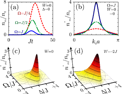
Figure 11: Scattering of a Gaussian wavepacket of bosonic atoms $B$ with mean quasi-momentum $k_{0}$ and width ${\delta k}_{0}$ as obtained by linearizing the impurity (see text). (a) Molecular population as a function of time for a narrow wavepacket with $k=\pi/a$ and $\delta k_{0}=\pi/100a$ for $\Omega=J,J/2,J/4$ (solid, dash-dotted, dashed line). (a) The maximal attained molecular population , $n_{m}^{\star}$, during the interaction process with a weakly coupled impurity ($\Omega=J$, $\Delta=W=0$), as a function of the quasi-momentum $k_{0}$ of the incoming wavepacket. The three lines correspond a wavepacket with width $\delta k_{0}=\pi/200a,\pi/50a,\pi/20a$ (solid, dash-dotted and dashed line). The dependence of $n_{m}^{\star}$ on the parameters $\Omega$ and $\Delta$ for $k=\pi/2a$ and $\delta k_{0}=\pi/50a$ in (c) without the presence of background collisions, $W=0$, and in (d) for an onsite-shift $W=2J$.

Self-consistency of the replacement $\sigma_{z}\rightarrow-1$ requires that the obtained molecular population $n_{m}(t)\ll 1$. From the linearization we obtain the molecular population as (see App. A)

$$n_{m}(t) = \frac{n_{0}}{4{\delta k}_{0}^{2}\pi}\left|\int dk\frac{\Omega t_{k}e^{-iE_{k}t}}{E_{k}-\Delta}e^{-\tilde{k}^{2}/4{\delta k}_{0}^{2}-i\tilde{k}x(0)}\right|^{2},$$ (60)

where $\tilde{k}\equiv k-k_{0}$, and the Fourier-integral is obtained analytically e.g. by using a saddle-point method, see App. A. We find that the maximal attained molecular population, $n_{m}^{\star}$, is proportional to the initial density $n_{0}$ of the gas. In the case of a broad resonance, $\Omega>\delta k_{0}$, we find

$$n_{m}^{*} \approx \frac{n_{0}\Omega^{2}v_{0}^{2}/a^{2}}{\left(E_{0}-\Delta\right)^{2}v_{0}^{2}/a^{2}+\left[\Omega^{2}+W\left(E_{0}-\Delta\right)^{2}\right]^{2}},$$ (61)

with $E_{0}=-2J\cos(k_{0}a)$ and $v_{0}=2J\sin(k_{0}a)$. Moreover, for a extremely narrow resonance, $\Omega<\delta k_{0}$ and $|\Delta|<J$, one obtains

$$n_{m}^{*} \approx \frac{n_{0}}{2\delta k_{0}^{2}a}\frac{\Omega^{2}}{W^{2}+v_{\star}^{2}/a^{2}}e^{-\left(k_{0}-k_{\star}\right)^{2}/2\delta k_{0}^{2}},$$ (62)

where $v_{\star}=2J\sin(k_{\star}a)$ and $k_{\star}\approx\arccos(-\Delta/2J)$ denotes the position of the maximum of $T_{k}/(E_{k}-\Delta)^{2}$.

In Fig. 11(a) we show the molecular population, $n_{m}$, as obtained by the replacement $\sigma_{z}\rightarrow-1$. In Fig. 11(a) we plot the $n_{m}(t)/n_{0}$ for an incoming gaussian wavepacket with $k_{0}=\pi/2a$ and $\delta k_{0}=0.01\pi/a$ for driving $\Omega=J/4$ (dashed line), $\Omega=J/2$ (dashed-dotted line) and $\Omega=J$ (solid line). In all three cases we have $\Delta=W=0$. We see that with increasing Rabi-frequency $\Omega$ the attained molecular-population quickly drop as $\sim J^{2}/\Omega^{2}$, and that the molecular-population closely resembles the density distribution $n(x_{j},t=0)$ of the atomic-cloud $A$. In Fig. 11(b) we plot the maximal attained population, $n_{m}^{*}$, as a function of the incoming momentum of the gas, $k_{0}$, for $\Omega=J$ and $W=\Delta=0$. The four lines correspond to different width $\delta k_{0}$ of the wavepacket, i.e. $\delta k_{0}=0.001\pi/a$ (solid line), $\delta k_{0}=0.01\pi/a$ (dashed line), $\delta k_{0}=0.1\pi/a$ (dash-dotted line) and $\delta k_{0}=0.2\pi/a$ (dashed line). For a given width $\delta k_{0}$ the molecular population attains its maximum for $k_{0}=\pi/2a$, i.e. where we have complete reflection of the wave-packet (see Fig. 5(b)). At the point of complete-reflection, $k_{0}=\pi/2a$ the population attains its overall maximum for a narrow momentum-distribution, i.e. for $\delta k_{0}\rightarrow 0$ we have $n_{m}\approx 4n_{0}$ for $\Omega=J$ and $\Delta=W=0$. The dependence of $n_{m}^{\star}$ on the detuning $\Delta$ and the Rabi-frequency $\Omega$ is shown in Fig. 11(c,d) for $W=0$ and $W=-2J$, respectively. In both figures the gaussian wavepacket has $k_{0}=\pi/2a$ and $\delta k_{0}=0.02\pi/a$, i.e. initially extends about $\sim\pi/a\delta k_{0}=50$ lattice sites. For $W=0$ we have complete reflection of the wavepacket for $\Delta=0$, and the attained molecular population is maximal, $n_{m}\approx 3n_{0}$, for $\Omega\approx 2J$ and $\Delta\approx 0$ (see Fig. 11(c)). However, for finite $W=-2J$ we have also complete transmission of the wavepacket, i.e. for $\Delta=\Omega/W$. From Fig. 11(d) we notice that for a given $Omega$ the maximal population is shifted from $\Delta\approx 0$ towards the point, where one has complete transmission of the wavepacket, i.e. $\Delta\approx\Omega/W$. However, the overall maximum of $n_{m}^{\star}$ in both cases, $W=0$ and $W=-2J$, is attained for $\Omega\approx 2J$ and for stronger driving quickly drops as $n_{m}^{\star}\approx n_{0}(2J/\Omega)^{2}$. As the replacement $\sigma^{-}\rightarrow b$ is self-consistent for a dilute gas with densities $n_{0}\ll(n_{m}^{\star}/n_{0})^{-1}$, we see from 11 that the approximation holds, even on resonance $\Delta=0$, for strong driving $\Omega>4J$ up to densities as high as $n_{0}\sim 5$ and for small densities $n_{0}<1$ only fails for $\Delta\approx 0$ and $\Omega\approx 2J$.

IV.2.2 Time-dependent Variational Ansatz

In the following we use a time-dependent variational Ansatz to describe the behavior of the many-body wavefunction in near resonance $\Delta\approx 0$ for $\Omega\sim J$, i.e. in the regime where the approximation $\sigma_{z}\rightarrow-1$ fails already for small densities, $n_{0}>0.05$. As a generalization of Eq. (30) for $N\geq 1$ bosonic atoms $A$ we choose as an number-conserving Ansatz for the state of the system

$$|\Psi(t)\rangle = c_{Q}(t)|Q\rangle\frac{\left[a_{Q}(t)^{\dagger}\right]^{N}}{\sqrt{N!}}|{\rm vac}\rangle+$$ (63)

$$c_{M}(t)|M\rangle\frac{\left[a_{M}(t)^{\dagger}\right]^{N-1}}{\sqrt{({N-1})!}}|{\rm vac}\rangle,$$

where $a_{\sigma}(t)=\sum_{j}\alpha_{j,\sigma}(t)a_{j}^{\dagger}$ represent two non-orthogonal time-dependent modes for the field of the bosonic atoms $A$ given that the impurity is in state $\sigma=Q,M$, and the amplitudes for the impurity, $c_{\sigma}(t)$, and for the bosonic wavepackets, $\alpha_{j,\sigma}(t)$, are normalized as $\sum_{\sigma}|c_{\sigma}(t)|^{2}=\sum_{j}|\alpha_{j,\sigma}(t)|^{2}$. The equation of motion for variational parameters, $c_{\sigma}(t)$ and $\alpha_{j,\sigma}(t)$, are obtained by minimizing the corresponding action (cf. App. B)

$$S(t) = \frac{\langle\dot{\Psi}_{t}|\Psi_{t}\rangle-\langle\Psi_{t}|\dot{\Psi}_{t}\rangle}{2i}-\langle\Psi_{t}|H|\Psi_{t}\rangle$$ (64)

with respect to $c_{\sigma}(t)^{*}$ and $\alpha_{j,\sigma}(t)^{*}$, as a set of coupled non-linear differential equations, which we integrate numerically. Thus we obtain the dynamics of the system.

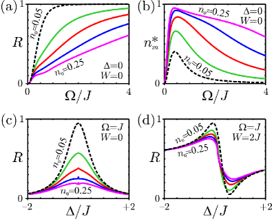
Figure 12: Evolution of a Gaussian wavepacket with mean quasi-momentum $k=\pi/2a$ and width $\delta k_{0}=0.02\pi/a$ obtained from the variational Ansatz Eq. (63). In (a) the reflection coefficient $R$ is plotted as a function of the Rabi-frequency $\Omega$ for $\Delta=W=0$, and (b) shows the corresponding attained maximal molecular population $n_{m}^{\star}$ during the interaction with the impurity atom. The reflection coefficient as a function of the detuning $\Delta$ for $\Omega=J$ and (c) $W=0$ and (d) $W=2J$. The various solid lines correspond to initial densities $n_{0}=0.1,0.15,0.20,0.25$. The dotted-line is for $n=0.05$ and corresponds to a linearization of the impurity, see Eq. (59).

In Fig. 12 we show the obtained reflection-coefficient

$$R=\lim_{t\rightarrow\infty}\frac{1}{N}\sum_{j<0}n(x_{j},t)$$ (65)

and the attained peak molecular population $n_{m}^{\star}$ for a Gaussian-wavepacket with narrow momentum $k_{0}=\pi/2a$, i.e. $\delta k_{0}=0.02\pi/a\ll\pi/a$ for initial density $n_{0}=0.05,0.1,0.15,0.20,0.25$ (values indicated in plots). In Fig. 12(a) (Fig. 12(b)) we plot $R$ ($n_{m}^{\star}$) as a function of the Rabi frequency $\Omega$ for $\Delta=W=0$, i.e. when complete reflection of the wavepacket was predicted by the bosononic approximation of the spin. The reflection shows a non-linear behavior in the density for $\Omega>.1$, i.e. decreases as $\sim 1/n_{0}$ with increasing density $n_{0}$. While for $n_{0}=0.05$ (see dotted line) we have complete reflection of the wavepacket for $\Omega>2J$, for higher densities we still have a finite transmission at $\Omega=2J$. From Fig. 12(a) we see that with increasing density the transmission coefficient rapidly deviates from the low(zero)-density result and approaches a linear behavior in $\Omega$ already for $n_{0}=1/4$. In Fig. 12(a) we plot the dependence of $n_{m}^{\star}$ on $\Omega$, which shows that the maximal population is attained for $\Omega\approx J/2$ and decreases as $\sim(J/\Omega)^{2}$ for $\Omega\gg Jn_{0}$. Moreover, we see that with increasing density, $n_{0}>0.10$, the peak in the molecular population, $n_{m}^{\star}$, is no longer linear in the density as was predicted by linearization, cf. Eq. (61) and cf. Eq. (61), but saturates toward the unitary limit $n_{m}^{\star}\approx 1$. The dependence of the reflection coefficient $R$ on the detuning $\Delta$ is plotted in Fig. 12(c) for $\Omega=J$ and $W=0$ and in Fig. 12(c) for $\Omega=J$ and $W=2J$. In the limit of a very dilute Bose-gas (see dashed lines for $n_{0}=0.05$) we obtain the single-particle result $T=|t(k_{0})|^{2}$ given by Eq. (17), showing a symmetric Fano-profile for $W=0$ and an asymmetric Fano-profile for $W=2J$, (see also Fig. 5(b,d)). We notice that at such weak-driving as $\Omega=J$ the peak (and the asymmetry) in the Fano-profiles are suppressed with increasing density. However, for strong driving $\Omega\gg 4Jn_{0}$ we recover the features of complete reflection (complete transmission) through the impurity site as was already predicted by the linearization of the impurity.

IV.3 Hard-core Bosons

We now consider the limit of a strongly interacting Bose-gas. Its Hamiltonian is given by

$$H = -J\sum_{j}\left(a_{j+1}^{\dagger}a_{j}+{\rm h.c.}\right)+\frac{U}{2}\sum_{j}a_{j}^{\dagger}a_{j}^{\dagger}a_{j}a_{j}+$$ (66)

$$+\Delta|M\rangle\langle M|+\Omega\left(|M\rangle\langle Q|a_{0}+a_{0}^{\dagger}|Q\rangle\langle M|\right)+$$

$$+W_{Q}a_{0}^{\dagger}|Q\rangle\langle Q|a_{0}+W_{M}a_{0}^{\dagger}a_{0}|M\rangle\langle M|$$

where the onsite-shift for two-bosons $A$ on the same site, $U$, by far exceeds the tunneling rate $J$, i.e. $U{\gg}J$. Since double occupation of a site by two atoms $A$ is strongly suppressed, we may eliminate those excitation from $H$, e.g. by imposing $a_{j}^{2}\equiv 0$. In the following we will focus on the limiting case $U/J\rightarrow\infty$, i.e. that of a Tonks gas. In this limit we may fermionize the Hamiltonian (66) via a Jordan-Wigner transformation (JWT) Sachdev , which maps the commuting fields for the hard-core bosons, $a_{j}$, and the pseudo-spin of the impurity, $\sigma^{-}\equiv|M\rangle\langle Q|$, onto anticommuting fields, $c_{j}$ and $f$, respectively. The JWT is given by

$$a_{j}=c_{j}\prod_{l<j}\left(1-2c_{l}^{\dagger}c_{l}\right),a_{j}^{\dagger}=c_{j}^{\dagger}\prod_{l<j}\left(1-2c_{l}^{\dagger}c_{l}\right),$$ (67a)

$$\sigma^{-}=f\prod_{l}\left(1-2c_{l}^{\dagger}c_{l}\right),\sigma^{+}=f^{\dagger}\prod_{l}\left(1-2c_{l}^{\dagger}c_{l}\right).$$ (67b)

The fields $c_{j}$ and $f$ describe fermionic excitations for the new joint vacuum state of the system, $|{\rm vac}\rangle_{CF}\equiv|Q\rangle|{\rm vac}\rangle$. We rewrite the Hamiltonian (66) in terms of the fermionic excitations, $c_{j}$ and $f$, and obtain

$$H = -J\sum_{j<M}\left(c_{j+1}^{\dagger}c_{j}+{\rm h.c.}\right)+$$ (68)

$$+\Delta f^{\dagger}f+\Omega\left(-1\right)^{\hat{N}_{R}}\left(f^{\dagger}c_{0}+{\rm h.c.}\right)+$$

$$+W_{Q}ff^{\dagger}c_{0}^{\dagger}c_{0}+W_{M}f^{\dagger}fc_{0}^{\dagger}c_{0},$$

where $\hat{N}_{R}=\sum_{j>0}c_{j}^{\dagger}c_{j}=\sum_{j>0}a_{j}^{\dagger}a_{j}$ is the number of particles to the right of the impurity site. The Hamiltonian for the fermionic excitations, $c_{j}$ and $f$, is the same as the one obtained for the Fermi-gas, cf. Eq. (40), except for the appearance of the phase-factor $(-1)^{\hat{N}_{R}}$ for the coupling $\Omega$ to the impurity.

We proceed by detailing the time-dependent scattering of a tonks gas with $N$ atoms $A$ off the impurity atom $Q$. We assume that at time $t=0$ the atoms $A$ are trapped within a box of $M$ sites to the left on impurity site. This corresponds to a fermi-sea of the fermionic modes $c_{j}$, and the state of the system at $t=0$ is given by (see also Sec.IV.1)

$$|\Psi(0)\rangle=\prod_{n=1}^{N}\left[\sqrt{\frac{2}{M}}\sum_{j<0}\sin\left(k_{n}x_{j}\right)c_{j}^{\dagger}\right]|{\rm vac}\rangle_{CF}$$

$$=|Q\rangle\sum_{{\bf j}<0}(-1)^{S({\bf j})}\prod_{n=1}^{N}\left[\sqrt{\frac{2}{M}}\sin\left(k_{n}x_{j_{n}}\right)a_{j_{n}}^{\dagger}\right]|{\rm vac}\rangle_{A},$$ (69)

where $k_{n}=n\pi/(M+1)a$ are the quasi-momenta of the fermionic excitations, ${\bf j}=(j_{1},j_{2},\ldots,j_{N})$ (with $j_{p}\neq j_{q}$) denotes the position of the $N$ bosons and $(-1)^{S({\bf j})}$ the permutational sign of ${\bf j}$, i.e. $S({\bf j})=\sum_{j_{p}>j_{q}}1$. Due to the cumbersomeness of the many-body wavefunction in terms of the bosonic operators $a_{j}$, it is preferable to deal within the fermionic picture and extract the quantities of interest from the correlations for the fermions. The density $n(x_{j},t)$ of the hardcore bosons $A$ corresponds to the density for the fermions $c$, while the correlations, $\rho(x_{i},x_{j},t)$, and the momentum distribution of the Tonks gas, $n(k,t)$, differ from those of a Fermi-gas, as

$$n(x_{j},t) = \langle a_{j}^{\dagger}a_{j}\rangle=\langle c_{j}^{\dagger}c_{j}\rangle,$$ (70a)

$$\rho(x_{i},x_{j},t) = \langle a_{i}^{\dagger}a_{j}\rangle=\langle c_{i}^{\dagger}\prod_{l=i}^{j}\left[1-2c_{l}^{{\dagger}}c_{l}\right]c_{j}\rangle,$$ (70b)

$$n(k,t) = \frac{a}{2\pi}\sum_{m,n}e^{-ik\left(x_{m}-x_{n}\right)}\langle a_{m}^{\dagger}a_{n}\rangle$$

$$= \frac{a}{2\pi}\sum_{m,n}e^{-ik\left(x_{m}-x_{n}\right)}\langle c_{m}^{\dagger}\prod_{l=m}^{n}\left[1-2c_{l}^{\dagger}c_{l}\right]c_{n}\rangle.$$

Diagonalizing the single-particle density matrix $\rho(x_{i},x_{j},t)$ one obtain the condensate fraction $N_{0}(t)$ as the largest eigenvalue and the wavefunction of the quasi-condensate $\psi_{0}(x_{j},t)$ as the corresponding eigenmode. In the following we denote density of the quasi-condensate as $n_{0}(x_{j},t)$ and its momentum distribution as $n_{0}(k,t)$.

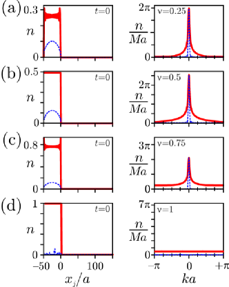
Figure 13: Initial density distribution of a gas of hard core bosons. The gas is trapped on $M=50$ to the left of the impurity site, $x_{j}=0$, and the fillings factor is (a) $\nu=1/4$, (b) $\nu=1/2$, (c) $\nu=3/4$ and (d) $\nu=1$, respectively. Shown are the atomic density $n$ (solid line) and the mode of the quasi-condensate $n_{0}$ (dotted line), in position (left column) and momentum space (right column).

In Fig. 13 we plot the initial density for a Tonks-gas trapped on $M=50$ sites for various filling factors $\nu=1/4,1/2,3/4,1$, i.e. we have $N=13,25,38,50$ particles for Fig. 13(a,b,c,d), respectively. The solid lines in the plot on the left shows the density in position space, $n(x_{j})$, and the dotted lines show the contribution of the largest eigenmode of the single-particle-density matrix $\rho(x_{i},x_{j})$, $n_{0}(x_{j})$. To the right we plot the corresponding quasi-momentum distributions of the gas, $n(k)$ (solid line), and for the largest eigenmode of $\rho(x_{i},x_{j})$, $n_{0}(k)$ (dotted line). While the density merely resembles that of a homogeneous Fermi-gas with local filling factor $\nu$, the momentum distributions strongly differs from the typical Fermi-sea (cf. Fig. 8) as it shows a sharp peak at $k=0$, as one would expect from a condensate. However, the condensed fraction $N_{0}\equiv\sum_{j}n_{0}(x_{j})$ (see dashed lines within the same figures) is not macroscopic, as it amounts only to $\approx\sqrt{N}$ particles in the gas and thus the behavior of the Tonks-gas significantly differs from that of a true BEC. In fact we notice that the momentum distribution shows considerable wings, which account for the depletion in the quasi-condensate. Moreover, with increasing density $\nu$ the number of particle in the quasi-condensate depletes considerably until vanishing completely for $\nu=1$ (see Fig. 13(d)), where the system attains a Mott-insulator with no phase-correlations.

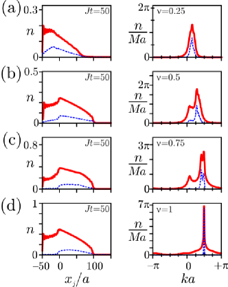
Figure 14: Free evolution of a gas of hard core bosons. The gas was initially trapped on $M=50$ to the left of the impurity site, $x_{j}=0$, and the fillings factor is (a) $\nu=1/4$, (b) $\nu=1/2$, (c) $\nu=3/4$ and (d) $\nu=1$, respectively. Shown are the atomic density $n$ (solid line) and the density of the quasi-condensate $n_{0}$ (dotted line), in position (left column) and momentum space (right column) at a time $t=M/J$ after opening the mirror.

We now detail the free ($\Omega=W_{Q}=0$) evolution of the Tonks gas after having opened the switch at $t=0$. From Eq. (68) we obtain the state of the system at time $t$ to be given by (cf. Sec.IV.1)

$$|\Psi_{t}\rangle = |Q\rangle\prod_{n=1}^{N}\left[\alpha_{j}(k_{n},t)c_{j}^{\dagger}\right]|{\rm vac}\rangle,$$ (71a)

$$\alpha_{j}(k_{n},t) = \sqrt{\frac{2}{M}}\sum_{j^{\prime}<0}U_{j,j^{\prime}}(t)\sin(k_{n}x_{j}),$$ (71b)

where $U_{j,j^{\prime}}(t)$ denotes the free single-particle propagator, cf. Eq. (38) with $W=\Omega=0$. The density $n(x_{j},t)$ of the hardcore-bosons $A$ corresponds to that of the fermions, given by Eq. (46a). In Fig. 14 we show to the left the densities $n(x,t)$ of the Tonks-gas (solid lines) and of the condensate mode $n_{0}(x_{j},t)$ (dashed line) at time $t=M/J=50/J$ after opening the switch. To the right we plot the corresponding momentum distributions, $n(k,t)$ and $n_{0}(k,t)$. As in Fig. 13 the subplots Fig. 14(a,b,c,d) correspond to an initial filling factor $\nu=1/4,1/2,3/4,1$, respectively. The density of the Tonks-gas, $n(x_{j},t)$, corresponds to the one obtained for a Fermi-gas (see e.g. Fig. 8(a) for $\nu=1/2$), and shows the spreading of the gas through the impurity. The corresponding momentum distribution of the Tonks-gas, $n(k,t)$, is shifted away from $k=0$ towards $k>0$ and spread in momentum space, due to the tunneling of the particles through the impurity site. Moreover, after a brief transient period starts developing an new additional peak at $k\approx k_{F}/2=\nu\pi/2$, which gains in magnitude until reaching its maximum value at $t=M/J$. This corresponds to the dynamical formation of a quasi-condensate $n_{0}(k,t)$ Rigol , which now propagates as a wave-packet through the impurity with $k\approx\nu\pi/2$ (see dotted lines in Fig. 14). The number of particle is the quasi-condensate, $N_{0}(t)=\sum_{j}n_{0}(x_{j},t)$, gives the magnitude of the peak and grows with progressing time until it saturates at $t\approx M/J$. At this time the Tonks gas on the right side of the impurity is significantly depleted and one has $N_{0}(t)\approx\sqrt{N}$. The dynamical formation of a quasi-condensate propagating with $k>0$ is clearly seen for filling factors $\nu>1/2$, where it momentum peak at $k=k_{F}/2$ exceeds the magnitude of the initial $k=0$ coherent fraction. For the Mott-insulating state (commensurate filling $\nu=1$) the situation is particularly clear: the mott-insulator melts through the impurity (see left side of Fig. 14(d)) and forms a quasi-condensate propagating as a coherent wavepacket with velocity $v_{k}=2Ja$ through the lattice. Thereby the initially flat develops a sharp peak at $k=\pi/a$ (see right side of Fig. 14(d)). The number of particles in the quasi-condensate increases until reaching $\sim\sqrt{N}$ for $t=M/J$. It saturates as the initial Mott-insulating state is significantly depleted. Moreover, from the evolution of the density distributions in position space (see plots on the right of Fig. 14(a-d)) we see that, although the quasi-condensate only amounts to a fraction of atoms in the system, its profile $n_{0}(x_{j},t)$ describes the transmitted part of the Tonks-gas through the impurity accurately, i.e. up to a multiplicative factor.

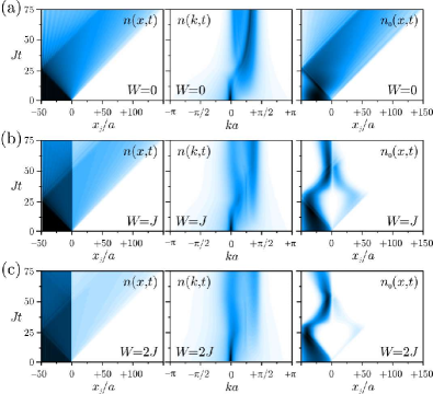
Figure 15: Evolution of a gas of hard-core bosons with filling factor $\nu=1/2$ for $\Omega=0$ and (a) $W=0$, (b) $W=J$, (c) $W=2J$. Shown are the density $n(x_{j},t)$ (left column), the momentum distribution $n(k,t)$ and the density of the quasi-condensate $n_{0}(x_{j},t)$.

In the presence of a finite on-site shift, $W_{Q}\neq 0$, but with driving $\Omega=0$, the Hamiltonian is still bilinear in the fermionic modes $c_{i}^{\dagger}$ and $c_{j}$. The evolution of the system is given by Eq. (71), but now with $U_{j^{\prime},j}(t)$ being the single-particle propagator for $W\neq 0$. In Fig. 15(a,b,c) we show the evolution of a Tonks gas with $\nu=1/2$ for $W=0$, $W=J$ and $W=2J$, respectively. On the left side we plot the density distribution, $n(x_{j},t)$, in the middle the momentum distribution, $n(k,t)$, and to the right the quasi-condensate $n_{0}(x_{j},t)$. Darker regions correspond to regions of higher density. For no interaction, $W=0$, the particles freely tunnel through the impurity. The momentum distribution is shifted towards $k>0$ as well as being broadened. At $t\approx M/2J=25/M$ an additional peak in the momentum distribution is formed at $k\approx\pi/3a$, which corresponds to the mode of the quasi-condensate, $n_{0}(x_{j},t)$, tunneling through the impurity (see Fig. 15(a)). For $W=J$ the tunneling of particles through the impurity site is partially blocked and the dynamical formation of a monochromatic mode with $k>0$ is suppressed, as is see from the. Thereby the condensate mode $n_{0}(x_{j},t)$ remains mainly localize to the left side of the impurity. For $W=2J$ we see that only a small fraction of atoms passes through the impurity and the momentum distribution remains centered at $k=0$, although becoming slighty broader. We also see that the condensed fraction of atoms in the condensate is efficiently hindered from passing the impurity and remains localized to the left of the impurity site.

In the presence of a finite coupling $\Omega>0$, the Hamiltonian is no more bilinear in $c_{j}^{\dagger}$ and $c_{j}$, due the appearance of the nonlinear factor $(-1)^{\hat{N}_{R}}=\prod_{j>0}(1-2c_{j}^{\dagger}c_{j})$, which makes a description of the time-dependent scattering in terms of the fermionic modes $c_{j}$ in the general case as difficult as integrating out the full many-body Schrödinger equation (66) for the hard-core bosons $A$. However, the contribution of the nonlinear factor $(-1)^{\hat{N}_{R}}$ to the dynamics is negligible for strong driving, $\Omega\gg J,|\Delta|,W$, and also for low densities, $\nu\ll 1$. In this case the number of atoms on the right $N_{R}(t)\ll 1$, and those we set $\hat{N}_{R}\rightarrow 0$ in Eq. (68). The state of the system is given by

$$|\Psi_{t}\rangle = \prod_{n=1}^{N}\left[\alpha_{j}(k_{n},t)c_{j}^{\dagger}+\beta(k_{n},t)f^{\dagger}\right]|{\rm vac}\rangle,$$ (72a)

$$\alpha_{i}(k_{n},t) = \sqrt{\frac{2}{M}}\sum_{j<0}U_{i,j}(t)\sin(k_{n}x_{j}),$$ (72b)

$$\beta(k_{n},t) = \sqrt{\frac{2}{M}}\sum_{j<0}U_{M,j}(t)\sin(k_{n}x_{j}),$$ (72c)

where $U_{\alpha,j}(t)$ denotes the full single-particle propagator, cf. Eq. (38). In this regime the density distribution of the Tonks-gas, $n(x_{j},t)$, corresponds to that of a Fermi-gas (see e.g. the left side in Fig. 8).

For the general case of many bosons $A$, arbitrary coupling strengths, and even finite $U$, we refer to the exact numerical simulation given in Ref. Daley . These simulations allow to test the behavior of the gas for essentially arbitrary repulsion $U$ and density $\nu$, i.e. for the full crossover regime from a weakly interacting dilute Bose-gas up to a dense Tonks gas.

V Conclusion

We have studied a scheme utilizing quantum interference to control the transport of atoms in a 1D optical lattice by a single impurity atom. The two internal state represent a qubit (spin-1/2), which in one spin state is perfectly transparent to the lattice gas, and in the other spin state acts as a single atom mirror, confining the lattice gas. This allows to “amplify” the state of the qubit, and provides a single-shot quantum non-demolition measurement of the state of the qubit. We have derived exact analytical expression for the scattering of a single atom by the impurity, and gave approximate expressions for the dynamics a gas of many interacting bosonic of fermionic atoms.

A numerical study of this dynamics based on time-dependent DMRG techniques, which complements the present discussion, will be presented in Ref. Daley .

Appendix A Scattering of Gaussian Wavepackets

We consider the dynamics of a bosonic $N$-particle state of the form

$$|\Psi_{t}\rangle = \frac{1}{\sqrt{N!}}\left[\sum_{j}\alpha_{t}(x_{j})a_{j}^{\dagger}+\beta_{t}b^{\dagger}\right]^{N}|{\rm vac}\rangle,$$

where at $t=0$ the gaussian wave-packet is given by $\beta_{0}=0$ and

$$\alpha_{0}(x_{j}) = {\cal N}_{0}e^{-{\delta k}_{0}^{2}\left(x_{j}-x_{0}\right)+ik_{0}x_{j}},$$

where $x_{0}\ll 0$ ($k_{0}>0$) is the mean position (momentum) and ${\delta k}_{0}<\pi/a$ the width in momentum space at $t=0$. For ${\delta k}_{0}\ll\pi/a$ we may take the continuum limit $\sum_{j}\rightarrow\int dx/a$ and obtain ${\cal N}_{0}\approx\left(2{\delta k}_{0}^{2}a^{2}/\pi\right)^{1/4}$, and ${\delta x}_{0}\approx 1/2{\delta k}_{0}\gg a/\pi$. The momentum representation of the is given by

$$\tilde{\alpha}_{0}(k) = \left(a/2\pi\right)^{1/2}\sum_{j}e^{-i*k*x_{j}}\alpha_{0}(x_{j})$$

$$\approx \left(2\pi{\delta k}_{0}^{2}\right)^{-1/4}e^{-\left(k-k_{0}\right)^{2}/4{\delta k}_{0}^{2}-i\left(k-k_{0}\right)x_{0}}.$$

A.1 Molecular density

For the evolution we are interested at the population of the molecular state, which follows as

$$n_{m}(t) = \langle b^{\dagger}b\rangle_{t}=N\left|\sum_{j}U_{M,j}(t)\alpha_{0}(x_{j})\right|^{2}$$

$$= N{\cal N}_{0}^{2}\left|\sum_{j}U_{M,j}(t)e^{-{\delta k}_{0}^{2}\left(x_{j}-x_{0}\right)+ik_{0}x_{j}}\right|^{2},$$

where $U_{M,j}(t)=\langle M|e^{-iHt}|j\rangle$ is the single particle propagator. We introduce the peak of the initial atomic density $n_{0}\equiv n(x_{0},t=0)=N{\cal N}_{0}^{2}\approx N\left(2/\pi\right)^{1/2}{\delta k}_{0}a$.

For the scattering off the particles, i.e. for $|x_{0}|\gg r_{B}$, we may neglect the finite range of the bound-state and have

$$n_{m}(t) \approx N\left|\sum_{j}\frac{a}{2\pi}\int dke^{-iE_{k}t}\frac{\Omega t_{k}}{E_{k}-\Delta}e^{ik|x_{j}|}\alpha_{0}(x_{j})\right|^{2}$$

$$= N\left(\frac{a}{2\pi}\right)\left|\int dke^{-iE_{k}t}\frac{\Omega t_{k}}{E_{k}-\Delta}\tilde{\alpha}_{0}(k)\right|^{2}.$$

Thus we have

$$n_{m}(t) = n_{0}\left|f_{t}\right|^{2},$$

$$f_{t} = \frac{1}{2{\delta k}_{0}\sqrt{\pi}}\int dk\frac{\Omega t_{k}}{E_{k}-\Delta}e^{-iE_{k}t-\left(\frac{k-k_{0}}{2{\delta k}_{0}}\right)^{2}-i\left(k-k_{0}\right)x_{0}}.$$

For the Fourier transform we use a saddle-point method, however, we have to distinguish which one is narrower, either the width of the wave-packet, $\delta k_{0}$, or the width of dressing profile.

A.2 Broad Fano-profile

For a broad resonance, i.e. $\Omega t_{k}/(E_{k}-\Delta)$ slowly varying on the Bloch band we expand the integral around $k\approx k_{0}$, i.e. with

$$E_{k}\approx E_{0}+v_{0}\left(k-k_{0}\right)+\frac{1}{2m_{0}}\left(k-k_{0}\right)^{2},$$

$$\frac{\Omega t_{k}}{E_{k}-\Delta}\approx\frac{\Omega t_{0}}{E_{0}-\Delta},$$

where energy $E_{0}\equiv E_{k}\mid_{k=k_{0}}$, velocity $v_{0}\equiv\partial E_{k}/\partial k\mid_{k=k_{0}}$ and effective mass $m_{0}\equiv 1/(\partial^{2}E_{k}/\partial^{2}k)\mid_{k=k_{0}}$. Notice that $m_{k}=-1/a^{2}E_{k}$ for the explicit shape of the Bloch-band and choice of the origin in the band-middle.

Thereby we obtain

$$n_{m}(t) = n_{0}\frac{\delta k_{t}}{\delta k_{0}}e^{-2\delta k_{t}x_{t}^{2}}{\cal D}_{0},$$

where the linear propagation, spreading and the dressing are

$$x_{t} = x_{0}+v_{0}t,$$

$$\delta k_{t} = \frac{\delta k_{0}}{\sqrt{1+\left(2\delta k_{0}^{2}a^{2}E_{0}t\right)^{2}}},$$

$${\cal D}_{0} = \frac{\Omega^{2}|t_{k}|^{2}}{\left(E_{k}-\Delta\right)^{2}}\mid_{k=k_{0}}$$

$$= \frac{\Omega^{2}}{\left(E_{0}-\Delta\right)^{2}+\left[\Omega^{2}+W\left(E_{0}-\Delta\right)\right]^{2}a^{2}/v_{0}^{2}}.$$

We notice that at $t_{\star}=-x_{0}/v_{0}=|x_{0}/v_{0}|$ we attain a maximal molecular density of

$$n_{m}(t_{\star}) = n_{0}\frac{{\cal D}_{0}}{\sqrt{1+\left(2\delta k_{0}^{2}a^{2}E_{0}t\right)^{2}}}.$$

For $E_{0}\approx 0$ we might neglect the broadening/spreading. We recognize that ${\cal D_{0}}$ is maximal for such detuning $\Delta$ and initial momentum $k_{0}$ where

$$E_{\star} \approx \Delta-W\frac{\Omega^{2}}{W^{2}+v_{\star}^{2}/a^{2}},$$

is on the bloch-band. This corresponds to the position of the Fano-profile. As $v_{\star}^{2}/a^{2}=4J^{2}-E_{\star}^{2}$ the Equation for $E_{\star}$ is implicitly cubic gives the same recursive equation. Thus the maximal density for a broad resonance $\Omega\gg|J-\Delta|$ is suppressed as

$$n_{m}(t_{\star})\approx n_{0}\frac{v_{0}^{2}/a^{2}}{\Omega^{2}},$$ (73)

while far off resonance $|\Delta|\gg\Omega$ we have

$$n_{m}(t_{\star})\approx n_{0}\frac{(\Omega/\Delta)^{2}}{1+(aW/v_{0})^{2}}.$$ (74)

A.3 Narrow Fano-profile

In the second case, that of a narrow resonance, i.e. a sharp Fano profile, we have that the dressing factor is narrower than the Gaussian wavepacket, hence we approximate via a Saddle-point method. We expand the dressing function,

$${\cal D}_{k}=\frac{\Omega t_{k}}{E_{k}-\Delta}=\left[\frac{ia\Omega}{v_{k}}+\frac{E_{k}-\Delta}{\Omega}\left(1+\frac{iaW}{v_{k}}\right)\right]^{-1},$$

around the momentum $k_{\star}$ where $|{\cal D}_{k}|$ is maximal,

$${\cal D}_{k}\approx C_{0}e^{+iC_{1}(k-k\star)a-\frac{1}{2}C_{2}(k-k_{\star})^{2}a^{2}},$$ (75)

with

$$C_{0} = \frac{-i\Omega}{\zeta},$$

$$C_{1} = \frac{\gamma_{\star}+iW}{\zeta}-\frac{im_{\star}}{\gamma_{\star}}\left(1+i\frac{E_{\star}-\Delta}{\zeta}\right),$$

$$C_{2} = \left(\frac{\gamma_{\star}+iW}{\zeta}\right)^{2}-\frac{im_{\star}}{\gamma_{\star}}\left(\frac{\gamma+iW}{\zeta}+\frac{2\Omega^{2}}{\zeta^{2}}\right)$$

$$+\frac{m_{\star}^{2}}{\gamma_{\star}^{2}}\left[1+\frac{\left(E_{\star}-\Delta\right)^{2}}{\zeta^{2}}\right],$$

$$\zeta \equiv \frac{\Omega^{2}+\left(E_{\star}-\Delta\right)\left(W-i\gamma_{\star}\right)}{\gamma_{\star}},$$

where $E_{\star}=E(k_{\star})$, $\gamma_{\star}=\partial E(k)/\partial ka\mid_{k=k_{\star}}=v(k_{\star})/a$, $m_{\star}=\partial^{2}E(k)/\partial(ka)^{2}=-E(k_{\star})$ are the lowest expansion coefficient of the dispersion relation $E(k)=-2J\cos(ka)$ at $k=k_{\star}$.

The position of its maximum $k_{\star}$ is obtained from the expansion (75)by requiring $\Im[C_{1}]=0$ with

$$\Im[C_{1}]=\gamma_{\star}\frac{\Omega^{2}W+\left(E_{\star}-\Delta\right)\left(\gamma_{\star}^{2}+W^{2}\right)}{\Omega^{4}+2\left(E_{\star}-\Delta\right)\Omega^{2}W+\left(E_{\star}-\Delta\right)\left(\gamma_{\star}^{2}+W^{2}\right)}$$

$$-\frac{m_{\star}}{\gamma_{\star}}\frac{\left[\Omega^{2}+\left(E_{\star}-\Delta\right)W\right]^{2}}{\Omega^{4}+2\left(E_{\star}-\Delta\right)\Omega^{2}W+\left(E_{\star}-\Delta\right)\left(\gamma_{\star}^{2}+W^{2}\right)}.$$

In the limit of interest (i.e. near the middle of the Bloch-band), we have $|m_{k}/\gamma_{k}|=|\cot(ka)|\ll 1$ thus we obtain the energy of the maximum as a series

$$E_{\star}\approx\Delta-\frac{W\Omega^{2}}{\gamma_{\star}^{2}+W^{2}}+\frac{m_{\star}\gamma_{\star}^{2}\Omega^{4}}{\left(\gamma_{\star}^{2}+W^{2}\right)^{3}}+{\cal O}^{2}\left(m_{\star}\right).$$ (76)

Since $\gamma_{\star}$, $m_{\star}=-E_{\star}$ all depend on $k_{\star}$ the series gives implicitly the value of $k_{\star}$. Moreover, we notice that the truncation to first order in $m_{\star}$ yields the exact result for $W=0$.

Then with

$$\zeta \approx \frac{\Omega^{2}}{\gamma_{\star}-iW}\left[1-i\frac{m_{\star}}{\gamma_{\star}}\left(\frac{\Omega\gamma_{\star}}{W^{2}+\gamma_{\star}^{2}}\right)^{2}\right],$$

$$C_{0} \approx \frac{-\left(W+i\gamma_{\star}\right)/\Omega}{1-im_{\star}\gamma_{\star}\Omega^{2}/\left(\gamma_{\star}^{2}+W^{2}\right)^{2}},$$

$$C_{1} \approx \frac{\gamma_{\star}^{2}+W^{2}}{\Omega^{2}}-\frac{m_{\star}W}{\gamma_{\star}^{2}+W^{2}},$$ (77)

$$C_{2} \approx \left(\frac{\gamma_{\star}^{2}+W^{2}}{\Omega^{2}}\right)^{2}-i\frac{m_{\star}}{\gamma_{\star}}\frac{\gamma_{\star}^{2}-W^{2}-4i\gamma_{\star}W}{\Omega^{2}},$$

we can compute the Fourier-integral and obtain

$$|f_{t}|^{2} = |C_{0}|^{2}|A(t)|e^{-\frac{1}{2}\Re\left[A(t)\left(2\delta k_{0}x(t)+i\frac{k_{0}-k_{\star}}{\delta k_{0}}\right)^{2}+\left(\frac{k_{0}-k_{\star}}{\delta k_{0}}\right)^{2}\right]},$$

$$A(t) = \left[1+2\delta k_{0}^{2}a^{2}\left(C_{2}+im_{\star}t\right)\right]^{-1},$$ (78)

$$x(t) = x_{0}+v_{\star}t-aC_{1}.$$

For $E_{\star}\approx 0$, i.e. near the middle of the Bloch-band, we might neglect the spreading of the wave-packet, i.e. $m_{\star}\approx 0$. Then we have

$$|C_{0}|^{2} = C_{1}=\frac{W^{2}+v_{\star}^{2}/a^{2}}{\Omega^{2}}=\sqrt{C_{2}},$$

$$|f(t)|^{2} = \frac{C_{1}\exp\left[-\frac{2\delta k_{0}^{2}x(t)^{2}+C_{1}^{2}\left(k_{0}-k_{\star}\right)^{2}a^{2}}{1+2\delta k_{0}^{2}a^{2}C_{1}^{2}}\right]}{1+2{\delta k_{0}}^{2}a^{2}C_{1}^{2}}.$$ (80)

In the limit $\Omega\rightarrow 0^{+}$ the probability $|f(t)|^{2}$ vanishes as

$${\rm max}_{t}|f(t)|^{2} \approx \frac{\Omega^{2}}{W^{2}+v_{\star}^{2}/a^{2}}\frac{\exp\left[-\frac{\left(k_{0}-k_{\star}\right)^{2}}{2\delta k_{0}^{2}}\right]}{2{\delta k_{0}}^{2}a^{2}}.$$ (81)

Appendix B Variational Ansatz

For the Ansatz (63) we obtain the action (64) as

$$\begin{gathered}S=\frac{1}{2}\sum_{\sigma}\Big{[}c_{\sigma}^{*}\frac{\partial c_{\sigma}}{\partial t}-\Delta\delta_{\sigma M}|c_{\sigma}|^{2}+N_{\sigma}|c_{\sigma}|^{2}\sum_{j}\alpha_{j,\sigma}\\ \times\left(i\frac{\partial\alpha_{j,\sigma}}{\partial t}+J\alpha_{j+1,\sigma}+J\alpha_{j-1,\sigma}-W\delta_{j0}\alpha_{j,\sigma}\right)\Big{]}\\ -\Omega\sqrt{N}c_{M}^{*}c_{Q}\left(\sum_{j}\alpha_{j,M}^{*}\alpha_{j,Q}\right)^{N}\alpha_{j,Q}+{\rm c.c.},\end{gathered}$$

with $c_{\sigma}\equiv c_{\sigma}(t)$, $\alpha_{j,\sigma}\equiv\alpha_{j,\sigma}(t)$ and $N_{Q}=N_{M}+1=N$.

Minimizing the action $S$ with respect to $c_{\sigma}^{*}$ and $\alpha_{j,\sigma}$, we obtain after some algebra,

$$ic_{M}^{*}\frac{\partial c_{M}}{\partial t} = \Delta|c_{M}|^{2}+\lambda-(N-1)\frac{\lambda+\lambda^{*}}{2},$$

$$ic_{Q}^{*}\frac{\partial c_{Q}}{\partial t} = \lambda^{*}-N\frac{\lambda+\lambda^{*}}{2},$$

$$i|c_{M}|^{2}\frac{\partial\alpha_{j,M}}{\partial t} = |c_{M}|^{2}\left(-J\sum_{\pm}\alpha_{j\pm 1,M}+W\delta_{j0}\alpha_{j,M}\right)$$

$$-\frac{\lambda-\lambda^{*}}{2}\alpha_{j,M}+\frac{\lambda}{s}\alpha_{j,Q},$$

$$i|c_{Q}|^{2}\frac{\partial\alpha_{j,Q}}{\partial t} = |c_{Q}|^{2}\left(-J\sum_{\pm}\alpha_{j\pm 1,Q}+W\delta_{j0}\alpha_{j,Q}\right)$$

$$+\frac{\lambda-\lambda^{*}}{2}\alpha_{j,Q}+\frac{N-1}{N}\frac{\lambda^{*}}{s^{*}}\alpha_{j,M}+\frac{\lambda^{*}\delta_{j0}}{N\alpha_{0,Q}^{*}}$$

where the overlap $s$ and the effective coupling $\lambda$ are given by

$$s = \sum_{j}\alpha_{j,M}^{*}\alpha_{j,Q},$$

$$\lambda = \Omega\sqrt{N}c_{M}^{*}c_{Q}s^{N-1}\alpha_{0,Q}.$$

References

- (1) C. Cohen-Tannoudji, J. Dupont-Roc, and G. Grynberg, Atom-Photon Interactions : Basic Processes and Applications, (Wiley Science Paperback Series, New York, 1992).
- (2) J. McKeever, A. Boca, A. D. Boozer, R. Miller, J. R. Buck, A. Kuzmich and H. J. Kimble, Science 303, 1992 (2004).
- (3) G. Nogues, A. Rauschenbeutel, S. Osnaghi, M. Brune, J. M. Raimond, and S. Haroche, Nature (London) 400, 239 (1999).
- (4) P. Maunz, T. Puppe, I. Schuster, N. Syassen, P. W. H. Pinkse, and G. Rempe, Nature (London) 428, 50 (2004).
- (5) S. Rinner, H. Walther, and E. Werner, Phys. Rev. Lett. 93, 160407 (2004)
- (6) For a review see e.g. D. Jaksch and P. Zoller, Annals of Physics 315, 52-79 (2005).
- (7) M. Greiner, O. Mandel, T. Esslinger, T. W. Hänsch, and I. Bloch, Nature (London) 415, 39 (2002).
- (8) O. Mandel, M. Greiner, A. Widera, T. Rom, T. W. Hänsch, and I. Bloch, Phys. Rev. Lett. 91, 010407 (2003).
- (9) T. Stöferle, H. Moritz, C. Schori, M. Köhl, and T. Esslinger, Phys. Rev. Lett. 92, 130403 (2004).
- (10) E. L. Bolda, E. Tiesinga, and P. S. Julienne, Phys. Rev. A 66, 013403 (2002).
- (11) R. Ciurylo, E. Tiesinga, and P. S. Julienne, Phys. Rev. A 71, 030701(R) (2005)
- (12) M. Holland, J. Park, and R. Walser, Phys. Rev. Lett. 86, 1915 (2001).
- (13) M. Theis, G. Thalhammer, K. Winkler, M. Hellwig, G. Ruff, R. Grimm, and J. H. Denschlag, Phys. Rev. Lett. 93, 123001 (2004).
- (14) A. Recati, P. O. Fedichev, W. Zwerger, J. von Delft, and P. Zoller, Phys. Rev. Lett. 94, 040404 (2005).
- (15) R. B. Diener, B. Wu, M. G. Raizen, and Q. Niu, Phys. Rev. Lett. 89, 070401 (2002).
- (16) V. B. Braginsky and F. Y. Khalili, Quantum Measurement, (Cambridge University Press, UK, 1992).
- (17) See, for example, G. Johansson, P. Delsing, K. Bladh, D. Gunnarsson, T. Duty, A. Käck, G. Wendin, and A. Aassime, Proceedings of NATO ARW ”Quantum Noise in Mesoscopic Physics”, (Delft, June 2002); cond-mat/0210163.
- (18) A. Micheli, A. J. Daley, D. Jaksch, and P. Zoller, Phys. Rev. Lett. 93, 140408 (2004).
- (19) D. Jaksch, C. Bruder, J. I. Cirac, C. W. Gardiner, and P. Zoller, Phys. Rev. Lett. 81, 3108 (1998).
- (20) S. Datta, Electronic Transport in Mesoscopic Systems, (Cambridge University Press, UK, 1997).
- (21) G. D. Mahan, Many Particle Physics, (Plenum US, Third edition, 2000).
- (22) L. S. Levitov, in Quantum Noise in Mesoscopic Physics, Ed. Y. V. Nazarov (Kluwer Academic Publishers, 2002).
- (23) M. A. Cazalilla and J. B. Marston, Phys. Rev. Lett. 88, 256403 (2002), and references cited therein.
- (24) A. J. Daley et al., in preparation.
- (25) M. Lukin, Rev. Mod. Phys. 75, 457 (2003).
- (26) See, for example, S. Sachdev, Quantum Phase Transitions, (Cambridge University Press, UK, 1999).
- (27) M. Rigol and A. Muramatsu, Phys. Rev. Lett.93, 230404 (2004).